Gaining Insight With Recursive Partitioning Of Generalized Linear Models

ePub

WU

Institutional Repository

Thomas Rusch and Achim Zeileis

Gaining Insight With Recursive Partitioning Of Generalized Linear Models

Working Paper

Original Citation:

Rusch, Thomas and Zeileis, Achim (2011) Gaining Insight With Recursive Partitioning Of

Generalized Linear Models. Research Report Series / Department of Statistics and Mathematics,

109. WU Vienna University of Economics and Business, Vienna.

This version is available at: http://epub.wu.ac.at/3143/

Available in ePubWU_{: June 2011}

ePubWU_{, the institutional repository of the WU Vienna University of Economics and Business, is}

provided by the University Library and the IT-Services. The aim is to enable open access to the scholarly output of the WU.

Gaining Insight With

Recursive Partitioning Of

Generalized Linear Models

Thomas Rusch, Achim Zeileis

Research Report Series

Institute for Statistics and Mathematics

Gaining Insight With Recursive Partitioning Of

Generalized Linear Models

Thomas Rusch

Achim Zeileis

01.01.2011

Recursive partitioning algorithms separate a feature space into a set of disjoint rectangles. Then, usually, a constant in every partition is fitted. While this is a simple and intuitive approach, it may still lack interpretability as to how a specific relationship between dependent and independent variables may look. Or it may be that a certain model is assumed or of interest and there is a number of candidate variables that may non-linearily give rise to different model parameter values. We present an approach that combines generalized linear models with recursive partitioning that offers enhanced interpretability of classical trees as well as providing an explorative way to assess a candidate variable’s influence on a parametric model. This method conducts recursive partitioning of a generalized linear model by (1) fitting the model to the data set, (2) testing for parameter instability over a set of partitioning variables, (3) splitting the data set with respect to the variable associated with the highest instability. The outcome is a tree where each terminal node is associated with a generalized linear model. We will show the methods versatility and suitability to gain additional insight into the relationship of dependent and independent variables by two examples, modelling voting behaviour and a failure model for debt amortization.

Keywords: model-based recursive partitioning; generalized linear models; functional trees; parameter instability; maximum likelihood

1 Introduction

In many fields, classic parametric models are still dominant in statistical modelling and often rightly so. They demand some insight into the data generating process as well a a strong theoretical foundation to be applicable and as such force a researcher to be clear about the question she wants answered and to put a great deal of thought into collecting data and setting up the statistical model. They have the undeniable advantage to be interpretable in light of the research questions. They usually pose restrictions on the relationship between the explanatory variables and the target variables. A very common restriction is to define the

∗

Institute for Statistics and Mathematics, WU (Vienna University of Economics and Business), Austria

†

functional relationship between (transformations of) the independent and (transformations of) the dependent variables as linear. This gives rise to many parametric models, such as the classic linear model [Rao and Toutenburg, 1997], generalized linear models [McCullagh and Nelder, 1989] or, somewhat more generally, maximum likelihood models with linear predictors [LeCam, 1990].

However, the linearity assumption for the coefficients of the predictor variables is precisely what can sometimes appear to be too rigid for the whole data set, even if the model might fit well in a subsample. Especially with large data sets or data sets where knowledge about the underlying processes is limited, setting up useful parametric models can be difficult and their performance may be not sufficient. This is why a number of flexible methods that need only very few assumptions have recently been developed (sometimes collected under the umbrella terms “data mining” and “machine learning” [Clarke et al., 2009]). Many of these methods are able to incorporate non-linear relationships or find those patterns by themselves and therefore can have higher predictive power in settings where classic models fail. However, they may leave the researcher puzzled as to what the underlying mechanisms are, since many of them are either black box methods (e.g. random forests) or have a high variance themselves (e.g. trees). See Hastie et al. [2009] for a comprehensive discussion of the most popular of these methods and their advantages and disadvantages over classic parametric models.

In this paper we want to present an approach that integrates classic generalized linear models with a popular data mining method, recursive partitioning or trees. Trees have been become a widely researched method since their first inception by Morgan and Sonquist [1968], see e.g. Breiman et al. [1984], Quinlan [1993], Hothorn et al. [2006], Zhang and Singer [2010]. Their biggest advantage is often seen in being simple to interpret and easy to visualise and at the same time allowing to incorporate high-order interactions and exhibiting higher predictive power than classic approaches. Recently, some effort went into combining the advantages of parametric regression models with recursive partitioning, sometimes coined hybrid, model or functional trees [Gama, 2004] such as M5 [Quinlan, 1993], QUEST [Loh and Shih, 1997], GUIDE [Loh, 2002], CRUISE [Kim and Loh, 2001] and LOTUS [Chan and Loh, 2001]. Extension of some of these ideas to count data were given by Choi et al. [2005] and Su et al. [2004] embed maximum likelihood estimation into a tree framework. A recent comprehensive integration is model-based recursive partitioning (MOB) [Zeileis et al., 2008] that provides a unified framework for fitting, splitting and pruning based on M-estimators.

Building upon the MOB framework, in what follows we explicitly present and discuss re-cursive partitioning of generalized linear models and related models. The remainder of the paper is as follows: In Section 2 we discuss recursive partitioning of generalized linear mod-els, from the basic idea of MOB in Section 2.1 and generalized linear models in Section 2.2 to the specific algorithm in Section 2.3. In Section 2.4 we briefly discuss the extension to models that do not strictly belong to the class of GLM. In Section 3 we illustrate the usage of the algorithm for two data sets and how additional insight can be gained from this hybrid approach. We conclude with a general discussion in Section 4.

2 Recursive Partitioning Of Generalized Linear Models

Model-based recursive partitioning [Zeileis et al., 2008] looks for a piece-wise (or segmented) parametric modelMB(Y,{ϑb}), b= 1, . . . , B that may fit the data set at hand better than a

global modelM(Y,ϑ), where Y are observations from a spaceY. The existence of the real

p-dimensional parameter vector in each segment ϑb ∈ Θb is assumed and their collection is

denoted as {ϑb}. The partition {Bb}, b = 1, . . . , B of the space Z = Z1× · · · × Zl spanned

by the l covariates Zj, j = 1, . . . , l gives rise to B segments within the data for which local

parametric models M_b(Y,ϑb), b = 1, . . . , B may fit better than the global model. All these

local models have the same structural form, they only differ in terms of ϑb. Minimizing

the objective functionPB b=1

P

i∈IbΨ(Yi,ϑb) (with the corresponding indicesIb, b= 1, . . . , B)

over all conceivable partitions {B_b} will result in the set of vectors of parameter estimates

{ϑˆb}. Technically this is difficult to achieve and a greedy forward search of selecting only one

covariate in each step is suggested to approximate the optimal partition. In what follows, we will focus on generalized linear models [McCullagh and Nelder, 1989] as the node model

M(Y,ϑ) and briefly extend it to other maximum likelihood models with linear predictors.

2.2 Generalized Linear Models

LetY = (y,x) denote a set of a responseyandp-dimensional covariate vectorx= (x1, . . . , xp)

with expected valueE(y) =µ. Fori= 1, . . . , n independent observations, the distribution of eachyi is an exponential family with density [Aitkin et al., 2009]

f(yi;θi, φ) = exp[yiθi−γ(θi)/φ+τ(yi, φ)] (1)

Here, the parameter of interest (natural or canonical parameter) isθi,φis a scale parameter

(known or seen as a nuisance) and γ and τ are known functions. The n-dimensional vectors of fixed input values for the p explanatory variables are denoted by x1, . . . ,xp. We assume

that the input vectors influence (1) only via a linear function, the linear predictor, ηi =

β0+β1xi1+· · ·+βpxip upon whichθi depends. As it can be shown that θ= (γ0)−1(µ), this

dependency is established by connecting the linear predictorη and θvia the mean [Venables and Ripley, 2002]. More specifically, the meanµis seen as an invertible and smooth function of the linear predictor, i.e.

g(µ) =η orµ=g−1(η) (2)

The functiong(·) is called the link function. If the function connectsµandθsuch thatµ≡θ, then this link is called canonical and has the formg = (γ0)−1. Mean and variance for the n

observations are given by

E(yi) =µi =γ0(θi) Var(yi) =φγ00(θi) =Vi, (3)

with 0 and 00 denoting the first and second derivatives respectively. Considering the GLM

ηi=g(µi) =β0xi, the log-likelihood for nobservations is given by [Aitkin et al., 2009]

l(θ, φ;Y) =

n X

i=1

[yiθi−γ(θi)/φ+τ(yi, φ)]. (4)

The score functions forβare then [Aitkin et al., 2009]

S(β, yi) = ∂l(β, φ;Y) ∂β = X i (yi−µi)xi/Vig0(µi) (5)

and the information matrix is, I( ˆβ) = −∂ 2_{l(β, φ;Y)} ∂β∂β0 = −X i xix0i/Vig 0₂ i − X i (yi−µi)xix0i(Vig00i +Vi0gi0)/Vi2g 0₃ i , (6) with V_i0 = dVi dµi and g 00 i = d2g(µi) dµ2

i . In classic GLM the observed and expected information

matrix has a block-diagonal structure so the cross-derivatives of β and φare zero. Also, the structure of (5) shows that the MLE for β can be obtained independently of the nuisance parameter.

Asymptotically, the estimated parameter vectorβˆshows the same properties as other ML estimators McCullagh and Nelder [1989] and is

(βˆ−β)∼Np+1(0,I(β)ˆ −1). (7)

under standard regularity conditions.

2.3 Recursive Partitioning Algorithm

Here we explicitly state the algorithm of Zeileis et al. [2008] for GLM as described earlier: 1. Fit a generalized linear model (2) to all observations in the current nodeb. Hence,β_b

is estimated by minimizing the negative of the log-likelihood (4). This can be achieved by setting the score function (5) to zero (which is admissible under mild regularity conditions) to yield the estimated parameter vectorβˆb.

2. Assess stability of the score function evaluated at the estimated parameter, ˆsi =S(βˆb, yi)

with respect to every possible ordering of the values of each partitioning covariates

Zj, j = 1, . . . , l with generalized M-fluctuation tests [Zeileis and Hornik, 2007]. This

yields a measure of instability of the parameter estimates for each covariate. If there is significant instability for one or more Zj, select the Zj associated with the highest

instability. Here the p-value of the fluctuation test is used as a measure of effect size, the lower the p-value the higher the associated instability. If no significant instability is found, the algorithm stops. Please note that the significance level for the fluctuation tests has to be corrected for multiple testing to keep the global significance level, which can be achieved by a simple Bonferroni correction [Hochberg and Tamhane, 1987]. 3. After a splitting variable has been selected, the split points are computed by locally

optimizing −PK

k=1l(βk, φ;yi1[i∈Ik]) with1[·] denoting the indicator function. In

prin-ciple this can be done for any number K−1 of fixed or adaptively chosen splits that is less or equal to the number of observations in the current node. However, we restrict ourselves to binary splits, i.e. only one split point is chosen. This means we minimize

−l(β₁, φ;yi1[i∈I1])−l(β2, φ;yi1[i∈I2]) for two rival segmentations with corresponding

indices I1 and I2 by an exhaustive search over all pairwise comparisons of possible partitions.

4. This is then repeated recursively for each daughter node until no significant instability is detected or another stopping criterion is reached.

Parameter Stability Tests Step 2 in the above algorithm needs some additional details. As mentioned above, the parameter stability of the individual score function contributions with respect to the splitting variable Zj is assessed by means of generalized M-fluctuation tests

[Zeileis and Hornik, 2007] for any ordering of the values of Zj, σ(Zij). For a discussion of

the empirical fluctuation process of the cumulative deviations of the score function S(βˆ_b, yi)

with respect toσ(Zij),Wj(t,β), and its asymptotical properties we refer to Zeileis and Hornikˆ

[2007] and Zeileis [2005]. Depending on the nature of the covariate, we make use of two specific M-fluctuation tests for testing the null hypothesis of parameter stability for the empirical fluctuation process, λ(Wj(·)) =λ(W0) where λ is a scalar functional and W0 is a Brownian bridge. For continuous Zj the supLM statistic [Andrews, 1993] is used and for categorical

covariates (factors) we employ the χ2 statistic by Hjort and Koning [2002]. The SupLM

statistics is defined as λsupLM(Wj) = max i=ı,...,ı i n· n−i n −1 Wj i n 2 2 , (8)

where [ı, ı] is the interval over which the potential instability point is shifted (typically defined by requiring some minimal segment sizeıandı=N−ı). It is the maximization of single-shift LM statistics for all possible breakpoints in [ı, ı]. It has as its limiting distribution a squared,

k-dimensional tied-down Bessel process [Zeileis et al., 2008]. For categorical covariates we use

λ_χ2(W_j) = C X c=1 |Ic|−1 n ∆IcWj i n 2 2 , (9)

where Ic is the set of indices of observations in category c, c = 1, . . . , C and ∆IcWj is the

increment of the empirical fluctuation process over the observations in category c. This test statistic is invariant to reordering of and within categories and captures instability for splitting data according to C categories. It has as its limiting distribution a χ2-distribution withdf =k(C−1).

2.4 Beyond GLM

One important property of standard GLM is that the parameterθ (or the parameter vector of the linear predictor) and the scale parameter φ are orthogonal [McCullagh and Nelder, 1989]. Estimates of parameters of the linear predictor ˆβ are therefore (almost) independent of estimates of ˆφunder suitable limiting conditions [White, 1982]. Additionally, GLM assume that the explanatory variables do not affect the scale parameterφat all [Aitkin et al., 2009]. However, it is possible to extend the methodology used here beyond the standard GLM to incorporate (i) other distributions with non-orthogonal parameters such as the exponential distribution, the Weibull distribution or the extreme value distribution as well as mixtures of exponential families such as the negative binomial distribution and (ii) to use a linear predictor for the scale parameter. In both cases, the structural modelM(Y,ϑ) and the score functions will change. This has an effect on the asymptotic distribution, since we need to consider how to deal with nuisance parameter estimation as well. See e.g. Aitkin et al. [2009] for results on inference with nuisance parameters. Apart from that however, the algorithm still applies as long as an M-estimation approach [Huber, 2009] such as maximum likelihood is used for parameter estimation since the algorithm uses the more general asymptotics of M-estimators. Parameter stability in (ii) can also be assessed over the linear predictor for the scale parameter.

3 Gaining Insight

3.1 Revealing Hidden Patterns With Additional Information

Due to its explorative character, model-based recursive partitioning can reveal hidden struc-ture or patterns within data modelled with generalized linear models by incorporating addi-tional information from other covariates. The tree-like structure allows the effects of these covariates to be non-linear and highly interactive as opposed to assuming a linear influence on the linked mean.

To illustrate, we use a data set from the 2004 general election in Ohio, USA. It was the presidential election of George W. Bush vs. John F. Kerry which took place on November 2nd, 2004 and saw Bush emerging as the winner with 34 more electoral seats than his adversary. Our sample consists of 19634 people from Ohio. We have aggregate voting records of each person, such as the overall number of times a person voted as well as the number of elections she was eligible to vote. Additionally, the data set includes a number of demographic, be-havioural and institutional variables, such as each voter’s age, gender, the party composition of the household (“partyMix”), the voter’s rank (“householdRank”, here the lower the number the higher the rank) and position in the household (“householdHead”) among others. We were interested in modelling the turnout of the 2004 general election on an individual level, i.e. has the person voted or not (“gen04”).

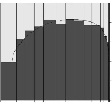
In campaining theory and voter targeting (e.g. Malchow [2008]), past voting behaviour of a person is considered to be the strongest predictor of future voting behaviour. Here, it is usually assumed that the more often a person went voting in the past, the more likely she is to do so in the upcoming election. Statistically this is a logistic regression problem with a binary dependent variable and therefore fits into the GLM framework. The number of attended elections was used as the predictor variable. It is important to note though, that the raw count of attended elections may be misleading because a higher count does not need to be the result of a general disposition to vote more likely. We therefore calculated the percentage of attended elections out of all elections a person was eligible to take part in to correct for possible bias. Figure 1 shows a spine plot of the data. It can be seen that the relationship is not monotonic but appears to be quadratic. This is not in accordance with intuition or the literature on voter targeting. One would expect a higher likelihood to vote for those who have a higher percentage of attended elections.

We fitted a global logistic regression modelM(Y,β) with a quadratic effect of the predictor variable,

g(µ) =β0+β1x+β2x2 (10)

where x is the percentage of attended elections (“percentAttended”). The estimated model parameters and goodness-of-fit values of the global model are displayed in Table 1. Interpola-tions of the predicted values were added to the spine plot in Figure 1. The initial observation could be confirmed by the model, the quadratic term turns out to be significant.

But why would people with a very high general attendance rate have a similarly low atten-dance rate in the 2004 election as people who usually will attend elections rarely? And what people are they? We employed recursive partitioning of the logistic regression model in (10) to see if additional variables can shed more light on this phenomenon. We used a significance level ofα = 0.05 for the generalized M-fluctuation tests and forced the minimum number of observations within each node to be at least 1600 (a fraction of about 8% of the overall data).

percentAttended gen04 0 5 10 15 20 25 30 35 40 45 50 60 1 0 0.0 0.2 0.4 0.6 0.8 1.0

Figure 1: Spineplot of relative voting frequencies against the percent of attended elections out of all elections a person was eligible to. The solid black line is the interpolated prediction from a logistic regression model with a quadratic term for the predictor “percentAttended”.

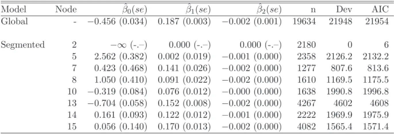
Table 1: Parameter estimates (standard errors in brackets) and goodness-of-fit statistics (de-viance and AIC) for the global logistic regression model and the terminal nodes of the segmented logistic regression model for the Ohio voter data.

Model Node βˆ0(se) βˆ1(se) βˆ2(se) n Dev AIC

Global - −0.456 (0.034) 0.187 (0.003) −0.002 (0.001) 19634 21948 21954 Segmented 2 −∞ (-.–) 0.000 (-.–) 0.000 (-.–) 2180 0 6 5 2.562 (0.382) 0.002 (0.019) −0.001 (0.000) 2358 2126.2 2132.2 7 0.423 (0.468) 0.141 (0.026) −0.002 (0.000) 1277 807.6 813.6 8 1.050 (0.410) 0.091 (0.022) −0.002 (0.000) 1610 1169.5 1175.5 10 −0.319 (0.084) 0.076 (0.012) −0.000 (0.000) 1638 1990.8 1996.8 13 −0.704 (0.058) 0.152 (0.008) −0.002 (0.000) 4267 4602 4608 14 0.161 (0.093) 0.122 (0.012) −0.001 (0.000) 2222 1969.9 1975.9 15 0.056 (0.140) 0.170 (0.013) −0.002 (0.000) 4082 1565.4 1571.4

The resulting tree is depicted in Figure 2 and the parameter estimates of the local models for the terminal nodes are given in Table 1.

The result from the partitioning algorithm shows what or who is responsible for the quadratic relationship between the percent of attended elections and the likelihood to vote. First there is a terminal node with people who did not vote at all. Please note that within this node we find quasi-complete separation1 [Albert and Anderson, 1984]. Second, the relation-ship is driven by the 5245 people whose household consists of people who are affiliated solely with the Democratic Party (node 5) and to a lesser extent by those affiliated solely with the Republican party (node 7) or whose household consists only of democrats and republicans (node 8). In other words, there are no independent voters in these households. Especially the segment of people whose household is composed entirely of Democrats (n5 = 2358) contribute to the overall quadratic relationship seen in Figure 1. They show declining voting probability for people with a high general individual turnout and quite strongly so. While those people with a small to medium percentage of general attendance have fairly high voting probabilities that slightly increase for higher predictor values, those with a general attendance rate of 0.85 or more (nearly half of the segment) experience a sheer drop of voting probability.

For the other two segments, those whose household consists entirely of Republicans or of a mix of Republicans and Democrats (n7 = 1277 and n8 = 1610), this picture is less striking. Here, an attendance rate of about 0.1 to 0.8 is associated with the highest voting probability, whereas very rare voters (x ≤0.1) and very frequent voters (x ≥0.85) have a similarly high voting probability that is slightly less than for the other people in the segment. Nodes 7 and 8 differ in the assigned rank in the household. The difference between these two nodes lies in the slightly higher overall voting probability and a higher probability for those with an attendance percentage between 25% and 80% for those with household ranks 1 and 2 (node 7).

On the other hand, the segments in terminal nodes 10, 13, 14 and 15 indeed show a

1

In this node the ML estimator does not exist. The algorithm has the positive effect to separate these observations from the rest, hence estimation in other nodes works well which would otherwise not be the case.

par tyMix p < 0.001 1 unkno wn {allR, allD , noneRorD , noneD , onlyRorD , noneR, allRorDorLegal} Node 2 (n = 2180) 0 25 1 0 0 0.2 0.4 0.6 0.8 1 ● ● ● ● par tyMix p < 0.001 3 {allR, allD , onlyRorD} {noneRorD , noneD , noneR, allRorDorLegal} par tyMix p < 0.001 4 allD {allR, onlyRorD} Node 5 (n = 2358) 0 25 88.235294117647 1 0 0 0.2 0.4 0.6 0.8 1 ● ● ● ● householdRank p < 0.001 6 ≤ 2 > 2 Node 7 (n = 1277) 0 25 88.235294117647 1 0 0 0.2 0.4 0.6 0.8 1 ● ● ● ● Node 8 (n = 1610) 0 25 88.235294117647 1 0 0 0.2 0.4 0.6 0.8 1 ● ● ● ● householdRank p < 0.001 9 ≤ 3+ > 3+ Node 10 (n = 1638) 0 25 1 0 0 0.2 0.4 0.6 0.8 1 ● ● ● ● par tyMix p < 0.001 11 noneRorD {noneD , noneR, allRorDorLegal} householdHead p < 0.001 12 H M Node 13 (n = 4267) 0 25 1 0 0 0.2 0.4 0.6 0.8 1 ● ● ● ● Node 14 (n = 2222) 0 25 1 0 0 0.2 0.4 0.6 0.8 1 ● ● ● ● Node 15 (n = 4082) 0 25 88.235294117647 1 0 0 0.2 0.4 0.6 0.8 1 ● ● ● ● F igur e 2: Th e re su lt in g tr ee st ru ct u re af ter p ar tit ion ing th e logis ti c regr essi on m o de l wi th li n ear p red ict or β0 + β1 x + β2 x 2 wi th x d en ot in g the re lat iv e fr eq ue nc y of at ten de d el ect ions , “p er cen tA tt en de d” . The ter mi nal s n o d es d isp la y spi n e pl ot s of the ob ser v ed re lat iv e fr eq ue nc ies agai n st th e at ten d ed p er ce n tage for eac h par ti tion wi th the sol id lin es con ne ct ing th e pr ed ict ed v al ue s from the logi st ic regr ess ion m o de l.

monotonically increasing voting probability for an increase of the predictor variable. This is in accordance with intuition and literature on political campaining. Here, having at least one household member who identifies herself as “independent” is the key difference to the segments with an inverse U-shaped voting probability relationship with the percentage of attended elections.

By using model-based recursive partitioning with additional covariate information, we were able to find an explanation as to why a quadratic effect has to be included into the logistic regression model. We could single out the observations that were responsible for this phe-nomenon and show that there are segments in which the assumed monotonic relationship is actually present.

3.2 Identifying Segments With Poor or Good Fit

Another area in which model-based recursive partitioning can be helpful is in identifying segments of the data for whom an a priori assumed structural model fits well. It may be that overall this model has a poor fit but that this is due to some contamination (for example merging two separate data files or systematic errors during data collection at a certain date). By using the described algorithm the data set might be partitioned in a way that enables us to find the segments that have poor fit and find segments for which the fit may be rather good.

To illustrate this, we use data of debt amortization rates as a function of the duration of the enforcement. It can be expected that the longer the enforcement lasts, the higher amortization rate should be achieved. What is special about these data is that they came from two sources and were merged into a single data set. The merged data set consisted of

n= 165 observations, with 75 observations from file 0 and 90 observations from file 1. The structure of the statistical problem here is similar to a “time-to-event” analysis. We consider the amortization rate relative to the original claim as the metric variable whose hazard function we want to model. Failure to pay more, default, insolvency, bankruptcy or meeting the obligation were considered as the event “stopped paying”. Additionally, we have the possibility of right censored observations if a person was lost to follow up. This led us to using a Weibull regression model which is an example of models described in Section 2.4. Here, the scale parameter and the parameters of the linear predictor are not orthogonal and have to be estimated simultaneously.

Formally, following Venables and Ripley [2002], we model the hazard functionh(r), withr

denoting a realisation of the random variable of achieved amortization rate, R, which takes the form of

h(r) =λααrα−1 =αrα−1exp(αβTx) (11)

for the Weibull distribution. The parameter λis modelled as an exponential function of the covariates x. In a loglinear model formulation this becomes

log(R) =−logλ+ 1

αlog (12)

withbeing a disturbance term that is independent ofxand w.l.g exponentially distributed. In this particular example,xconsists of an intercept and the duration of the enforcement.

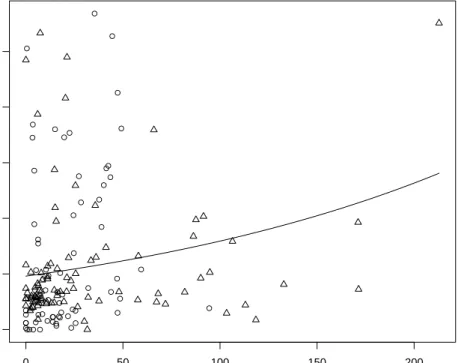
A visualisation of the data can be found in Figure 3. The chosen point type corresponds to the different files, a circle for file 0 and the triangle for file 1. Additionally we included the

● ● ● ● ● ● ● ● ● ● ● ● ● ● ● ● ● ● ● ● ● ● ● ● ● ● ● ● ● ● ● ● ● ● ● ● ● ● ● ● ● ● ● ●● ● ● ● ● ● ● ● ● ● ● ● ● ● ● ● ● ● ● ● ● ● ● ● ● ● ● ● ● ● ● 0 50 100 150 200 0.0 0.2 0.4 0.6 0.8 1.0 Duration of Enforcement Amor tization

Figure 3: Scatterplot of duration of the enforcement and the achieved amortization rate until the event failure to pay more” happened. The solid line represents the predicted values from the global Weibull regression model. Observations from file ”0” are plotted as circles, those from file ”1” as triangles.

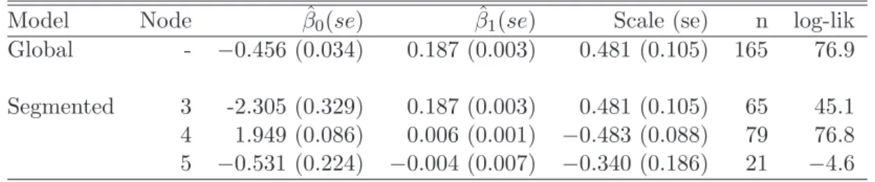
Table 2: Parameter estimates (standard errors in brackets) and goodness-of-fit statistics for the global Weibull model and the terminal nodes of the segmented Weibull model for the debt amortization data

Model Node βˆ0(se) βˆ1(se) Scale (se) n log-lik Global - −0.456 (0.034) 0.187 (0.003) 0.481 (0.105) 165 76.9 Segmented 3 -2.305 (0.329) 0.187 (0.003) 0.481 (0.105) 65 45.1 4 1.949 (0.086) 0.006 (0.001) −0.483 (0.088) 79 76.8 5 −0.531 (0.224) −0.004 (0.007) −0.340 (0.186) 21 −4.6

predicted values from the global Weibull regression model. The results of the model fitting procedure can be seen in Table 2.

What we can see here is that the global model does not fit well. The log-likelihood for the regression model was 76.9 and for the intercept only model it was 75.1 which is not significant at α = 0.05 (p = 0.054). Apart from that it looks as though the Weibull regression is not really appropriate for the whole data set. However, one can see that the bulk of the data may be appropriately modelled with the proposed relationship if it were not for the observations that have quite high amortization rates for a low enforcement duration. There are two possible explanations for such a lack of fit: (i) explanatory variables that were not considered in the model (misspecification) and (ii) data contamination. In this analysis it is quite likely that (i) has some effect. We will use information from other covariates in the subsequent recursive partitioning and gauge their influence. Inspection of Figure 3 however reveals something else. Observations that have high amortization rates for low duration time are mainly from file 0. Additionally the distribution of the enforcement duration in file 1 is more skewed (1.96 vs. 1.39) and has a much longer right tail. The same holds for the amortization rate. It looks as if merging the two data sets led to a contamination, as they are probably not comparable.

We partitioned these based on the Weibull regression model from (11). As additional covariates that were used for partitioning we had the persons gender, liability at the begin of the enforcement, the current liability, the number of securities a person had as well as a person’s collateralization ratio. We also included a dummy variable to flag which file the observation was from.

The resulting tree can be found in Figure 4 and the estimated model in Table 2. We see that both suspicions from above can be confirmed. First, there is an additional variable, collateralization ratio, that leads to a segment where the influence of the duration is not significant. This is partly due to the small sample size in this node, but we can also see that the regression coefficient has a negative sign. It does not appear as if there would be a positive relationship that we just did not detect but rather that there is no positive relationship at all. This makes sense, as the collateralization ratio gives a good measure of how many and how well diversified the securities of a person are and how high their value is. A person with a high collateralization ratio (two cars for example) may be able to amortize her debt very fast or at least it may not depend on the duration of the enforcement. It seems rather likely that a person with a high collateralisation ratio who does not amortize her debt rather soon may have problems with or may refuse payment regardless of enforcement duration.

collatRatio p < 0.001 1 ≤ 0.11 > 0.11 file p = 0.021 2 0 1 Node 3 (n = 65) ● ● ● ● ● ● ● ● ● ● ● ● ● ● ● ● ● ● ● ● ● ● ● ● ● ● ● ● ● ● ● ● ● ● ● ● ● ● ● ● ● ● ● ● ● ● ● ● ● ● ● ● ● ● ● ● ● ● ● ● ● ● ● ● ● −6.9 102 0 1 Dur ation Achieved amor tization Node 4 (n = 79) ● ● ● ● ● ● ● ● ● ● ● ● ● ● ● ● ● ● ● ● ● ● ● ● ● ● ● ● ● ● ● ● ● ● ● ● ● ● ● ● ● ● ● ● ● ● ● ● ● ● ● ● ●●●●●● ● ● ● ● ● ● ● ● ● ● ● ● ● ● ● ● ● ● ● ●● −6.9 219.8 0 1 Dur ation Achieved amor tization Node 5 (n = 21) ● ● ● ● ● ● ● ● ● ● ● ● ● ● ● ● ● ● ● ● ● −6.9 102 0 1 Dur ation Achieved amor tization F igur e 4: Th e rec ur siv ely p art it ione d W eib u ll regr es si on m o de l of amor ti zat ion rat e exp lai ne d b y th e d ur at ion of the en for ce men t. F or eac h te rm inal n o de the re is a sc at ter pl ot wi th th e sol id li ne re pr esen ti ng th e p red ic ted v alu es fr om th e m o de l.

to a difference in the two data sources. For one data set, file 1, the Weibull regression actually fits rather well (node 4, log-likelihood of 76.8). Additionally, we have a significant positive influence of the explanatory variable. Please note however, that the coefficient and corresponding p-value is highly influenced by a outlier with amortization rate greater than 1. Removing this value leads to a much weaker association that is barely significant on a 5% level 2. In node 3, for which all observations stem from file 0, we see an ill fit of the Weibull model with a log-likelihood of 45.1. It even looks as if the (significant) regression line is splitting the data in this node into two groups rather than explaining them. There seems to be unexplained heterogeneity in the data in this segment that cannot be explained by the regression model.

What we can see from this analysis however is that recursive partitioning of models can help us identify segments in our data for which the model may either fit well or may be inap-propriate. Here, merging to data from file 0 with those in file 1 leads to contamination of the merged data set. This contamination masks the acceptable fit for the subset of observations from file 1, a fact that is not necessarily clear from the non-segmented analysis. Most proba-bly those two data sets were obtained individually and on different occassions or for different studies. They just happen to have similar variables in them. This goes to show once again that planning a study involves more than just collecting data.

4 Discussion

In this paper, we introduced recursive partitioning of generalized linear models as a special case of model-based recursive partitioning. We tried to illustrate how the algorithmic ap-proach may lead to additional insight for ana priori assumed parametric model, especially if the underlying mechanisms are too complex to be captured by the GLM. As such model-based recursive partitioning can automatically detect interactions, non-linearity, model misspecifi-cation, unregarded covariate influence and so on. As an exploratory tool, it can be used for complex and large data sets for which a globally fitted GLM runs into problems. Compared to fully non-paramteric tree algorithms on the other hand, the specification of a parametric model in the terminal nodes can add extra stability and therefore reduce the variance of those tree methods. This is because functional trees tend to be smaller and the functional restrictions provide additional stability. Being a hybrid of trees and classic GLM, their per-formance usually lies between those two poles: They tend to exhibit higher predictive power than classic models but less than non-parametric trees [Zeileis et al., 2008]. They add some complexity compared to classical model because of the splitting process but are usually more parsimonous than non-parameteric trees. They show a slightly higher variance than a classic model in bootstrap experiments, but much less than in non-parametric trees (even pruned ones). We believe that the exploratory use of recursive partitioning of GLM is fruitful for researchers dealing with GLM to detect additional patterns and get a better grasp of what is really happening in the data at hand, especially if a classical statistical modelling approach runs into problems.

2

References

Aitkin, M., Francis, B., Hinde, J., and Darnell, R. (2009). Statistical Modelling in R. Oxford University Press, Inc., New York.

Albert, A. and Anderson, J. A. (1984). On the existence of maximum likelihood estimates in logistic regression models. Biometrika, 71:1–10.

Andrews, D. (1993). Tests for parameter instability and structural change with unknown change point. Econometrica, 61:821–856.

Breiman, L., Friedman, J. H., Olshen, R. A., and Stone, C. J. (1984). Classification and Regression Trees. Wadsworth, California.

Chan, K. and Loh, W. (2001). LOTUS. an algorithm for building accurate and comprehensible logistic regression trees. Journal of Computational and Graphical Statistics, 13:826–852. Choi, Y., Ahn, H., and Chen, J. (2005). Regression trees for analysis of count data with extra

poisson variation. Computational Statistics & Data Analysis, 49:893–915.

Clarke, B., Fokoue, E., and Zhang, H. H. (2009). Principles and Theory of Data Mining and Machine Learning. Springer, New York.

Gama, J. (2004). Functional trees. Machine Learning, 55:219–250.

Hastie, T., Tibshirani, R., and Friedman, J. (2009).Elements of Statistical Learning. Springer, New York, 2nd ed. edition.

Hjort, N. and Koning, A. (2002). Tests for constancy of model parameters over time. Non-parametric Statistics, 14:113–132.

Hochberg, Y. and Tamhane, A. C. (1987). Multiple Comparison Procedures. John Wiley & Sons, New York.

Hothorn, T., Hornik, K., and Zeileis, A. (2006). Unbiased recursive partitioning: A conditional inference framework. Journal of Computational and Graphical Statistics, 15(3):651–674. Huber, P. (2009). Robust Statistics. John Wiley & Sons, Hoboken, NJ, 2nd edition.

Kim, H. and Loh, W. (2001). Classification trees with unbiased multiway splits. Journal of the American Statistical Association, 96:589–604.

LeCam, L. (1990). Maximum likelihood - an introduction. ISI Review, 58(2):153–171. Loh, W. (2002). Regression trees with unbiased variable selection and interaction detection.

Statistica Sinica, 12:361–386.

Loh, W. and Shih, Y. (1997). Split selection methods for classification trees.Statistica Sinica, 7:815–840.

Malchow, H. (2008). Political Targeting. Predicted Lists, LLC, 2nd ed., edition.

McCullagh, P. and Nelder, J. (1989).Generalized Linear Models. Chapman and Hall, London, 2nd ed., edition.

Morgan, J. and Sonquist, J. (1968). Problems in the analysis of survey data, and a proposal.

Journal of the American Statistical Association, 58:415–434.

Quinlan, J. R. (1993). C 4.5: Programs for Machine Learning. Morgan Kaufmann Publ., San Mateo, California.

Rao, C. R. and Toutenburg, H. (1997).Linear Models: Least Squares and Alternative Methods. Springer, New York, 2nd ed., edition.

Su, X., Wang, M., and Fan, J. (2004). Maximum likelihood regression trees. Journal of Computational and Graphical Statistics, 13:586–598.

Venables, W. N. and Ripley, B. D. (2002). Modern Applied Statistics with S. Springer, New York, 4th ed., edition.

White, H. (1982). Maximum likelihood estimation of misspecified models. Econometrica, 29:1–25.

Zeileis, A. (2005). A unified approach to structural change tests based on ML scores, F

statistics, and OLS residuals. Econometric Reviews, 24(4):445–466.

Zeileis, A. and Hornik, K. (2007). Generalized M-fluctuation tests for parameter instability.

Statistica Neerlandica, 61(4):488–508.

Zeileis, A., Hothorn, T., and Hornik, K. (2008). Model-based recursive partitioning. Journal of Computational and Graphical Statistics, 17(2):492–514.

Zhang, H. and Singer, B. H. (2010). Recursive Partitioning and Applications. Springer, New York, 2nd ed., edition.