Optimal realisations of fixed point implemented digital controller with the smallest dynamic range

Vol. 79, No. 10, October 2006, 1297–1312

Optimal realizations of fixed-point implemented digital

controllers with the smallest dynamic range

J. WUy, S. CHEN*z, G. LIx

and J. CHUy

yNational Key Laboratory of Industrial Control Technology, Institute of Advanced Process Control, Zhejiang University, Hangzhou, 310027, P.R. China

zSchool of Electronics and Computer Science, University of Southampton, Highfield, Southampton SO17 1BJ, U.K.

xSchool of Electrical and Electronic Engineering, Nanyang Technological University, Singapore

(Received 19 August 2005; in final form 7 November 2005)

A novel approach is proposed to design optimal finite word length (FWL) realizations of digital controllers implemented in fixed-point arithmetic. A minimax-based search procedure is first formulated to obtain an optimal controller realization that optimizes an FWL closed-loop stability measure. Since this FWL closed-loop stability measure is solely linked to the fractional part or precision of fixed-point format, the resulting realization may not have the smallest dynamic range. A measure is then derived to indicate the dynamic range of fixed-point implemented realization. By choosing an appropriate orthogonal transformation of this dynamic range measure of the optimal precision controller realization, a numerical optimization method is developed to make the controller realization having the smallest dynamic range without sacrificing FWL closed-loop stability robustness. The proposed approach is more efficient than a direct optimization of some combined FWL closed-loop stability and dynamic range measure via a numerical means. The proposed approach is established within a unified framework that includes both the shift and delta operator parameterizations, which makes it possible to compare the closed-loop stability characteristics of the optimal FWL controller realizations using shift and delta operators, respectively. Through analysing the simulation results of a design example, some useful insights and understandings are obtained regarding the FWL controller realizations based on shift and delta operators.

1. Introduction

In a closed-loop control system, there generally exist two kinds of uncertainty which have detrimental effects on the system performance. The first is the uncertainty within the plant. This kind of uncertainty has been extensively studied, and some effective methods, such as

H1 method (Zhouet al. 1996) and l1method (Dahleh and Diaz-Bobillo 1995), have been established to design controllers which are capable of dealing with the plant uncertainty. When a designed control law is implemen-ted, the second kind of uncertainty, the uncertainty within the controller, arises. It is well-known that,

in practice, a controller cannot be implemented exactly. For example, when a control law is digitally implemen-ted using a digital processor of finite word length (FWL), the finite-precision representation of the con-troller parameters is the main source of concon-troller uncertainty. In comparison with the plant uncertainty, this controller uncertainty is small. This is the reason why the classical controller design methodology has ignored the controller uncertainty. However, it has increasingly been realized that the controller uncertainty due to the FWL effect cannot be ignored (Liu et al. 1992, Gevers and Li 1993, De Oliveira and Skelton 2001, Istepanian and Whidborne 2001). Firstly, for many industrial and mass-market consumer applications, a fixed-point implementation of digital controller is desired for its advantages in cost, simplicity, speed, *Corresponding author. Email: [email protected]

International Journal of Control

ISSN 0020–7179 print/ISSN 1366–5820 onlineß2006 Taylor & Francis http://www.tandf.co.uk/journals

memory space and power consumption. With a fixed-point processor, however, the detrimental FWL effects are markedly increased due to a reduced precision. Secondly, some canonical controller realizations are inherently ill-conditioned, and a small error will rapidly accumulate, subsequently degrading the designed loop performance and even resulting in closed-loop instability. Furthermore, modern control design methods result in controllers of high order, where such FWL effects are even more pronounced, as is high-lighted in the so-called fragility puzzles (Keel and Bhattacharryya 1997). Thus it is imperative that great care must be exercised when implementing digital controllers.

As the first and the most critical requirement for a closed-loop control system is its stability, most researches in digital controller implementation have focused on the FWL effects on closed-loop stability (Fialho and Georgiou 1994, Li 1998, Chenet al. 1999, Whidborne et al. 2000a, 2001, Fialho and Georgiou 2001, Wu et al. 2001). A basic idea underpinning all these researches follows. There exist an infinite number of different realizations corresponding to a control law. Although these controller realizations are equivalent, if infinite-precision implementation can be assumed, they are no longer equivalent under practical finite-precision implementation. It is recognized that, subject to the FWL effect, certain controller realizations exhibit superior ‘‘robustness’’ of closed-loop stability, com-pared to others. This observation can be utilized to select ‘‘optimal’’ realizations that optimize some given FWL closed-loop stability measures. Various FWL closed-loop stability measures have been investigated, and these include the complex stability radius measure (Fialho and Georgiou 2001, Chenet al. 2002), a variety of pole sensitivity measures (Mantey 1968, Li 1998, Chenet al. 1999, Whidborneet al. 2001, Wuet al. 2001) and the l1 based stability measure (Whidborne et al. 2000a). This approach has also been extended to study the closed-loop stability issues of FWL controller realizations using the delta operator formulation (Chen

et al. 2000, Wu et al. 2000). All these measures in the previous works, designed for fixed-point implementa-tion, have a limitation in that they are only linked to the fractional part of fixed-point representation. Optimizing these measures, while minimizing the bits required for the fractional part, may actually increase the integer part or dynamic range of fixed-point representation. Thus, the resulting ‘‘optimal’’ controller realizations are not necessarily true optimal ones in terms of the robustness to the FWL effects.

In a fixed-point implementation, the total available bits have to accommodate the dynamic range first to avoid overflow, and the remaining bits left are then used to implement the fractional part. Therefore, a

better approach to design optimal fixed-point controller realizations is to consider both a precision or FWL closed-loop stability measure and a dynamic range measure together. In a recent study (Wu et al. 2003), this approach is adopted for fixed-point, floating-point or block-floating-point implemented digital controllers. A potential drawback of this previous approach is high computational complexity, particularly for high-order controllers. This is because numerical methods have to be used which can only rely on function values for optimization search. In this study, we adopt a very different ‘‘two-procedure’’ approach. Firstly, we opti-mize the FWL closed-loop stability measure proposed by Li (1998) to obtain an optimal realization. Secondly, we then optimize a dynamic range measure for this optimal realization. This second-step is based on an invariant property of the controller realization under orthogonal transformation. It is known that the value of the FWL closed-loop stability measure is invariant under an orthogonal transformation of controller realization (Gevers and Li 1993) and this property was utilized by Gevers and Li (1993) to obtain sparse realizations. We exploit this extra freedom of realization to minimize the dynamic range of the controller realization.

This two-procedure approach is attractive for the following reasons. In the first procedure, the minimax theorem and subgradient algorithms are used to search for a global optimal solution of the given FWL closed-loop stability measure (Wuet al. 2002). Thus, provided that there are sufficient bits for accommodating the dynamic range, the realization obtained is global optimal and is most robust to the FWL effect. In the second procedure, based on an appropriate orthogonal transformation, numerical optimization is carried out in a much smaller space than the full realization space, and the resulting realization remains to be an optimal realization with respect to the first-procedure measure. That is, the final realization has the smallest dynamic range under the constraint that it also has the maximum FWL stability robustness. The proposed approach is established in a unified framework for both the shift and delta operators to enable a comparison for the FWL closed-loop stability characteristics of the optimal controller realizations using these two operators.

In x4, a criterion is introduced which measures the dynamic range of a fixed-point realization, and a method is developed to minimize this dynamic range criterion over the set that contains all the orthogonal transformations of the optimal realization obtained using the procedure described in the previous section. A comparison with a direct numerical optimization of the combined FWL closed-loop stability and dynamic range measure (Wu et al. 2003) is also given in this section. Inx5, a design example is used to demonstrate the effectiveness of the proposed optimization strategy and to compare the FWL closed-loop stability char-acteristics of optimal controller realizations using the shift and delta operators. The simulation results are analysed to reveal useful insights to these two different operator parameterizations of controller. The paper concludes inx6.

2. Notations and the problem formulation

Let R denote the field of real numbers, C the field of complex numbers, andeitheith real coordinate vector. For anyz2 Cn, define

ðzÞ ¼ ½<ðzÞ =ðzÞÞ, ð1Þ

where<ðzÞ and=ðzÞdenote the real and the imaginary parts of z, respectively. For a complex-valued matrix

U2 Cmn with elements uij, we define the following matrix norms

kUk_M¼ max i2 f1,...,mg

j2 f1,...,ng

juijj, ð2Þ

kUk_F ¼

ffiffiffiffiffiffiffiffiffiffiffiffiffiffiffiffiffiffiffiffiffiffiffiffiffi Xm

i¼1 Xn

j¼1 juijj2

v u u

t : ð3Þ

Let Vec() be the column stacking operator such that Vec(U) is anmn-dimenstional vector. As usual,UTis the transposed matrix of U, UH is the Hermitian adjoint matrix ofU, andU* is conjugate toU. For a real-valued square matrix M2 Rnn, let fliðMÞ, 1ing denote its eigenvalues, and let xi(M) be the right eigenvector corresponding to li(M). If M is diagonalizable, the matrix

Mx¼ ½x1ðMÞ x2ðMÞ xnðMÞ ð4Þ

is invertible. Define

My¼ y1ðMÞ y2ðMÞ ynðMÞ

¼ M_xH ð5Þ

where yi(M) is called the reciprocal left eigenvector corresponding toxi(M).

A discrete-time linear system can be described using either the usual forward shift operatorzor the so-called delta operator. The latter is defined as (Middleton and Goodwin 1990)

¼ z1

h ð6Þ

where h is a positive real constant (the constant h is originally limited to the sampling period by Middleton and Goodwin (1990) but this constraint is removed by Gevers and Li (1993)). In this paper, it is assumed that the value ofhin theoperator has an exact fixed-point representation (e.g.h¼22orh¼26) so that the source of FWL errors comes solely from a finite-precision implementation of the controller realization. For the notational conciseness and to avoid separate derivations for the two operators, we introduce a ‘‘generalized’’ operatorfor the discrete-time system. It is understood that¼zor, depending on which operator is actually used. The state-space description of the general discrete-time system using the generalized operatoris

xgðkÞ ¼Fg,xgðkÞ þGg,ug,1ðkÞ þHg,ug,2ðkÞ y_gðkÞ ¼Jg,xgðkÞ þMg,ug,1ðkÞ,

(

ð7Þ

where all the matrices and vectors are real-valued with appropriate dimensions. Obviously,¼zand¼give rise to the two equivalent representations of the same system, with the following relationship

Fg,¼

Fg,zI

h , Gg, ¼ Gg,z

h , Jg,¼Jg,z, Mg,¼Mg,z, Hg,¼

Hg,z

h , ð8Þ

where I denotes the identity matrix of appropriate dimension. In particular, the operator z is interpreted aszxgðkÞ ¼xgðkþ1Þ. The following theorem relates the eigenvalues ofFg,zto those ofFg,.

Theorem 1: With a proper index order, {li(Fg,z)} and {li(Fg,)}can be one-to-one mapped with

liðFg,zÞ ¼1þhliðFg,Þ, 8i: ð9Þ

It is well known that the discrete-time system (Fg,z, Gg,z,

Jg,z,Mg,z,Hg,z)is stable if and only if

jliðFg,zÞj<1, 8i: ð10Þ

From Theorem1,we have the stability condition for the same system described usingoperator.

Theorem 2: The discrete-time system (Fg,, Gg,, Jg,,

Mg,,Hg,)is stable if and only if

liðFg,Þ þ

1

h

<1

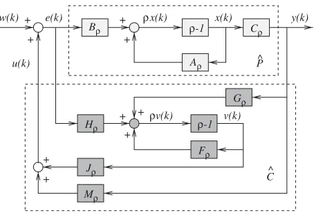
Now consider the discrete-time closed-loop control system depicted in figure 1, where the linear time-invariant plant P^ is described by the state-space description

xðkÞ ¼AxðkÞ þBeðkÞ

yðkÞ ¼CxðkÞ

ð12Þ

which is completely state controllable and observable with A2 Rnn, B2 Rnp and C2 Rqn; and the

generic digital stabilizing controllerC^is described by the state-space description

vðkÞ ¼FvðkÞ þGyðkÞ þHeðkÞ

uðkÞ ¼JvðkÞ þMyðkÞ

ð13Þ

with F2 Rmm, G2 Rmq, J2 Rpm, M 2 Rpq

and H 2 Rmp. The generic controller structure in

figure 1 unifies the output feedback and observer-based controllers: C^ is an output feedback controller when

H¼0; a full-order observer-based controller when

F¼AGC, M¼0 and H¼B; a reduced-order

observer-based controller, otherwise (Kailath 1980, O’Reilly 1983).

According to a basic property of the linear system, the state-space descriptions or realizations (F, G, J,

M, H) of the controllerC^ are not unique. In fact, let

(F0, G0, J0, M0, H0) be a realization of C^ that

has been designed using a standard controller design procedure. Then all the realizations of C^ form a realization set

S¼

ðF,G,J,M,HÞ:F¼T1 F0T,G¼T1 G0, J¼J0T,M¼M0,H¼T1 H0

ð14Þ

where T2 Rmm is any real-valued non-singular

matrix, called a transformation. Any two realizations

inSpare completely equivalent if they are implemented with infinite precision. Define

w¼

VecðFÞ

VecðGÞ

VecðJÞ

VecðMÞ

VecðHÞ

2 6 6 6 6 6 6 4

3 7 7 7 7 7 7 5

, w0¼

VecðF0Þ

VecðG0Þ

VecðJ0Þ

VecðM0Þ

VecðH0Þ 2

6 6 6 6 6 6 4

3 7 7 7 7 7 7 5

: ð15Þ

We also refer to was a realization of C^. The stability

of the closed-loop control system depicted in figure 1 depends on the eigenvalues of the transition matrix

AðwÞ ¼

AþBMC BJ

GCþHMC FþHJ

¼ I 0

0 T1 " #

AþBM0C BJ0 G0CþH0M0C F0þH0J0

I 0

0 T

¼ I 0 0 T1 " #

Aðw0Þ I 0 0 T

, ð16Þ

where 0 denotes the zero matrix of appropriate dimension. Define the stability margin ofliðAðwÞÞas

SMðliðAðwÞÞÞ ¼

1 jliðAðwzÞÞj, if¼z, 1

h jliðAðwÞÞ þ

1

h, if¼: 8

< :

ð17Þ

From the fact that the closed-loop system is designed to be stable, it follows

SMðliðAðwÞÞÞ ¼SMðliðAðw0ÞÞÞ>0, 8i2 f1,. . .,mþng ð18Þ

which implies that all the different controller realizations

w2 S have exactly the same set of the closed-loop

eigenvalues if they are implemented with infinite precision.

In practice, however, a controller realization can only be implemented with finite precision. When w is

implemented using a fixed-point processor of the bit lengthb, bbits are assigned as follows. One bit is used for the sign,bgbits are used for the integer part of the representation, and the remainingbf¼bbg1 bits are used to implement the fractional part of the representa-tion. In order to avoid overflow in representing w, bg should be sufficiently large such that

kwkM2bg: ð19Þ

+

+ +

+ +

u(k)

B_ρ e(k)

A_ρ

+ Cρ

x(k)

J_ρ +

+

+ w(k)

P^

C y(k)

G_ρ

v(k)

F_ρ H_ρ

M_ρ

^ ρ-1

ρv(k) x(k)

ρ

ρ-1

Note that kwkM represents the dynamic range of w

in fixed-point format. Even assuming no overflow,wis

perturbed into wþ" due to the finite bf bits in the fractional part representation. It can easily be shown that each element of"is bounded by2ðbfþ1Þ_{, that is,}

k"kM 2ðbfþ1Þ: ð20Þ

With the perturbation ", liðAðwÞÞ is moved

toliðAðwþ"ÞÞ. If an eigenvalue ofAðwþ"Þ crosses

over the stability boundary, the closed-loop system, originally designed to be stable, becomes unstable. Under the condition of no overflow, it can be seen that the closed-loop stability depends only on the perturbation ", that is, the accuracy or precision of the fractional part representation.

Intuitively, different controller realizations have different degrees of robustness to the FWL effect. It is highly desired to be able to quantify how robust a controller realization is in terms of its closed-loop stability under FWL implementation and to find some optimal realization that has the maximum robustness to the FWL effect. Because the total bit length b is divided between the dynamic range and precision of fixed-point format, this is a multi-objective optimi-zation. Firstly, an optimal realization should optimize some FWL closed-loop stability measure. Note that the value of such a stability measure only depends on the precision or fractional part of a controller realization. Secondly, a desired realization should also have the smallest dynamic range, since this will require the smallest number of bg bits to avoid overflow and in turn leaves the most bf bits to achieve the highest possible precision. In this study, we will adopt an effective two-procedure approach to tackle this multi-objective optimization problem.

3. Optimizing an FWL closed-loop stability measure

In the remainder of this paper, li is used to replace liðAðwÞÞ when doing so does not cause ambiguity.

Under the condition of no overflow, how easily the FWL error " can cause a stable control system to become unstable is determined by how much the stability margin each eigenvaluelihas and how sensitive the closed-loop eigenvalues are to the controller param-eter perturbations. The following FWL closed-loop stability measure, defined by Li (1998), is considered in this study. We adopt the inverse of the measure (thus the objective is to minimize) and remove the constant_ffiffiffiffi

N p

given by Li (1998).

fðwÞ ¼ max

i2 f1,...,mþng

k@li=@wkF

SMðliÞ

: ð21Þ

The measuref(w) describes the ‘‘robustness’’ of

closed-loop stability of the FWL perturbation " for the realization w. Since different controller realizationsw

have different values of f(w), it is natural to search

for ‘‘optimal’’ controller realizations that minimize the measure defined in (21). This leads to an optimal FWL controller realization problem

¼ min w2 S

fðwÞ: ð22Þ

Define

gðw,iÞ ¼

k@li=@wkF

SMðliÞ

: ð23Þ

Obviously, the optimization problem (22) can be viewed as

¼ min w2 S

max

i2 f1,...,mþnggðw,iÞ: ð24Þ

The following results (Owen 1982, Sze´p and Forgo´ 1985) on saddle points play an important role in obtaining global optimal solutions of minimax-formulation problems.

Definition 1: ðw0

,i0Þ 2 S f1,. . .,mþngis said to be

a saddle point ofg(w,i) if

gðw0

,iÞ gðw

0

,i

0_{Þ gðw}

,i0Þ, 8w2 S,

8i2 f1,. . .,mþng: ð25Þ

The next theorem is the well-known minimiax theorem in game theory.

Theorem 3: If and only if there exists at least a saddle pointðw0

,i0Þof g(w,i),then

min w2 S

max

i2 f1,...,mþnggðw,iÞ ¼i2 ð1,max...,mþngwmin2 Sp gðw,iÞ

¼gðw0

,i0Þ: ð26Þ

Theorem 4: Let i¼ min

w2 S

gðw,iÞ 8i2 f1,. . .,mþng, ð27Þ

i0¼ arg max

i2 f1,...,mþngi, ð28Þ

W ¼ w:gðw,i0Þ ¼i0,w 2 S

: ð29Þ

Then ðw0

,i0Þ is a saddle point of g(w, i) if and only if

w0

2 W and

gðw0,iÞ i0, 8i 2 f1,. . .,mþngnfi0g: ð30Þ

For closed-loop system with the forward shift operatorz

the procedure is extended into the generalized operator and the generic controller (13). The proposed search procedure, which consists of two stages, is outlined as follows.

3.1 Optimizing single-pole FWL stability measure

Given the realization w0, from the definition (14)

and (15), w actually depends on the

transforma-tion matrix T. In addition, SM(li) is fixed for given li. Thus, to attain the single-pole measure i defined in (27) for the eigenvalue li is equivalent to solve the minimization problem of the single-pole sensitivity

min

T2 Rmdet Tm6¼0 @li

@w

2

F

:

ð31Þ

The following lemma is due to Li (1998).

Lemma 1: Let the square matrix A¼M0þM1XM2 be diagonalizable where the real-valued matricesM0,M1 and M2 have proper dimensions and are independent of the real-valued matrixX.Then

@liðAÞ

@X ¼M

T

1y

iðAÞx T iðAÞM

T

2: ð32Þ

From (16), it can be seen that

AðwÞ ¼

AþBMC BJ

GCþHMC HJ

þ 0

I

F 0 I

,

ð33Þ

AðwÞ ¼

AþBMC BJ

HMC FþHJ

þ 0 I

G C 0

,

ð34Þ

AðwÞ ¼

AþBMC 0

GCþHMC F

þ B H

J 0 I

,

ð35Þ

AðwÞ ¼

A BJ

GC FþHJ

þ B H

M C 0

,

ð36Þ

AðwÞ ¼

AþBMC BJ

GC F

þ 0 I

H MC J

:

ð37Þ

Applying Lemma 1 to (33)–(37) gives rise to

@li

@F

¼0 Iy_iðAðwÞÞxTiðAðwÞÞ

0 I

, ð38Þ

@li

@G

¼0 Iy_iðAðwÞÞxTiðAðwÞÞ

CT I " #

, ð39Þ

@li

@J

¼hBT HTiy_iðAðwÞÞxTiðAðwÞÞ

0 I

, ð40Þ

@li

@M

¼ BT HT

h i

y_iðAðwÞÞxTiðAðwÞÞ

CT 0 " #

, ð41Þ

@li

@H

¼0 Iy_iðAðwÞÞxTiðAðwÞÞ

CTMT JT " #

: ð42Þ

8i2 f1,. . .,mþng, partition the eigenvectors ofAðw0Þ,

xiðAðw0ÞÞandyiðAðw0ÞÞ, into

xiðAðw0ÞÞ ¼

xi,1ðAðw0ÞÞ xi,2ðAðw0ÞÞ " #

, y_iðAðw0ÞÞ ¼

y_i,1ðAðw0ÞÞ y_i,2ðAðw0ÞÞ " #

,

ð43Þ

where xi,1ðAðw0ÞÞ, yi,1ðAðw0ÞÞ 2 Cn and xi,2ðAðw0ÞÞ,

y_i,2ðAðw0Þ 2 Cm. It is easy to see from (16) that,

8i2 f1,. . .,mþng,

xiðAðwÞÞ ¼

xi,1ðAðw0ÞÞ T1 xi,2ðAðw0ÞÞ

" #

,

y_iðAðwÞÞ ¼

y_i,1ðAðw0ÞÞ TTy_i,2ðAðw0ÞÞ

" #

: ð44Þ

Applying (44) to (38)–(42) results in

@li

@F

¼TTy_i,2ðAðw0ÞÞxiT,2ðAðw0ÞÞTT, ð45Þ

@li

@G

¼TTy_i,2ðAðw0ÞÞxTi,1ðAðw0ÞÞCT, ð46Þ

@li

@J

¼ BTy_i,1ðAðw0ÞÞ þHT0y

i,2ðAðw0ÞÞ

xT_i,2ðAðw0ÞÞTT,

ð47Þ

@li

@M

¼ BTy_i,1ðAðw0ÞÞ þHT0y

i,2ðAðw0ÞÞ

xT_i,1ðAðw0ÞÞCT,

ð48Þ

@li

@H

¼TTy_i,2ðAðw0ÞÞ

xT_i,1ðAðw0ÞÞCTM

T

0þx

T

i,2ðAðw0ÞÞJT0

Let

2_i ¼ kCpxi,1ðAðw0ÞÞk2Fþ kM0Cxi,1ðAðw0ÞÞ

þJ0xi,2ðAðw0ÞÞk2F, ð50Þ

2_i ¼ kBTy_i,1ðAðw0ÞÞ þHT0yi,2ðAðw0ÞÞk2F, ð51Þ

2_i ¼kBTyi,1ðAðw0ÞÞ þHT0yi,2ðAðw0ÞÞk2FkCxi,1ðAðw0ÞÞk2F,

ð52Þ

q_i¼ xi,2ðAðw0ÞÞ, ð53Þ

zi¼ yi,2ðAðw0ÞÞ: ð54Þ

Then @li @w 2 F

¼ @li @F

2

F

þ @li @G

2

F

þ @li @J

2

F

þ @li @M

2

F

þ @li @H

2

F

¼ kT1 q_ik2_FkTTzik2Fþ2ikTTzik2F

þ2_ikT1 q_ik2_Fþ_i2: ð55Þ

For the different cases of qi and zi, the results on minimizing k@li=@wk2F and the related proofs are given in Wuet al. (2005). Based on these results, all the solutions to (27) can be specified. The following theorem lists the result for one case ofqiandzito illustrate how the problem is solved.

Theorem 5: Given positive i,i2 R, qi,zi2 Cm and detðððziÞÞTðqiÞÞ>0,we have

min T2 Rmm

detT6¼0

@li

@w

2

F

¼ jzH_i q_ij þii

2

2_i2_i þ2_i, ð56Þ

andk@li=@wk2F achieves the minimum if and only if

T¼Q

H1=2 0 FðH1=2ÞT :

" #

V ð57Þ

where the orthogonal matrixQcan be obtained from the QR factorization ofðziÞ

ðziÞ ¼Q

11 12

0 22

0 0 .. . 0 .. . 0 2 6 6 6 6 6 6 4 3 7 7 7 7 7 7 5

ð58Þ

with non-zero11,22 2 R,

H¼ i i

11 12

0 22

T

ððziÞÞTðqiÞ

cos sin

sin cos

11 12

0 22

1

ð59Þ

F¼ i i eT 3 .. . eT m 2 6 6 4 3 7 7

5QTðqiÞ

cos sin

sin cos

11 12

0 22

1

,

ð60Þ

is the solution of

tan ¼a21a12 a11þa22 a11cos a12sin >0 8

<

: ð61Þ

with

a11 a12 a21 a22

¼ ððziÞÞTðqiÞ, ð62Þ

2 Rðm2Þðm2Þis an arbitrary non-singular matrix,and V2 Rmm is an arbitrary orthogonal matrix.

3.2 Global optimal controller realizations

In x3.1, the problem of attaining the single-pole FWL stability measure i is solved and hence the index i0 is readily given from i0¼max_{i2 f1,...,mþngi}. Without the

loss of generality, it is assumed that li0 is a

complex-valued eigenvalue and detðððzi0ÞÞTðq

i0ÞÞ>0. From

Theorem 5, all the transformation matrices achieving i0 form the set

T ¼ TT¼Q

H1=2 0 FðH1=2ÞT :

" # V ) (

ð63Þ

whereQ,HandFare determined according toi0,_i0,q

i0, zi0 as well as Theorem 5,2 Rðm2Þðm2Þis an arbitrary

non-singular matrix and V2 Rmm is an arbitrary orthogonal matrix. The realization set W defined in (29) is described on the transformation setT as

W ¼ w:w¼wðTÞ ¼

VecðT1 F0TÞ

VecðT1 G0Þ

VecðJ0TÞ

VecðM0Þ

VecðT1 H0Þ 2 6 6 6 6 6 6 4 3 7 7 7 7 7 7 5

,T2 T

8 > > > > > > < > > > > > > : 9 > > > > > > = > > > > > > ; :

ð64Þ

From (23), (55) and the definition ofkkF, it can be seen that gðwðTÞ,iÞ ¼gðwðTVÞ,iÞ for any orthogonal

that V plays no role in computing g(w, i) and hence

we simply setV¼Iin this section. Therefore

T¼Tð:Þ ¼Q

H1=2 0 FðH1=2ÞT :

" #

, ð65Þ

are explored for a non-singularopt 2 Rðm2Þðm2Þsuch

thatgðwðTð:optÞÞ,iÞ i0,8i. We can seek_optusing

a subgradient algorithm presented in Wu et al. (2005). The basic steps of this subgradient algorithm is listed here for completeness.

Initialization: Arbitrarily select a non-singular

2 Rðm2Þðm2Þ to obtain an initial point w(T (:)),

setNto a sufficiently large integer anda small positive number, and setNt¼1.

Step 1: Find out e¼arg maxi2 f1,...,mþnggðw,iÞ. If

gðw,eÞ ¼i0, which means that (30) holds, then

opt¼ and terminate the routine. If g(w, e) >i0

butNtN, which means that no saddle point is found after a large number of iterations, then the routine is also terminated for practical consideration.

Step 2: ¼ð@gðw,eÞ=@Þk@gðw,eÞ=@k1F ,

Nt¼Ntþ1, and go to Step 1.

Comment: When the routine does not find a saddle point, it still provides an excellent guess from which a direct numerical optimization algorithm can be used to find a (local) optimal solution. This is discussed in detail in Wuet al. (2005).

4. Optimal realization with the smallest dynamic range

In x3, we construct a controller realization

wopt¼w(T(:opt)) that achieves the minimum value

of FWL closed-loop stability measure (21). Since the FWL stability measure (21) is concerned with the FWL error"that depends only on the fraction bit lengthbf, an optimal realization that minimizes this precision measure is not guaranteed to have a small dynamic range. In this section, we consider how to modify the optimal controller realization obtained inx3 to achieve the smallest dynamic range under the constraint that it remains to be a minimum solution of the optimization problem (22). From the discussion in x2, specifically, according to (19), kwkM indicates the dynamic range of w. Therefore, it is appropriate to use it as the

dynamic range measure of a realization, that is,

dðwÞ ¼ kwkM: ð66Þ Recalling the discussion on V in x3.2, it is straight-forward to have the following theorem.

Theorem 6: For two realizations w1 and w2

(or equivalently (F1, G1,J1,M1,H1)and (F2,G2, J2,M2,H2)),if there exists an orthogonal transforma-tionV2 Rmm such that

F2 ¼V1F1V, G2¼V1G1, J2¼J1V, M2 ¼M1, H2¼V1H1, ð67Þ

then fðw1Þ ¼fðw2Þ.

Given wopt (that is (Fopt, Gopt, Jopt, Mopt, Hopt)) obtained inx3,define

Sopt¼

ðF,G,J,M,HÞ:F¼V1FoptV, G¼V1Gopt,J¼JoptV,M¼Mopt, H¼V1Hopt,V2 Rmm,VTV¼I

: ð68Þ

Denote the generic realization in Spopt as wopt(V). It

can be seen from Theorem 6 that, for any orthogonal

V2 Rmm, the realization wopt(V) remains to be a

minimum solution of the optimization problem (22). Thus, we can search in Sopt for an optimal

realization with the smallest dynamic range. Formally, this is defined by the following optimi-zation problem:

¼ min V2 Rmm

VTV¼I

dðwoptðVÞÞ: ð69Þ

In order to remove the constraint VTV¼I in the optimization problem (69), we derive a method for representing an orthogonal V parameterized by its independent parameters. Firstly, whenm¼2, it is plain to see that any orthogonalVcan be written as

V¼ cos 1 sin 1

sin 1 cos 1

1 0

0

, 12 ½,Þ, 2 f1, 1g:

ð70Þ

Next, for m¼3, constructing an orthogonal Vwith its independent parameters can follow the following steps.

Step 1: Construct the first column½v11v21v31T of V.

Sincev2

11þv221þv231¼1, we let

v11¼cos 1, ð71Þ

v2₂₁þv2₃₁ ¼sin2 1, ð72Þ

where 1 2 [,). From (72), we further let

where 2 2 [,). Thus the first column of V is

defined by the two independent parameters as

v11 v21 v31 2 6 4 3 7 5¼ cos 1

cos 2sin 1

sin 2sin 1 2

6 4

3 7

5, 1, 2 2 ½,Þ, ð74Þ

which is an arbitrary unit vector inR3.

Step 2: Construct an orthonormal basis of the subspaceP0 that is perpendicular to [v11v21v31]T.

Step 2.1: Construct the first column [v12v22v32]T of the orthonormal basis.

(a) 1 is not equal to 0 or . Let P1 be the span

of [v11 v21 v31]T and [1 0 0]T. Construct

½v12 v22 v32T2 P1 as a unit vector perpendicular

to [v11v21 v31]T, which means that

v12 v22 v32 2 6 6 4 3 7 7 5¼k1

cos 1

cos 2sin 1

sin 2sin 1 2 6 6 4 3 7 7 5þk2

1 0 0 2 6 6 4 3 7 7 5,

v2₁₂þv2₂₂þv2₃₂¼1,

v12cos 1þv22cos 2sin 1þ. . .¼0: 8 > > > > > > > > < > > > > > > > > :

ð75Þ

Solving the above equations, we obtain

k1 ¼

cos 1

sin 1

,

k2 ¼

1 sin 1 , 8 > > < > > :

ð76Þ

or

k1¼

cos 1

sin 1

,

k2¼

1 sin 1 : 8 > > < > > :

ð77Þ

As only one orthonormal basis is needed, without the loss of generality, we adopt (77) and set

v12 v22 v32 2 6 4 3 7 5¼ sin 1

cos 2cos 1

sin 2cos 1 2

6 4

3 7

5: ð78Þ

(b) 1¼0 or 1¼ . Since ½ sin 1 cos 2cos 1

sin 2cos 1T remains to be perpendicular to

[v11 v21 v31]T, [v12, v22, v32]T can always be constructed using (78).

Step 2.2: Construct the other column [v13 v23 v33]T of the orthogonal basis. Denote P2 the span of

[v11v21v31]Tand [v12v22v32]T. Obviously, [v13v23v33]T is perpendicular to P2 and hence perpendicular to ½1 0 0T 2 P2. This means that v13¼0 and [v23 v33]T

is perpendicular to both [v21 v31]T and [v22 v32]T. Noting

v21 v31

T

¼ cos 2 sin 2

T

sin 1 ð79Þ

and

v22 v32

T

¼ cos 2 sin 2

T

cos 1, ð80Þ

we can see that [v23v23]T is the orthonormal basis of the subspace perpendicular to [cos 2 sin 2]T. From

the formula (70) for the case ofm¼2, we know that it can be chosen as

v23 v33

T

¼ sin 2 cos 2

T

: ð81Þ

Step 3: Rotation of the orthonormal basis inP0. Now,

an orthogonal matrix

cos 1 sin 1 0

cos 2sin 1 cos 2cos 1 sin 2

sin 2sin 1 sin 2cos 1 cos 2 2

6 4

3 7

5 ð82Þ

has been constructed. Its first column is arbitrary, but its second and third columns (the orthonormal basis ofP0)

are not arbitrary. In order to represent an arbitrary orthogonal V2 R33, it is only needed to rotate the orthonormal basis inP0. This means that, from (70) and (82), we have

V¼

cos 1 sin 1 0

cos 2sin 1 cos 2cos 1 sin 2

sin 2sin 1 sin 2cos 1 cos 2 2 6 6 4 3 7 7 5

1 0 0

0 cos 3 sin 3

0 sin 3 cos 3

2 6 6 4 3 7 7 5

1 0 0

0 1 0

0 0 2 6 6 4 3 7 7 5,

1, 2, 3 2 ½,Þ,2 f1, 1g: ð83Þ

It should be clear that this rotation is achieved by applying a sequence of Givens rotations (in this case two Givens rotations), e.g. Delmas (1998).

formula form¼4 is given by

Define

r¼mðm1Þ

2 : ð85Þ

In general, an arbitrary orthogonal V2 Rmm is parameterized by 1,. . ., r 2 ½,Þ and 2

f1, þ1g. Following from a simple observation

d wopt

cos 1 sin 1

sin 1 cos 1

¼d wopt

cos 1 sin 1

sin 1 cos 1

1 0

0 1

, ð86Þ

it can be seen that the parameter can be neglected in optimizing the criterion d(wopt(V)). Thus we can

represent an orthogonal V2 Rmm with only r inde-pendent parameters 1,. . ., r. Let

d1ð 1,. . ., rÞ ¼

dðwoptðVÞÞ: ð87Þ

Then the optimization problem (69) is equivalent to the unconstrained optimization problem

¼ min

1,..., r2 ½,Þ

d1ð 1,. . ., rÞ: ð88Þ

This kind of optimization problem can be solved using a numerical optimization algorithm that relies only on the function value to do search. With the optimal solution

1opt,. . ., ropt, we can obtain the optimal orthogonal

transformation Vopt and hence the optimal realization wopt1¼wopt(Vopt) of the smallest dynamic range.

4.1 Comparison with direct optimization

of a combined measure

The proposed strategy has now been completely specified. In the first procedure, we solve the optimiza-tion problem (22) with an optimal soluoptimiza-tion wopt.

This realization achieves the minimum value of the FWL closed-loop stability measure defined in (21) but is not guaranteed to have a small dynamic range. In the

second procedure, we solve the optimization problem

(88) by a numerical means to obtain an optimal realization wopt1 that has the smallest dynamic range

over the set (68). Note that the set (68) contains all the orthogonal transformations ofwopt, and any realization

in (68) is an optimal solution of the problem (22). This two-procedure approach is more effective than most of the previous works in this area, which only minimize the FWL stability measure (21) or some other similar measures by numerical means. It also becomes clear that the problem can be tackled by optimizing some combined criterion which include both the considera-tions for the precision or FWL stability and dynamic range of a controller realization. Define such a combined measure as (Wuet al. 2003)

ðwÞ ¼

fðwÞdðwÞ: ð89Þ

An optimal realization can be determined by minimizing (w) overSp. This leads to the optimization problem

$¼ min T2 Rmm

detT6¼0

ðwðTÞÞ: ð90Þ

This optimization problem can be solved using a numerical optimization algorithm that uses the function value only to do search. A solution of this optimization problem is denoted bywopt2.

A natural question to ask is which of the two solutions, wopt1 or wopt2, is better. It can easily be

seen that the proposed two-procedure method in fact finds a Pareto optimal solution of the two-objective optimization problem with the two criteria f(w) and

d(w). According to the multi-objective optimization

theory (Pareto 1906, Zitzler and Thiele 1999),wopt1is

preferred. Furthermore, note that the dimension of the search space for the optimization problem (90) is mm, and each parameter has the range (1,1). This should be compared with the optimization problem (88), where the search space has a dimension ofm(m1)/2 and each parameter has the range of [,). Also note that the optimization problem (90) is a constrained one,

V¼

cos 1 sin 1 0 0

cos 2sin 1 cos 2cos 1 sin 2 0

cos 3sin 2sin 1 cos 3sin 2cos 1 cos 3cos 2 sin 3

sin 3sin 2sin 1 sin 3sin 2cos 1 sin 3cos 2 cos 3 2

6 6 6 4

3 7 7 7 5

1 0 0 0

0 cos 4 sin 4 0

0 cos 5sin 4 cos 5cos 4 sin 5

0 sin 5sin 4 sin 5cos 4 cos 5 2

6 6 6 4

3 7 7 7 5

1 0 0 0

0 1 0 0

0 0 cos 6 sin 6

0 0 sin 6 cos 6

2 6 6 6 4

3 7 7 7 5

1 0 0 0

0 1 0 0

0 0 1 0

0 0 0

2 6 6 6 4

3 7 7 7 5,

although in practice the constraint detT6¼0 is usually

ignored during numerical search. It is obvious that the proposed two-procedure approach is computationally more attractive than this direct approach of minimizing the combined measure (89). Another potential drawback of direct minimizing (w) numerically is that this is

more prone to the problem of local minima, since the search space is much larger. One factor which makes the matter complicated is that the minimum bit length required to guarantee closed-loop stability does not have a simple linear relationship with f(w) and d(w).

Note that wopt1 minimizes the FWL closed-loop

stability measure f(w), but this is not necessarily the

case forwopt2.

5. A design example

An example considered by Gevers and Li (1993) was used to illustrate the effectiveness of the proposed design procedure for obtaining optimal FWL fixed-point controller realizations and to compare the minimum bit lengths required to implement the optimal realiza-tions withzoperator and withoperator of differenth. The discrete-time plant model using z operator was given by

The realizationwopt¼wz(Tzopt) calculated according

to (14) was a global optimal realization in z operator that minimized the FWL closed-loop stability measure (21). In order to obtain an optimal realization in z

operator with the smallest dynamic range, the optimiza-tion problem (88) was formed given the dimensionr¼6. The MATLAB routinefminsearch.m was used to solve this optimization problem numerically, which yielded the solution

1opt¼4:3366e1, 2opt¼2:1610eþ0,

3opt¼ 2:2978eþ0,

4opt¼1:6913eþ0, 5opt¼ 3:0070eþ0,

6opt¼1:8059e1:

The global optimal realization with the smallest dynamic range, wzopt1¼wzopt(Vopt), was then calculated

accord-ing to (84) and (68).

To see how robust a controller realization is to

the FWL effect, the minimum bit length

bmin_¼bmin

g þbminf þ1 required to guarantee closed-loop stability can be examined. It is obvious that the minimum integer bit lengthbmin

g to avoid overflow for a realizationwcan directly be obtained by examining the

elements of w. The minimum fraction bit length bmin_f

however can only be obtained through simulation. Starting from a very large bf, we reduce bf by one bit

Az¼

3:7156eþ0 5:4143eþ0 3:6525eþ0 9:6420e1

1 0 0 0

0 1 0 0

0 0 1 0

2 6 6 6 4

3 7 7 7 5,

Bz¼ 1 0 0 0

T

,

Cz¼ 1:1160e6 4:3000e8 1:0880e6 1:4000e8

:

The initial realization of the digital controller obtained usingzoperator was given by

Fz0¼

2:6743eþ0 5:7446eþ0 2:5101eþ0 9:1782e1 2:8769e1 2:7446e2 6:9444e1 8:9358e3

3:3773e1 9:8699e1 3:2925e1 4:2367e3

8:3021e2 3:1988e3 9:1906e1 1:0415e3

2 6 6 6 4

3 7 7 7 5,

Gz0¼ 1:0959eþ6 6:3827eþ5 3:0262eþ5 7:4392eþ4

T

,

Jz0¼ 1:8180e1 2:8313e1 5:0006e2 6:1722e2

,

Mz0¼0, Hz0 ¼ 0 0 0 0

T

:

The procedure described inx3 was then applied to obtain an optimal transformation matrix, which was given by

Tzopt¼

4:0558eþ2 6:9295eþ3 4:4853eþ1 5:8411eþ3

6:7105eþ2 7:0344eþ3 8:6317eþ2 3:4389eþ3

9:4359eþ2 7:1314eþ3 1:5943eþ3 1:6526eþ3

1:2230eþ3 7:2202eþ3 2:2845eþ3 4:0879eþ2

2 6 6 6 4

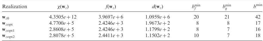
and check closed-loop stability. The process is repeated until there appear closed-loop instability at bf¼bfu. This givesbmin_f ¼bfuþ1. Table 1 lists the values of the FWL stability measure f(wz), the dynamic range measured(wz) and the combined measure(wz) together with the related minimum bit lengthsbmin,bmin_g andbmin_f

for the realizations wz0, wzopt and wzopt1, respectively.

It can be seen that the fixed-point implementation ofwz0

needs at least 42 bits (20 fractional bits and 21 integer bits), while the implementation of wzopt needs at least

17 bits (8 fractional bits and 8 integer bits). The latter achieved a reduction of 25 bits in the required bit length. It can also be seen that, as expected,fðwzopt1Þ ¼fðwzoptÞ

but d(wzopt1) is smaller than d(wzopt), giving rise

to further one bit reduction in bmin

g for wzopt1. Note

that most of the existing FWL design methods, such as the one derived in Li (1998), can at the best hope to attain the realizationwzopt. In fact, the method presented

in Li (1998) may not always be able to achieve this optimal realization, as this method can generally attain a suboptimal solution, see Whidborneet al. (2000b). Thus the advantages of our proposed approach over these existing methods are selfevident.

For a comparison with the direct optimization approach (Wu et al. 2003), the optimization problem (90) was formed, and the MATLAB routine fmin-search.m was used to solve this mm¼16-dimensional search problem. Usingwz0as the initial realization, the

solution obtained by this numerical search was found to be much worst than wzopt. This highlighted a

difficulty with this approach of directly minimizing the combined measure (89). The search space had a much higher dimension and the solution obtained was sensitive to the initial condition. Using wzopt1 as the

initial realization to form (90), the following optimal transformation matrix was obtained

which produced a corresponding optimal realization

wzopt2. The values of various measures and related

minimum bit lengths for wzopt2 are also listed in

table 1. As expected, (wzopt2) <(wzopt1) but f(wzopt2) >f(wzopt1). Although wzopt2 has a smaller

dynamic range than wzopt1, the amount of reduction

is not enough to produce one-bit reduction in bmin

g for wzopt2. Also note that, although f(w) is linked to

bmin

f , the relationship is not a simple one. This is reflected in the result that wzopt2 requires two more

bits in bmin

f , compared with wzopt1. In this case, the

proposed two-procedure approach was able to obtain a better realization wzopt1, in comparison with the

direct optimization approach.

It is obvious that any realization w 2 S

imple-mented in infinite precision will achieve exactly the same set of closed-loop eigenvalues as the infinite-precision implemented w0, which is the designed

closed-loop eigenvalues. For this reason, the infinite-precision implemented wz0 is referred to as the ideal

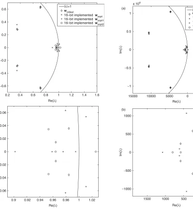
realization wzideal. Figure 2 compares the designed

eigenvalues of the closed-loop system using wzideal

with those of the 16-bit (8 integer bits and 7 fractional bits) implemented wzopt, 16-bit (7 integer

bits and 8 fractional bits) implemented wzopt1, and

16-bit (7 integer bits and 8 fractional bits) imple-mented wzopt2. Confirming the results of table 1,

figure 2 shows that the closed-loop system with the 16-bit implemented wzopt1 is stable while the system

with the 16-bit implemented wzopt or wzopt2 is

unstable.

Similarly, the optimal realization problems in the operator with different values of h were cons-tructed and solved. For example, given h¼214, the

Tzopt2¼

3:3536eþ2 7:5296eþ3 1:4101eþ3 4:7942eþ3 3:4834eþ2 6:7222eþ3 8:1255eþ2 4:0422eþ3 7:9174eþ2 6:0888eþ3 2:5691eþ3 3:5754eþ3 1:0231eþ3 5:5884eþ3 3:9358eþ3 3:3879eþ3

2 6 6 6 4

3 7 7 7 5

Table 1. Comparison of various controller realizations usingzoperator.

Realization (wz) f(wz) d(wz) bminf bming b

min

wz0 4.3505eþ12 3.9697eþ6 1.0959eþ6 20 21 42

wzopt 4.7700eþ5 2.4246eþ3 1.9673eþ2 8 8 17

wzopt1 2.8608eþ5 2.4246eþ3 1.1799eþ2 8 7 16

discrete-time plant model usingoperator was

The controller realization wopt¼w(Topt) calculated

by (14) was a global optimal realization in operator that minimized the FWL closed-loop stability measure (21). The optimization problem (88) was next formed, and the MATLAB routine fminsearch.m yielded the solution

1opt¼8:0159e1, 2opt¼2:9926eþ0,

3opt¼ 5:5715e2,

4opt¼2:8273eþ0, 5opt¼ 9:7594e1,

6opt¼ 6:8654e2:

The global optimal realization with the smallest dynamic range, wopt1¼wopt(Vopt), was readily calculated

according to (84) and (68). The optimization problem (90) was also formed using wopt1 as the initial

realization, and the MATLAB routine fminsearch.m

produced the solution

which yielded the corresponding optimal

realizationwopt2.

Table 2 compares the values of various measures and related minimum bit lengths for the four controller realizations w0, wopt, wopt1 and wopt2 with h¼214.

Note that for the operator with sufficiently small

h, bmin

f can be negative. This simply means that the roundoff is allowed to occur into the integer part of fixed-point representation, and the perturbation error

k"kM, defined in (20), can be larger than 1. In this case, the minimum bit length bmin_¼bmin

g þbminf þ1 required for fixed-point representation can be smaller than bmin_g

that defines the dynamic range of the representation. As an example, ‘‘4 fractional bits’’ means that the entire fractional part and the first lowest 4-bit integer part

A¼

4:4492eþ4 8:8708eþ4 5:9843eþ4 1:5797eþ4

1:6384eþ4 1:6384eþ4 0 0

0 1:6384eþ4 1:6384eþ4 0

0 0 1:6384eþ4 1:6384eþ4

2 6 6 6 4

3 7 7 7 5,

B¼ 1:6384eþ4 0 0 0

T

,

C¼ 1:1160e6 4:3000e8 1:0880e6 1:4000e8

:

The initial realization of the digital controller using theoperator withh¼214 was

F0¼

2:7432eþ4 9:4119eþ4 4:1126eþ4 1:5038eþ4 4:7135eþ3 1:6834eþ4 1:1378eþ4 1:4640eþ2

5:5333eþ3 1:6171eþ4 2:1778eþ4 6:9414eþ1

1:3602eþ3 5:2410eþ1 1:5058eþ4 1:6401eþ4

2 6 6 6 4

3 7 7 7 5,

G0¼ 1:7956eþ10 1:0457eþ10 4:9582eþ9 1:2188eþ9

T

,

J0¼ 1:8180e1 2:8313e1 5:0006e2 6:1722e2

,

M0¼0, H0¼ 0 0 0 0

T

:

The procedure ofx3 was applied, which obtained

Topt¼

5:1914eþ4 8:8698eþ5 5:7412eþ3 7:4766eþ5

8:5895eþ4 9:0040eþ5 1:1049eþ5 4:4017eþ5

1:2078eþ5 9:1282eþ5 2:0407eþ5 2:1153eþ5

1:5654eþ5 9:2419eþ5 2:9242eþ5 5:2325eþ4

2 6 6 6 4

3 7 7 7 5:

Topt2¼

5:7439eþ5 7:7021eþ5 2:9197eþ5 5:9710eþ5 5:5729eþ5 6:8978eþ5 3:9745eþ4 4:6427eþ5 5:3563eþ5 6:3592eþ5 2:9971eþ5 3:7509eþ5 5:0873eþ5 6:0416eþ5 5:0002eþ5 3:2746eþ5

2 6 6 4

in fixed-point representation are omitted. From table 2, it can be seen that the fixed-point implementation ofw0

needs at least 51 bits (15 fractional bits and 35 integer bits) while the implementation ofwoptrequires at least

13 bits (4 fractional bits and 16 integer bits). It can also be seen thatwopt1 and wopt2 give further one bit

reduction inbmin

g , compared withwopt. In this case, the

two different realizationwopt1andwopt2seem to have

15000 10000 5000 0 5000

−1

−0.5 0 0.5 1

x 104

Re(λ)

Im(

λ

)

|λ+214|=214

w_δideal

12–bit implemented w_δopt 12–bit implemented w_δopt1 12–bit implemented w_δopt2 (a)

1500 1000 500 0 500

−1000

−500 0 500 1000

Re(λ)

Im(

λ

)

(b)

Figure 3. Closed-loop eigenvalues of wideal, 12-bit

implemented wopt, 12-bit implemented wopt1 and 12-bit

implementedwopt2, givenh¼214: (a) full plot (b) part of plot. 0.2 0.4 0.6 0.8 1 1.2 1.4 1.6

−0.6

−0.4

−0.2 0 0.2 0.4 0.6

Re(λ)

Im(

λ

)

|λ|=1

w_zideal

16–bit implemented w_zopt 16–bit implemented wzopt1 16–bit implemented wzopt2 (a)

0.9 0.92 0.94 0.96 0.98 1 1.02

−0.06

−0.04

−0.02 0 0.02 0.04 0.06

Re(λ)

Im(

λ

)

(b)

Figure 2. Closed-loop eigenvalues of wzideal, 16-bit

implemented wzopt, 16-bit implemented wzopt1 and 16-bit

implementedwzopt2: (a) full plot (b) part of plot.

Table 2. Comparison of various controller realizations usingoperator withh¼214.

Realization (w) f(w) d(w) bmin_f bming b

min

w0 4.9759eþ15 2.7712eþ5 1.7956eþ10 15 35 51

wopt 1.7287eþ4 3.3740e1 5.1236eþ4 4 16 13

wopt1 8.7084eþ3 3.3740e1 2.5810eþ4 4 15 12

similar robustness to the FWL error. Figure 3 compares the closed-loop eigenvalues of wideal, the

infinite-precision implemented w0, with those of the 12-bit

(5 fractional bits and 16 integer bits) implemented

wopt, the 12-bit (4 fractional bits and 15 integer bits)

implemented wopt1 and the 12-bit (4 fractional bits

and 15 integer bits) implementedwopt2. As expected, the

closed-loop system with the 12-bit implemented wopt1

orwopt2 is stable, but the closed-loop system with the

12-bit implementedwopt is unstable.

Table 3 compares the values of the FWL stability measure f(wopt1) and the dynamic range measure d(wopt1) together with the related minimum bit lengths

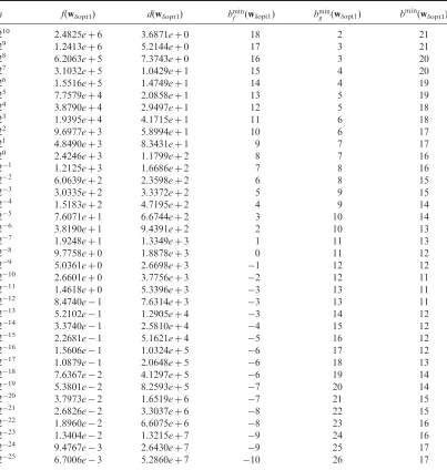
for the controller realizationwopt1, givingh¼210 225.

Comparing tables 1 and 3, it is seen thatwzopt1andwopt1

ofh¼20¼1 have the identical FWL closed-loop stability characteristics, as is expected according to the definition (6). In general, as h decreases, f(wopt1) and hence bmin

f ðwopt1Þ decrease, while d(wopt1) and bming ðwopt1Þ

increase. Before certain values of h (in this case, 210

, 211, 212), the reduction inbmin_f outpaces the increase in

bmin

g and, as a consequence,b

min

decreases ashdecreases. However, whenhis smaller than these values, the increase inbmin_g outpaces the decrease inbmin_f and, consequently,

bmin increases as h decreases. It can be concluded that there exist optimal values of h for the operator and the resulting optimal controller realizations wopt1

achieve the maximum robustness to the FWL errors. Table 3. Comparison ofwopt1under differenth.

h f(wopt1) d(wopt1) bminf ðwopt1Þ bming ðwopt1Þ bmin(wopt1)

210 2.4825eþ6 3.6871eþ0 18 2 21

29 _{1.2413eþ6 5.2144eþ0 17 3 21}

28 6.2063eþ5 7.3743eþ0 16 3 20

27 _{3.1032eþ5 1.0429eþ1 15 4 20}

26 1.5516eþ5 1.4749eþ1 14 4 19

25 7.7579eþ4 2.0858eþ1 13 5 19

24 3.8790eþ4 2.9497eþ1 12 5 18

23 1.9395eþ4 4.1715eþ1 11 6 18

22 _9.6977

eþ3 5.8994eþ1 10 6 17

21 4.8490eþ3 8.3431eþ1 9 7 17

20 _{2.4246eþ3 1.1799eþ2 8 7 16}

21 1.2125eþ3 1.6686eþ2 7 8 16

22 6.0639eþ2 2.3598eþ2 6 8 15

23 3.0335eþ2 3.3372eþ2 5 9 15

24 1.5183eþ2 4.7195eþ2 4 9 14

25 7.6071eþ1 6.6744eþ2 3 10 14

26 3.8190eþ1 9.4391eþ2 2 10 13

27 _{1.9248eþ1 1.3349eþ3 1 11 13}

28 9.7758eþ0 1.8878eþ3 0 11 12

29 _{5.0361eþ0 2.6698eþ3 1 12 12}

210 2.6601eþ0 3.7756eþ3 2 12 11

211 1.4618eþ0 5.3396eþ3 3 13 11

212 8.4740e1 7.6314eþ3 3 13 11

213 5.2102e1 1.2905eþ4 3 14 12

214 _3.3740

e1 2.5810eþ4 4 15 12

215 2.2681e1 5.1621eþ4 5 16 12

216 _{1.5606e1 1.0324eþ5 6 17 12}

217 1.0879e1 2.0648eþ5 6 18 13

218 7.6367e2 4.1297eþ5 6 19 14

219 5.3801e2 8.2593eþ5 7 20 14

220 3.7973e2 1.6519eþ6 7 21 15

221 2.6826e2 3.3037eþ6 8 22 15

222 1.8960e2 6.6075eþ6 8 23 16

223 _{1.3404e2 1.3215eþ7 9 24 16}

224 9.4767e3 2.6430eþ7 9 25 17

6. Conclusions

A novel two-procedure approach has been developed to design optimal fixed-point realizations of digital controllers with FWL considerations. The proposed strategy first finds an optimal controller realization by minimizing an FWL closed-loop stability measure. The fixed-point implementation of this realization thus requires a minimum fractional bit length to guarantee closed-loop stability. This realization is then modified via an effective numerical optimization to produce an optimal realization with the smallest dynamic range without sacrificing FWL closed-loop stability robust-ness. The final optimal realization thus also requires a minimum integer bit length to avoid overflow and consequently it needs a minimum total bit length in fixed-point implementation. Our approach has been developed within the unified framework that includes both the shift and delta operator parameterizations of a generic controller structure. A design example has demonstrated that the proposed method provides an effective design procedure for obtaining optimal controller realizations that are robust to the FWL errors in fixed-point implementation. Simulation results have shown that, by choosing the value ofhin the delta operator appropriately, the optimal delta-operator controller realization has much better FWL closed-loop stability characteristics than the optimal shift-operator controller realization.

Acknowledgements

J. Wu and J. Chu wish to thank the support of the National Natural Science Foundation of China (Grants No. 60374002 and No. 60421002), 973 program of China (Grant No. 2002CB312200) and program for New Century Excellent Talents in University (NCET-04-0547). S. Chen wish to thank the support of the United Kingdom Royal Academy of Engineering.

References

S. Chen, J. Wu, R.S.H. Istepanian and J. Chu, ‘‘Optimizing stability bounds of finite-precision PID controller structures’’,IEEE Trans. Automatic Control, 44, pp. 2149–2153, 1999.

S. Chen, R.S.H. Istepanian, J. Wu and J. Chu, ‘‘Comparative study on optimizing closed-loop stability bounds of finite-precision controller structures with shift and delta operators’’, Systems and Control Letters, 40, pp. 153–163, 2000.

S. Chen, J. Wu and G. Li, ‘‘Two approaches based on pole sensitivity and stability radius measures for finite precision digital controller realizations’’,Systems and Control Letters, 45, pp. 321–329, 2002. M.A. Dahleh and I.J. Diaz-Bobillo, Control of Uncertain

Systems: A linear Programming Approach, Englewood Cliffs, NJ: Prentice Hall, 1995.

J.-P. Delmas, ‘‘Performances analysis of a Givens parameterized adaptive eigenspace algorithm’’,Signal Processing, 68, pp. 87–105, 1998.

M.C. De Oliveira and R.E. Skelton, ‘‘State feedback control of linear systems in the presence of devices with finite signal-to-noise ratio’’, Int. J. Control, 74, pp. 1501–1509, 2001.

I.J. Fialho and T.T. Georgiou, ‘‘On stability and performance of sampled-data systems subject to wordlength constraints’’, IEEE Trans. Automatic Control, 39, pp. 2476–2481, 1994.

I.J. Fialho and T.T. Georgiou, ‘‘Computational algorithms for sparse optimal digital controller realizations’’, in Digital Controller Implementation and Fragility: A modern Perspective, R.S.H. Istepanian and J.F. Whidborne, Eds., London: Springer Verlag, 2001, pp. 105–121.

M. Gevers and G. Li, Parameterizations in Control, Estimation and Filtering Problems: Accuracy Aspects, London: Springer Verlag, 1993.

R.S.H. Istepanian and J.F. Whidborne (Eds.) Digital Controller Implementation and Fragility: A Modern Perspective, London: Springer Verlag, 2001.

T. Kailath,Linear Systems, Upper Saddle River, NJ: Prentice Hall, 1980.

L.H. Keel and S.P. Bhattacharryya, ‘‘Robust, fragile, or optimal?’’, IEEE Trans. Automatic Control, 42, pp. 1098–1105, 1997. G. Li, ‘‘On the structure of digital controllers with finite word length

consideration’’,IEEE Trans. Automatic Control, 43, pp. 689–693, 1998.

K. Liu, R.E. Skelton and K. Grigoriadis, ‘‘Optimal controllers for finite wordlength implementation’’,IEEE Trans. Automatic Control, 37, pp. 294–1304, 1992.

P. Mantey, ‘‘Eigenvalue sensitivity and state-variable selection’’,IEEE Trans. Automatic Control, 13, pp. 263–269, 1968.

R.H. Middleton and G.C. Goodwin,Digital Control and Estimation: A Unified Approach, Englewood Cliffs, NJ: Prentice Hall, 1990. J. O’Reilly,Observers for Linear Systems, New York: Academic Press,

1983.

G. Owen,Game Theory, New York: Academic Press, 1982.

V. Pareto,Manuale di Economia politica, Milan, Italy: Societa Editrice Libraria, 1906.

J. Sze´p and F. Forgo´,Introduction to the Theory of Games, Dordrecht, Holland: D. Reidel Publishing Company, 1985.

J.F. Whidborne, J. Wu and R.S.H. Istepanian, ‘‘Finite word length stability issues in an l1 framework’’, 73, pp. 166–176, 2000a. J.F. Whidborne, J. Wu, R.S.H. Istepanian and J. Chu, ‘‘Comments on

On the structure of digital controllers with finite word length consideration’’,IEEE Trans. Automatic Control, 45, pp. 344–344, 2000b.

J.F. Whidborne, R.S.H. Istepanian and J. Wu, ‘‘Reduction of controller fragility by pole sensitivity minimization’’,IEEE Trans. Automatic Control, 46, pp. 320–325, 2001.

J. Wu, S. Chen, G. Li, R.S.H. Istepanian and J. Chu, ‘‘Shift and delta operator realizations for digital controllers with finite-word-length considerations’’, IEE Proc. Control Theory and Applications, 147, pp. 664–672, 2000.

J. Wu, S. Chen, G. Li, R.S.H. Istepanian and J. Chu, ‘‘An improved closed-loop stability related measure for finite-precision digital controller realizations’’, IEEE Trans. Automatic Control, 46, pp. 1162–1166, 2001.

J. Wu, S. Chen, G. Li and J. Chu, ‘‘Global optimal realizations of finite precision digital controllers’’, inProc. 41st IEEE Conf. Decision and Control, Las Vegas, USA, Dec. 10–13, pp. 2941–2946, 2002. J. Wu, S. Chen, J.F. Whidborne and J. Chu, ‘‘A unified close-loop

stability measure for finite-precision digital controller realizations implemented in different representation schemes’’, IEEE Trans. Automatic Control, 48, pp. 816–822, 2003.

J. Wu, S. Chen, G. Li and J. Chu, ‘‘A search algorithm for a class of optimal finite-precision controller realization problems with saddle points’’,SIAM J. Control and Optimization, 44, pp. 1787–1810, 2005. K. Zhou, J.C. Doyle and K. Glover, Robust Optimal Control,

Englewood Cliffs, NJ: Prentice Hall, 1996.