Correcting for misclassification error in gross flows using double sampling: moment based inference vs likelihood based inference

Correcting for Misclassification Error in Gross Flows Using Double

Sampling: Moment-based Inference vs. Likelihood-based Inference

Nikos Tzavidis

Abstract

Gross flows are discrete longitudinal data that are defined as transition counts, between a finite number of states, from one point in time to another. We discuss the analysis of gross flows in the presence of misclassification error via double sampling methods. Traditionally, adjusted for misclassification error estimates are obtained using a moment-based estimator. We propose a likelihood-based approach that works by simultaneously modeling the true transition process and the misclassification error process within the context of a missing data problem. Monte-Carlo simulation results indicate that the maximumlikelihood estimator is more efficient than the moment-based estimator.

Correcting for Misclassification Error in Gross Flows Using Double Sampling:

Moment-based Inference vs. Likelihood-based Inference

Nikos Tzavidis1 Abstract

Gross flows are discrete panel data that are generally defined as transition counts, between a finite number of states, from one point in time to another. Gross flows are typically estimated by linking panel data from consecutive waves. This process, however, is affected by the existence of non-sampling errors such as response errors that cause misclassification error. We discuss alternative approaches for correcting for misclassification error in gross flows via double sampling. Traditionally, in a double sampling context, adjusted for misclassification error estimates are obtained using a moment-based estimator. We propose a likelihood-based approach that works by simultaneously modeling the true transition process and the misclassification error process within the context of a missing data problem. The model is formulated under alternative double sampling designs and maximum likelihood estimates are derived by maximizing the likelihood of the augmented data via the EM algorithm. The issue of variance estimation for the adjusted estimates is resolved using Taylor series linearization and the Missing Information Principle. Monte-Carlo simulation results indicate that the maximum likelihood estimator is more efficient than the moment-based estimator while a real data application indicates that the maximum likelihood estimator has desirable numerical properties that are appealing to the data analyst.

KEYWORDS: Nonsampling errors; Response bias; Panel surveys; Re-interview surveys; Missing data; Labour force gross flows

1. Introduction

Gross flows are defined as transition counts, between a finite number of states, from one point in time to another. Typical examples of gross flows are labour force gross flows that represent transition counts of the labour force population between the different labour force states. Gross flows estimates are frequently derived from panel surveys by linking panel data from consecutive

1

waves. This process, however, is affected by non-sampling errors such as response errors that cause misclassification error (Hogue and Flaim 1986; Kristiansson 1999).

The existence of misclassification error in data used for statistical analysis can introduce serious bias in the derived results. Methods that account for the existence of misclassification error have received great attention in the statistical literature. In the presence of misclassification error, such methods need to be employed in order to ensure the validity of the inferential process. One of the traditional approaches for adjusting for misclassification error in discrete data, such as gross flows, is by assuming the existence of validation information derived from a validation survey, which is free of error. The use of validation surveys can be placed into the framework of double sampling methods (Bross 1954). In a double sampling framework we assume that along with the main measurement device, which is affected by misclassification error, we have a secondary measurement device (validation survey), which is free of error but more expensive to apply. Due to its higher cost, the validation survey is employed only for a subset of sampling units. Inference using double sampling is based on combining information from both measurement devices. Other approaches to misclassification error correction include latent class models (Van de Pol and De Leeuw 1986) and instrumental variables models (Skinner and Humphreys 1997). However, in this paper, we will focus on the case that validation data, obtained via double sampling, are available.

We examine alternative approaches for correcting for misclassification error in gross flows when validation information is available. However, while the main measurement device is a panel survey, we allow only for cross-sectional validation data. This choice can be justified given the costs associated with conducting a validation survey. We propose a maximum likelihood estimator as an alternative to the traditional moment-based estimator. We show that in contrast to the moment-based estimator, the maximum likelihood estimator provides more efficient adjusted estimates and has numerical properties that are appealing to the data analyst.

with panel data along with alternative specifications for quantifying the misclassification error mechanism. In Section 3 we describe two alternative approaches for misclassification error correction via double sampling. The first approach is an existing one that leads to a moment-based estimator. The second approach is what we propose and leads to a maximum likelihood estimator. Both approaches are investigated under alternative double sampling designs. In Section 4 we discuss variance estimation for the moment-based and the maximum likelihood estimators. In Section 5 a series of Monte-Carlo simulation studies are designed for empirically comparing the alternative point and variance estimators while in Section 6 the methodology is illustrated in the context of the US Current Population Survey (CPS) by estimating labour force gross flows adjusted for misclassification error. Finally, in Section 7 we summarize the main findings and provide directions for further research.

2. Using Double Sampling for Misclassification Error Correction

Suppose that the standard measurement device is subject to misclassification error. As a result we have biased results. Unbiased estimates can be obtained by utilizing more elaborate measurement tools usually referred to as preferred procedures (Forsman and Schreiner 1991; Kuha and Skinner 1997). An example of a preferred procedure is re-interview surveys (Bailar 1968). In bio-statistical applications the term “gold standard” is more commonly used (Bauman and Koch 1983). Other examples include judgments of experts or checks against administrative records (Greenland 1988). The assumption that the preferred procedure is free of error makes possible the estimation of the parameters of the misclassification error mechanism. On the other hand, the preferred procedures are considered to be fairly expensive and thus unsuitable to be used for the entire sample. Therefore, these procedures are normally applied to a smaller sample usually referred to as validation sample.

validation sample is whether the fallible classifications from the validation sample can be combined with the fallible classifications from the main sample. A validation sample is defined as internal if it is a sub-sample of units from the main sample of n units obtained via a randomised double sampling design. Alternatively, the validation sample is defined as internal if it is selected independently from the main sample and from the same target population. Otherwise, the validation sample is characterised as external. The parameters of the misclassification error mechanism estimated from an external validation sample are assumed to be representative of the misclassification process in the target population but the fallible classifications from this validation sample cannot be combined with the fallible classifications from the main sample.

v n

Initially, double sampling methods were developed to adjust cross-sectional data for misclassification error. In this context, Bross (1954) described the general framework of double sampling methods. Maximum likelihood adjusted estimates for binomial and multinomial data were derived by Tenenbein (1970;1972) respectively. These results were then extended for fitting log-linear models in the presence of misclassification error (Espeland and Odoroff 1985). It is believed that for cross-sectional data there is no particular tendency for errors to be systematic (Skinner 2000). However, for panel data produced by linking information on the same individual in different time points, this cancellation may not occur. Work on the adjustment of gross flows for misclassification error via the use of double sampling includes Abowd and Zellner (1985), Poterba and Summers (1986), Skinner and Torelli (1993), and Singh and Rao (1995).

2.1 Double Sampling Designs for Panel Data Analysis

In this section we examine three alternative double sampling designs that can be used with panel misclassified data when only cross-sectional validation data are available.

Double Sampling Design 1

A simple random sample of n units is selected from a population of N units and the classifications for these n units are obtained at time t and using a standard measurement device, which is affected by misclassification error. At a second time point, between t and ,

1 +

t

1 +

a sub-sample of units is selected from the n units that already belong to the main sample and their classifications by the standard measurement device at time t are validated using more elaborate survey techniques.

v n

Double Sampling Design 2

A simple random sample of n units is selected from a population of N units and the classifications for these n units are obtained at time t and using the standard measurement device, which is affected by misclassification error. For another simple random sample of units, independently selected from the main sample and from the same target population, classifications are obtained only at time t using also the standard measurement device. At a second time point, between t and , the classifications of the units obtained by the standard measurement device are validated using more elaborate survey techniques.

1 +

t

v n

1 +

t _nv

Double Sampling Design 3

A simple random sample of n units is selected from a population of N units and the classifications for these n units are obtained at time t and using a standard measurement device, which is affected by misclassification error. Using an external source of information, we then obtain cross-sectional information on the incidence of error. The assumption underpinning this design is that the external source of information adequately describes the misclassification process in the target population.

1 +

t

sampling designs. The different double sampling designs have also different costs. Under design 2 we conduct the main survey using n units and the validation survey using different units. Therefore, under this design we have cross-sectional information on the observed classifications for units. On the other hand, under design 1 we have cross-sectional information on the observed classifications only for n units. This implies that design 2 may be associated with an increased cost compared to design 1. In this discussion, however, we need to consider one of the main disadvantages associated with design 1. Under this design, the sample units that participate in the validation survey participate also in the main, panel, survey. One may argue that this is similar to adding an extra wave to the panel survey, which effectively may increase the response burden of the respondents and therefore impact on the quality of the collected data.

v n

+ v

n n

2.2 Quantifying the Misclassification Error Mechanism

Assume that a sample of n units has been selected via a randomised design from a population of units and let ξ denote a member of this sample. Let us further assume that the variable of interest, measured by the survey, is subject to misclassification error and that a validation survey is used for identifying the true values for a subset of sample units. Define the random variables , that respectively describe the observed and true classifications for the sample unit at time . One way to quantify the misclassification error mechanism is via the use of misclassification probabilities defined as (see for example Tenenbein 1972). An alternative approach is by using what Carroll (1992) refers to as calibration probabilities. The calibration probabilities are defined as .

N

∗ ξt Y Y_ξt

th ξ

t

Pr( ∗ | )

ξ ξ

= = =

ik t t

q Y i Y k

i

(

)

Pr | ∗

ξ ξ

= = =

ki t t

c Y k Y

probabilities, calibration probabilities can be used only with internal validation samples. This is because calibration probabilities condition on the observed classifications, which can not be considered as transportable to the population of interest when only external validation data exist. Nevertheless, here we argue that an external validation sample can be transformed into an internal validation sample. Since the misclassification process in the external validation sample is assumed to be representative of the misclassification process in the target population, we propose to calibrate Pr

(

Y_ξ∗_t =i Y, _ξt =k

)

on the marginal information derived from the main sample. In the simplest case, this calibration procedure can be performed using an Iterative Proportional Fitting (IPF) algorithm (Deming and Stephan 1940). This transformation will be assumed throughout this paper when employing double sampling design 3.

In a cross-sectional context Tenenbein (1970,1972) developed maximum likelihood estimators using calibration probabilities. In a recent paper, Tzavidis and Lin (2004) proposed a missing data specification that utilises misclassification probabilities for deriving maximum likelihood or quasi-likelihood estimates. All previous approaches lead to identical results.

argues that the main difference between the use of misclassification or calibration probabilities is in assumption (b) and concludes that the use of the ICE assumption with misclassification probabilities is more reasonable. Therefore, in this paper we will consider only misclassification probabilities.

3. Two Alternative Specifications for Misclassification Error Correction via Double Sampling

In this section we present two alternative specifications for adjusting for misclassification error in gross flows. The first one leads to a moment-based estimator that has been already proposed in the literature (Poterba and Summers 1986; Singh and Rao 1995). The second specification is what we propose and is based on expressing the misclassification problem as a missing data problem, which we solve via the EM algorithm (Dempster; Laird and Rubin 1976). This second approach leads to maximum likelihood estimates.

3.1 Moment-based Inference for Gross Flows under Misclassification Error and Double Sampling

Suppose that we conduct a panel survey where a sample unit ξ is interviewed at two consecutive time points . The variable of interest, i.e. the flows between r mutually exclusive states measured by the panel survey, is subject to misclassification error. Denote by the probability that unit truly belongs in state k at t and state l at and by the probability that unit is observed in state i at t and state at . Let P denote the matrix with elements and Π the matrix with elements . Corresponding to each element of Π and unit we define the random variables , , which describe the observed (affected by misclassification error) classifications of unit at t and . We also define the random variables , which describe the true classifications of unit ξ at t and . The pairs

, +

t t 1

+

kl P

ξ t+1 Π_ij

ξ j t +1

kl

P Πij

ξ ∗

ξt

Y 1

∗ ξt Y

ξ t +1

1

, ξt ξt+

Y Y t +1

(

, 1

)

∗ ∗

ξt ξt+

misclassification error process. The misclassification probabilities are denoted by and the matrix of misclassification probabilities

by .

1

Pr( ∗ |∗ )

ξ ξ+ ξ ξ+

= = = =

ijkl t t t t

q Y i Y j Y k Y 1 =l

)

1=l

)

.

)

)

)

)

)

1

( , +1)

Q t t

Generally speaking, the misclassification error model is defined by expressing the joint distribution of the observed and true classifications as a product of the misclassification probabilities times the true transition probabilities as follows

(3.1)

(

1

)

1 1

(

1 1

Pr ∗ ∗ Pr( ∗ ∗ | ) Pr

ξ ξ+ ξ ξ+ ξ ξ+ ξ ξ+

= =

= = =

∑∑

r r = = = = =

t t t t t t t t

k l

Y i Y j Y i Y j Y k Y l Y k Y

Expressing (3.1) in vector notation, assuming that is non-singular and solving the resulting system of equations with respect to the vector of true flows P we obtain the following expression for the adjusted gross flows

( , +1

Q t t

vec P( )=

[

Q t t(, +1)

]

−1vec( )Π (3.2) The estimation of the misclassification matrix is not straightforward. To see this note that the number of free parameters when estimating is equal to . This implies that information obtained from a cross-sectional validation sample is not sufficient to determine . We therefore need to introduce additional assumptions that will enable us to estimate the longitudinal misclassification matrix. The assumption that we utilise is the ICE one with misclassification probabilities (Section 2.2), which is more rigorously defined as follows:

(, +1

Q t t

( , +1

Q t t _{r r}2

(

2 ₋₁

( , +1

Q t t

Pr

(

Y_ξ∗_t =i Y, _ξ∗_t+1 = j Y| _ξt =k Y, _ξt+1 = =l

)

Pr

(

Y_ξ∗_t =i Y| _ξt =k

) (

PrY_ξ∗_t+1 = j Y| _ξt+ =l . Restating the ICE assumption we can say that (a) The observed classifications are conditionally independent given the true classifications and (b) The misclassification at

depends only on the current true state and not on the previous or future true states. Denote by 1

,

∗ ∗

ξt ξt+ Y Y

1

, ξt ξt+ Y Y

t

( )

Q t the cross-sectional matrix of misclassification probabilities at time t with elements , by the cross-sectional matrix of misclassification probabilities at with elements

ik q

( +1

and by the kronecker product. An implication of ICE is that the longitudinal misclassification matrix can now be expressed in matrix notation as follows:

⊗

Q t t(, +1)=Q t( +1)⊗Q t( ) .

)

However, since Q t( +1 is not known, we further assume that Q t( )=Q t( +1)(assumption of stationary misclassification error). Assuming now that all quantities involved in the measurement error model can be estimated by utilising a double sampling design and the ICE assumption, an estimator of (3.2) is given by the following expression

( )

( ) ( )

( )

1

. −

∧ _⎡∧ ∧ _⎤ ∧

= _⎢ ⊗ _⎥

⎣ ⎦

vec P Q t Q t vec Π (3.3) Let us now examine the effect of the choice of double sampling design on the moment-based estimator. Since we allow only for cross-sectional validation data, the validation sample is used for estimating the parameters of the misclassification error mechanism while the main sample is used for estimating gross flows. This is true under all three double sampling designs. Thus, the choice of double sampling design has no effect on point estimation performed via the moment-based estimator. Differences may be encountered in variance estimation due to the extra covariance terms introduced under double sampling design 1. This is investigated in Section 4.

A drawback associated with the use of the moment-based estimator is that under certain conditions it can produce estimates that lie outside the parameter space. This can happen due to the inversion of the misclassification matrix involved in (3.3). As an alternative to the moment-based estimator, in the upcoming section we propose a maximum likelihood estimator.

3.2 Likelihood-based Inference for Gross Flows under Misclassification Error and Double Sampling

are considered. In Section 3.2.1 we allow for double sampling design 2 while in Section 3.2.2 we allow for double sampling design 1. The case of double sampling design 3 is covered by double sampling design 2 using the transformation described in Section 2.2.

3.2.1 Likelihood-based Inference under Double Sampling Design 2

Let us assume that the panel survey that is utilized for estimating gross flows is affected by misclassification error and that a cross-sectional validation sample of units is selected via double sampling design 2. The main survey provides information about the flows of the sample units between mutually exclusive states at t and . On the other hand, the validation survey provides information about the cross-sectional incidence of misclassification error related to these states at t. In what follows we define a category as a pair of states for which there is a flow, so there are such flow categories.

v n

r t+1

2

r

Consider the cross-classification of the fallible with the true classifications. Denote by

the number of sample units classified in cell ij defined by this cross-classification in the main and in the validation samples respectively. We formulate a model by combining information from both samples. This will eventually lead to a missing data problem. One source of missing data is attributed to the different time dimensions of the main and the validation surveys. The other source of missing data is due to the fact that individuals participating in the main survey do not participate in the validation survey.

, v ij ij n n

Denote by the probability that a respondent truly belongs in category i and by the probability that a respondent is classified in category given that he/she truly belongs in category

. The probability that a sample unit belongs in cell ij is expressed as a product of the true transition probabilities and the misclassification probabilities. Denote further by Θ the vector of parameters, by the complete (augmented) data and by a superscript ( _{any missing data.}

Assuming independence between the main and the validation samples, the likelihood function of the augmented data is given by

i

P qij

j i

Complete

(

)

(

)

( )

(

)

( )

2 2 2 2

1 1 1 1

; ∗ ∗.

= = = =

Θ _Complete =

∏∏

r r nij

∏∏

r r ijv

i ij i ij

i j i j

L D Pq Pq n

Taking the logarithms on both sides and imposing the constraint

2

1

1

=

=

∑

r i i

P

we obtain the following expression for the log-likelihood function of the augmented data

(

)

(

( ) ( )

)

(

( ) ( )

)

(

( ) ( )

) ( )

2 2 2 2

2 2

1 1

1 1 1 1

; − ∗ ∗ log ∗ ∗ log 1 − ∗ ∗ log .

= = = =

⎛ _⎞⎟

⎜ _⎟

Θ = + + + ⎜_⎜ − _⎟⎟+ +

⎜⎝ ⎠

∑

i i i i

∑

∑∑

r r r r

Complete v v v

i i i r r i ij ij ij

i i i j

l D n n P n n P n n q (3.4)

The longitudinal misclassification probabilities, , are unknown and are estimated using the cross-sectional misclassification probabilities and the ICE assumption. The log-likelihood function given in (3.4) is presented in its generic form i.e. without incorporating the ICE assumption. However, after incorporating ICE we need to add the extra constraint that the sum of the cross-sectional misclassification probabilities for a given true classification must add up to one. This extra constraint implies that we have to estimate parameters that describe the misclassification error process and gross flows specific parameters.

ij q

2 ₋

r r

2 ₋₁

r

Since the likelihood function involves missing data, one way of using this likelihood to maximise the likelihood of the observed data is via the EM algorithm. In the sequel we describe the expectation step (E-step) and the maximization step (M-step). Denote by the observed data from the validation sample, by the observed data from the main sample and by

v D m

D ( )h the

current iteration of the EM algorithm. In order to perform the E-step we need to estimate the conditional expectations of the unobserved quantities in the main sample and in the validation sample given the observed data. This can be done using the following result.

Result 3.1

(

( ) ) ( ) ( ) ( ) ( ) 2 1 | , ∧ ∧ ∧ ∗ ∧ ∧ = ⎛ _⎞⎟ ⎜ _⎟ ⎜ _⎟ ⎜ _⎟ ⎜ _⎟ ⎜

Θ = _⎜ ⎟_⎟

⎜ _⎟⎟ ⎜ _⎟ ⎜ _⎟ ⎜ ⎟ ⎝

∑

⎠ i h h i ij m

ij j _{r h}

h i ij i

q P

E n D n

q P

.

Proof

Proof of Result 3.1 is given in Appendix A Result 3.2

Denote by the total number of sample units in the validation sample that belong to the k th cell of the misclassification matrix. The conditional expectations of the missing data in the validation sample are estimated using the following expression

v k n

(

( ) ) ( ) ( ) ( ) ( ) | , ∧ ∧ ∧ ∗ ∧ ∧ ⎛ _⎞⎟ ⎜ _⎟ ⎜ _⎟ ⎜ _⎟ ⎜ _⎟

Θ = ⎜_⎜ ⎟_⎟

⎜ _⎟⎟ ⎜ _⎟ ⎜ _⎟ ⎜⎝

∑∑

⎠ h h i ij

v v v

ij k _h h

i ij i j

q P

E n D n

q P

Proof

Proof of Result 3.2 is given in Appendix A

Having performed the E-step, the missing data in log-likelihood function (3.4) are replaced by the estimated conditional expectations. The M-step can then be performed by numerically maximising (Dennis and Schnabel 1983) the log-likelihood function of the augmented data. The E and M steps are iterated until a convergence criterion, for example the -norm of the vector of parameters derived from two successive iterations of the EM algorithm, is satisfied.

2

L

3.2.2 Likelihood-based Inference under Double Sampling Design 1

− v

n n that participate only in the main survey. On the other hand, the validation survey provides now information on the cross-sectional incidence of misclassification error related to the classifications at time t and on the observed flows of the units that participate both in the main and in the validation surveys. Under this design, the log-likelihood function of the augmented data is also given by (3.4) and is maximized using the EM algorithm. The E-step is described below.

v n

For the main sample the conditional expectations of the missing data can be estimated using Result 3.1. However, for the validation sample estimating the conditional expectations of the missing data cannot be simply based on Result 3.2. This is because under design 1 we need to condition on two sets of observed data (the data from the main sample and the data from the validation sample). Therefore, a two-stage step is employed. For simplicity, we illustrate this E-step for the 4-state model that can be schematically described via a cross-classification of the observed with the true classifications.

4 4×

In the first stage of the E-step we estimate initial conditional expectations using Result 3.2. These provisional conditional expectations will therefore respect the cross-sectional validation information. However, we also need to respect the information about the observed flows of the units in the validation sample. This is achieved at the second stage. Based on the provisional conditional expectations, we compute the following quantities

( ) ( )

( ) ( ) 11 21

13 23

, ,

∗ ∗

∗ ∗

= +

= +

v v

v v

a n n

e n n

( ) ( )

( ) ( ) 12 22

14 24

, ,

∗ ∗

∗ ∗

= +

= +

v v

v v

b n n

f n n

( ) ( )

( ) ( ) 31 41

33 43

, ,

∗ ∗

∗ ∗

= +

= +

v v

v v

c n n

g n n

( ) ( )

( ) ( ) 32 42

34 44 .

∗ ∗

∗

= +

= +

v v

v v

d n n

h n n ∗

}

We then form two 2 tables the margins of which are defined by { }and respectively. It can be easily verified that the margins of these two tables summarise the information available for the units in the validation sample under double sampling design 1. More specifically, the column margins define the observed flows and the row margins define the cross-sectional validation information. Having formed these tables, we then use the IPF (Deming and Stephan 1940) algorithm to rake the internal cells of these matrices to the data constraints that

2

× a b c d, , ,

{e f g h, , ,

we need to respect. The newly derived internal cells are denoted by { }and . It remains to estimate the final conditional expectations of the unobserved quantities in the validation sample. In order to do so we form the 2 vectors that summarise

and { . For example, the 2 vector defined by must respect the constraint that . For the 4-state model one can form 8 such vectors. Using arguments analogous to the ones for Results 3.1 and 3.2, the conditional expectations are then estimated within each of these 2 vectors. For example,

, , , ∗ ∗ ∗ ∗

a b c d

{_{e f g h}∗, , ,∗ ∗ ∗_}

} ∗

∗

1

×

{_{a b c d}∗, , ,∗ ∗ ∗} _{e f g h}∗_{, , ,}∗ ∗ ∗ _×1 ( ) ( ) 11 , 21

∗

v v

n n

( ) ( ) 11 21

∗ ₌ v∗ ₊ v

a n n

1 ×

(

( ) ) ( ) ( ) ( ) ( ) ( )

(

) ( ) ( ) ( ) ( ) 1 2 11 21

11 2 21 2

1 1 1 1 | , , | , ∧ ∧ ∧ ∧ ∧ ∧ ∗ ∗ ∗ ∗ ∧ ∧ ∧ ∧ = = ⎛ ⎞_⎟ ⎛ ⎞_⎟ ⎜ _⎟ ⎜ _⎟ ⎜ _⎟ ⎜ _⎟ ⎜ _⎟ ⎜ _⎟ ⎜ ⎟ ⎜ ⎟

Θ = ⎜_⎜ ⎟_⎟ Θ = ⎜_⎜ ⎟_⎟

⎜ ⎟_⎟ ⎜ ⎟_⎟ ⎜ _⎟ ⎜ _⎟ ⎜ ⎟ ⎜ ⎟ ⎜ ⎜ ⎝

∑

⎠ ⎝

∑

⎠ h h h h

v v v v

h h

h h

i i

i i

i i

q P q P

E n D a E n D a

q P q P

.

These estimated conditional expectations will respect both the cross-sectional validation information and the observed flows of the units in the validation sample. After estimating the conditional expectations of the unobserved quantities in the main and in the validation samples, the M-step is performed numerically.

4. Variance Estimation

Having investigated alternative approaches for point estimation, in this section we develop tools for variance estimation. Variance estimation for the moment-based estimator is discussed in Section 4.1. Variance estimation for the maximum likelihood estimator is discussed in Section 4.2.

4.1 Variance Estimation for the Moment-based Estimator

Using properties of vec operators, the moment-based estimator, under ICE, is given by

( )

1 1 − − ∧ ⎡∧ ∧ ⎛∧ ⎞⎟ ⎤ ⎢ ⎜ ⎥ =_{⎢ ⎜⎜⎝ ⎟⎟⎠ ⎥} ⎣ ⎦

vec P Q Q

Τ

Π (4.1)

In order to simplify the notation, we drop the parenthesis next to Q that is time specific. A variance estimator for (4.1) can be derived by employing the -method (Bishop, Fienberg and Holland 1975). This involves expanding

δ

( )

∧

Let

( )

₁

( ) ( )

, ₂ ,..., 2

( )

∧ ∧ ∧

⎡ ⎤ ₌ ⎡

⎢ ⎥ ⎢

⎣ ⎦ ⎣

T r vec P Θ g Θ g Θ g Θ∧ ⎤_⎥

⎦

)

∧

Π

represent a vector of non-linear functions of a

vector . Recall that denotes the misclassification

probabilities and denotes the observed transition probabilities between t and . Note also that now we distinguish between the subscripts . However, both subscripts refer to the

observed classifications at t. Expanding

2_×1

r

(

₁₁, ₂₁, ₃₁,..., , 11, 21, 31,...,

∧ _{∧ ∧ ∧ ∧} ∧ ∧ ∧

= q q q q_rr rr

Θ Π Π Π q_ik

lj

Π t+1

,

l i

( )

∧

vec P around its true value using Taylor series we

have that

( )

[

( )

]

(

)

,

[

( )

]

| ∧

∧ ∧

=

∂

⎡ ⎤_{− ≈ ∇ − ∇ =}

⎢ ⎥ .

⎣ ⎦

vec

vec P _{Θ Θ}

Θ Θ

Θ

Θ Θ Θ Θ

Θ

∂

P

vec P (4.2)

Taking the variance operator on both sides of (4.2) we have that

{

⎡⎢

( )

∧ ⎤⎥

}

≈ ∇

( )

∧

(

∇

)

.

⎣ ⎦

T

Var vec P Θ ΘVar Θ Θ (4.3)

In order to estimate (4.3), we need to evaluate the Jacobian matrices ∇ ,

(

and estimate

the covariance matrix

Θ ∇

)

T

Θ

( )

∧

Var Θ . For the later case, we need to estimate the following components:

(a) the covariance matrix of the unadjusted estimated probabilities of transition (b) the covariance matrix of the estimated misclassification probabilities and (c) the covariance of

.

∧

lj

Π

∧

ik q

,

∧ _∧

lj q_ik

Π

Under simple random sampling, component (a) can be estimated using standard results for the variance of binomial random variables. Component (b) requires a second application of the -method. This is because the estimated misclassification probabilities are defined as ratios of

random variables. Let . Applying the δ-method to we

derive the following

δ

(

*

11, 21, 31,...,

∧

= v v v v

rr

n n n n

Θ

)

⎡⎢ ⎛ ⎞⎟⎜_{⎜ ⎟⎜}∧* ⎤_⎥⎟

⎢ ⎝ ⎠⎥

⎣ ⎦

( )

( )

* * * * * * * * * * , = | ∧ . ∧ ∧ = ⎡ ⎤ ∂ ⎡ ⎛_⎜ ⎞_⎟⎤ _{⎡ ⎤} ⎛_⎜ ⎞_⎟ ⎢_⎣ ⎥_⎦ ⎢ _{⎜⎜ ⎟}⎟⎥ − _{⎢⎣ ⎥⎦} ≈ ∇ _⎜⎜ − ⎟_⎟ ∇ ⎢ ⎝ ⎠⎥ ⎝ ⎠ ∂ ⎣ ⎦ vec Q

vec Q vec Q _{Θ Θ}

Θ Θ

Θ

Θ Θ Θ Θ

Θ (4.4)

Taking the variance operator on both sides of (4.4) we obtain the following

*

(

)

* * . ∧ ∧ ⎧ ⎫ * ⎡ ⎛ ⎞⎤ ⎛ ⎞ ⎪ ⎪ ⎪ _{⎢ ⎜ ⎟⎥ ≈ ∇}⎪ _{⎜ ⎟ ∇} ⎨ _⎢ ⎜_⎜ ⎟_⎟⎥⎬ ⎜_⎜ ⎟_⎟ ⎪ _⎣ ⎝ ⎠_⎦⎪ ⎝ ⎠ ⎪ ⎪ ⎩ ⎭ T

Var vec Q Θ _ΘVar Θ _Θ (4.5)

In order to estimate (4.5) we need to evaluate the Jacobian matrices ∇_Θ*,

( )

∇ *

T

Θ and the

covariance matrix . Under simple random sampling and taking into account that the

sample size of the validation survey is fixed, we can treat as multinomial counts. Therefore

can be estimated using standard results for the variance of binomial random variables.

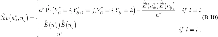
For component (c) i.e. the covariance between the unadjusted estimated probabilities of transition and the estimated misclassification probabilities we distinguish two cases. Under double sampling design 2 and double sampling design 3 we assume that Under double sampling

design 1 we assume that For the latter case we estimate this covariance term using the following result

* ∧ ⎛ _⎟ ⎜ _⎟ ⎜ _⎟ ⎜⎝

Var Θ ⎞

⎠ ⎠ v ik n * ∧ ⎛ _⎞⎟ ⎜ _⎟ ⎜ _⎟ ⎜⎝ Var Θ

(

,

)

0.

∧ ∧

=

lj ik Cov q Π

(

,

)

0.

∧ ∧

≠

lj ik Cov q Π

Result 4.1

An estimator for the covariance term of interest is given by

(

)

( )

( )

( )

₍

₎

( )

( )

* * 1 1 ₁ * * 1 1 1

, Pr , ,

Pr , ,

∧ ∧

∧ ∧

ξ ξ+ ξ

∧

= ₌

∧ ∧

∧

∧

ξ ξ+ ξ

∧ = ⎛ _⎞⎟ ⎜ _{⎟ ⎧⎪} ⎜ _{⎟ ⎪} ⎜ _{⎟ ⎪} ⎜ _{⎟ ≈ ⎨ = = = −} ⎜ ⎟ ⎜ ⎟ ⎛ ⎞⎪ ⎜ ⎟_⎟ ⎜ ⎟⎪ ⎜ _⎟ ⎜ ⎟⎪⎩ ⎜ _{⎜ ⎟⎟} ⎝ ⎠ _{⎝ ⎠} − = = = − ⎛ _⎞⎟ ⎜ _⎟ ⎜ _⎟⎟ ⎜⎝ ⎠

∑

_∑

∑

v v ik lj lj v ik

r _v r t t t v

v ik _ik i _i v v ik lj ik v

t t t

r v ik i

E n E n n

n

Cov n Y i Y j Y k

n n

n _{n E n}

E n E n E n

n Y i Y j Y k

n E n

( )

( )

. ∧ ∧ ≠ ⎫⎪⎪ ⎡ _⎤⎪⎪ ⎢ _{− ⎥⎪} ⎢ _⎥⎬⎪ ⎢ _⎥⎪ ⎢ ⎥⎪ ⎣ _⎦⎪ ⎪⎭

∑

ikv lj

v v

l i

E n E n n

Proof

4.2 Variance Estimation for the Maximum Likelihood Estimator

In this section we perform variance estimation for the maximum likelihood estimator under double sampling design 2. Variance estimation for the maximum likelihood estimator implies the use of the inverse of the information matrix. However, due to the formulation of the model in a missing data framework, variance estimation must reflect the additional variability introduced by the existence of missing data. One way to obtain variance estimates for the parameters of interest when using the EM algorithm is by application of the Missing Information Principle (Louis 1982). Denote by the missing data in the main and in the validation samples respectively and by the observed data from the main and the validation samples. The Missing Information Principle is defined as follows

,

m Z Zv v

)

∧

… ∼iid

v v v v v

mle H

Z Z Z Z D Θ

)

,

m D D

Observed Information = Complete Information−Missing Information. Following Louis (1982), the complete information matrix can be obtained using the second order derivatives of the log-likelihood function evaluated at the last step of the EM algorithm. The missing information matrix can be obtained by estimating the variance of the score functions. In spite of being able to derive general expressions for the expectation of the complete information matrix and the variance of the score functions, it is tedious to evaluate these expressions analytically. The main problem arises in evaluating the missing information matrix. An alternative solution is offered by means of Monte-Carlo simulation. The simulation algorithm is described in Tanner (1996). Having arrived at the maximum likelihood estimates (last step of the EM), we generate Hcomplete datasets by drawing

(

1, 2, , Pr | , ,

(

1 , 2 , , Pr | ,

∧

… ∼iid

m m m m m

mle H

Z Z Z Z D Θ

where Pr

(

| ,

)

∧

v v

mle

Z D Θ , denote the conditional distributions of the missing

data in the validation and in the main samples respectively given the observed data and the maximum likelihood estimates and H denotes the total number of simulations. This first step can

(

Pr m | m, ∧

mle

be viewed as the imputation step. Having replaced the missing data with imputed values in simulation ( )h , we derive complete data that are employed for evaluating the complete information matrix and the missing information matrix. This is done by using the simulation-based (empirical) estimators for the complete information matrix and for the variance of the score functions defined respectively by

( ) complete h D

(

)

( )

(

)

2 2

1

;

; ₁

| ,

=

,

⎡ _∂ ⎤ _∂

⎢₋ ⎥ _{= −}

⎢ _{∂ ∂} ⎥ _{∂ ∂}

⎢ ⎥

⎣ ⎦

∑

complete h

complete _H

m v

T T

h

l D

l D

E D D

H

Θ Θ

Θ Θ Θ Θ

(

)

( )

(

)

(

( )

)

2

1

; ;

; ₁

| ,

=

⎧ ⎫

.

⎡ ⎤

⎪ ⎪

⎡_∂ ⎤ _{⎪∂ ⎢∂ ⎥⎪}

⎪ ⎪

⎢ ⎥ _{= ⎨ − ⎢ ⎥⎬}

⎢ _∂ ⎥ _{⎪ ∂ ⎢ ∂ ⎥⎪}

⎢ ⎥ ⎪ ⎪

⎣ ⎦ ⎪⎩ ⎣ ⎦⎪⎭

∑

complete h complete h

complete _H

m v

h

l D l D

l D

Var D D E

H

Θ Θ

Θ

Θ Θ Θ

Having derived the complete information matrix and the missing information matrix, variance estimates are derived by inverting the matrix resulting from the difference of these two matrices.

Variance estimation for the maximum likelihood estimator under double sampling design 1 is more complex and is not tackled in this paper. The complexity arises due to the stepwise approach we follow for estimating the conditional expectations of the missing data in the validation sample (see Section 3.2.2). In order to tackle this problem, one may consider using computer intensive methods such as bootstrap or jackknife. In this paper, however, we will solely rely on empirical variance estimates derived via Monte-Carlo simulation.

5. Simulation Study

In this section we evaluate the performance of the alternative point and variance estimators using Monte-Carlo simulation. The simulation algorithm is designed as follows. In the first step we generate error free (true) gross flows. This is done by employing the probability distribution function of the true flows between two time points say t and and by drawing from this distribution a with replacement sample of size n. Having generated true flows, in the second step we assume the existence of a cross-sectional misclassification error model described by the misclassification probabilities. Using these probabilities, we generate the observed status at t given the true status at t for each sample unit . Having generated the observed status at t, in the

1 +

t

third step we generate the observed status at given the observed status at t, the true status at and the true status at for each sample unit . This is equivalent to introducing panel misclassification error. Since all developments in this paper are based on the ICE assumption that uses misclassification probabilities, the panel misclassification error mechanism is simulated under ICE. After all three previous steps of the simulation have been completed, the joint distribution of the observed and the true classifications is constructed. From this distribution one can extract the marginal distribution that refers to the observed gross flows. Using the joint distribution, one can also extract the marginal distribution that refers to the cross-sectional incidence of misclassification error.

1 +

t

t t +1 ξ

In order to simulate the availability of validation information derived from a validation sample of units ( , we distinguish two cases: (a) Double sampling design 1 is simulated by selecting a sub-sample of units from the marginal distribution that describes the cross-sectional incidence of misclassification error derived after the first three steps of the simulation and (b) double sampling design 2 is simulated independently of the data generated by the first three steps of the simulation. The case of double sampling design 3 is covered by double sampling design 2 using the transformation described in Section 2.2.

v

n v < )

n n

v n

We implement the simulation study within the context of estimating labour force gross flows. More specifically, the target is to estimate gross flows between the main labour force states i.e. Employment (E), Unemployment (U) and Inactivity (N) in the presence of misclassification error. We contrast the following three estimators (a) the estimator of the observed (unadjusted) flows denoted by P-OBS, (b) the moment-based estimator used to adjust for misclassification error (Section 3.1) denoted by P-ST and (c) the maximum likelihood estimator used to adjust for misclassification error (Section 3.2) denoted by P-MLE.

observed flows (P-OBS) with the moment-based estimator (P-ST) and the maximum likelihood estimator (P-MLE) under double sampling design 1. For easing the computations, this comparison is performed only for a reduced model that only allows for flows between “Employment” and “Unemployment” or “Inactivity”. In simulation study III (Table 5) we evaluate the performance of the variance estimator of the moment-based estimator under double sampling design 2, in simulation study IV (Table 6) we evaluate the performance of the variance estimator of the moment-based estimator under double sampling design 1 and in Simulation study V (Table 7) we evaluate the performance of the variance estimator of the maximum likelihood estimator under double sampling design 2. Due to the computer intensive methods required for computing this last variance estimator (Section 4.2), we consider its performance also relatively to the reduced model that allows for flows between “Employment” and “Unemployment” or “Inactivity”.

The properties of the various point and variance estimators are assessed using the following criteria: (a) Relative bias of a point or a variance estimator, (b) standard deviation of a point estimator, (c) Root Mean Squared Error (RMSE) of a point estimator, (d) relative efficiency (RE) of the moment-based estimator compared to the maximum likelihood estimator defined as the ratio between the RMSE’s of these two estimators and (e) coverage rate of a variance estimator. Simulation Study I: n =60000,nv =10000, Double sampling design 2

Table 1: True flows and point estimates (Averages over simulations)

Flow True Flows P-OBS P-ST P-MLE

E→E 0.7316 0.7174 0.7313 0.7318

U→E 0.0131 0.0160 0.0131 0.0130

N→E 0.0091 0.0162 0.0092 0.0090

E→U 0.0047 0.0079 0.0047 0.0046

U→U 0.0283 0.0268 0.0281 0.0281

N→U 0.0071 0.0100 0.0069 0.0071

E→N 0.0093 0.0162 0.0094 0.0092

U→N 0.0049 0.0080 0.0047 0.0049

Table 2: Comparing the alternative estimators of the labour force gross flows

P-OBS P-ST P-MLE P-OBS P-ST P-MLE P-OBS P-ST P-MLE

Flow Relative Bias (%) Standard Deviation RMSE RE (*103) (*103)

E→E -1.94 -0.04 0.03 1.98 2.63 2.28 14.29 2.64 2.29 1.15 U→E 22.14 0.001 -0.76 0.37 0.77 0.66 2.96 0.77 0.66 1.16 N→E 78.02 1.10 -1.10 0.49 0.88 0.66 7.14 0.89 0.67 1.33 E→U 68.09 0.001 -2.13 0.52 0.67 0.55 3.30 0.67 0.55 1.22 U→U -5.30 -0.71 -0.71 0.72 0.87 0.80 1.61 0.88 0.81 1.09 N→U 40.85 -2.82 0.001 0.35 0.68 0.55 3.01 0.69 0.55 1.25 E→N 74.19 1.08 -1.08 0.46 0.93 0.71 6.98 0.94 0.71 1.32 U→N 63.27 -4.08 0.001 0.39 0.72 0.57 3.17 0.73 0.57 1.28 N→N -5.42 0.36 0.21 1.59 2.20 1.85 10.94 2.23 1.85 1.21 Simulation Study II: n =60000,nv =10000, Double sampling design 1

Table 3: True flows and point estimates (Averages over simulations)

Flow True Flows P-OBS P-ST P-MLE

E→E 0.7288 0.7161 0.7293 0.7288

U+N→E 0.0129 0.0319 0.0127 0.0130

E→U+N 0.0054 0.0249 0.0052 0.0056

U+N→U+N 0.2529 0.2271 0.2528 0.2526

Table 4: Comparing the alternative estimators of the labour force gross flows

Flow P-OBS P-ST P-MLE P-OBS P-ST P-MLE P-OBS P-ST P-MLE

Relative Bias (%) Standard Deviation RMSE RE (*103) (*103)

E→E -1.74 0.07 -0.002 2.46 3.23 3.04 12.9 3.27 3.04 1.07 U+N→E 147 -1.55 0.77 1.04 1.79 1.57 19.0 1.80 1.58 1.14 E→U+N 361 -3.70 3.70 0.95 1.78 1.48 19.5 1.79 1.49 1.20 U+N→U+N -10.2 -0.04 -0.12 2.42 3.54 3.13 25.9 3.54 3.14 1.13 Simulation Study III: n =60000,nv =2150, Double sampling design 2

Table 5: Performance of the variance estimator of the moment-based estimator Flow _{E V P}⎡∧

( )

∧ ⎤

⎢ ⎥

⎣ ⎦

(*106)

( )

V P∧

(*106)

Absolute Relative Bias (%)

Coverage Rate (95%)

E→E 32.6 32.7 0.30 0.945

U→E 3.47 3.48 0.28 0.934

N→E 8.55 8.44 1.30 0.949

E→U 3.42 3.44 0.58 0.934

U→U 2.82 2.80 0.71 0.924

N→U 2.89 2.87 0.69 0.939

E→N 8.48 8.36 1.43 0.948

U→N 2.96 2.88 2.77 0.935

Simulation Study IV: n =60000,nv =2150, Double sampling design 1 Table 6: Performance of the variance estimator of the moment-based estimator

Flow _{E V P}⎡∧

( )

∧ ⎤

⎢ ⎥

⎣ ⎦

(*106)

( )

V P∧

(*106)

Absolute Relative Bias (%)

Coverage Rate (95%)

E→E 31.4 31.3 0.32 0.944

U→E 3.23 3.29 1.82 0.931

N→E 8.21 8.29 0.96 0.942

E→U 3.38 3.44 1.74 0.930

U→U 2.72 2.73 0.36 0.920

N→U 2.87 2.90 1.03 0.933

E→N 8.20 8.31 1.32 0.943

U→N 2.79 2.84 1.76 0.933

N→N 27.0 27.2 0.73 0.942

Simulation Study V:n =60000,nv =10000, Double sampling design 2

Table 7: Performance of the variance estimator of the maximum likelihood estimator

Flow

( )

E V P⎡⎢∧ ∧ ⎤⎥

⎣ ⎦

(*106)

( )

V P∧

(*106)

Absolute Relative Bias (%)

Coverage Rate (95%)

E→E 5.19 5.00 3.80 0.94

E→U+N 2.95 2.02 46.0 0.90

U+N→E 2.95 2.00 47.5 0.92

U+N→U+N 7.70 6.80 13.2 0.94

5.1 Discussion

hand, the maximum likelihood estimator makes optimal use of the cross-sectional validation information leading to an increase of the effective sample size. One could object that in order to gain this increased efficiency, we pay the price of conducting an expensive validation survey. For this reason, in simulation study II we contrasted the maximum likelihood estimator with the moment-based estimator under double sampling design 1. Under this design both estimators use the same information. Again our results indicate that the maximum likelihood estimator is more efficient with relative efficiency gains now ranging between 7% and 20% (see last column of Table 4).

In simulation studies III and IV we evaluate the performance of the variance estimator of the moment-based estimator under alternative double sampling designs. The results in Tables 5 and 6 indicate that the variance estimators of the moment-based estimator work well with low relative bias and coverage rates close to 95%. In simulation study V we assess the variance estimator of the maximum likelihood estimator. Results from this simulation (Table 7) indicate that the variance estimator of the maximum likelihood estimator is conservative since it overestimates the true variance. This overestimation occurs mainly in the off-diagonal elements of the gross flows matrix. Despite being conservative, this variance estimator captures the variability due to the missing data and results in reasonable coverage rates that range between 90% and 94%.

6. Application: Adjusting for Misclassification Error in Labour Force Gross Flows Estimated from the US Current Population Survey (CPS)

In this section we employ US CPS labour force gross flows that have been previously analysed by Poterba and Summers (1986) using the moment-based estimator. In addition to the Poterba and Summers analysis, we further present maximum likelihood estimation but for the reduced model that allows for flows only between employment (E) and Unemployment (U) or Inactivity (N).

[image:26.595.68.544.542.626.2]

(Table C.1, column entitled “original”). Adjustment for misclassification error is performed using the moment-based and the maximum likelihood estimators. Variance estimates are also provided. More specifically, for the observed (unadjusted) labour force gross flows variance estimates are derived using multinomial results whereas for the moment-based and the maximum likelihood estimators variance estimates are derived using the results of Section 4. Results from this application are reported in Table 8. In the second application we compare the moment-based estimator with the maximum likelihood estimator when “intense” misclassification exists. In order to perform this comparison, we modify the misclassification matrix used in the first application. The diagonal elements of this modified misclassification matrix are also reported in Appendix C (Table C.1, column entitled “modified”). Results from this application are given in Table 9. For both applications the convergence criterion for the EM algorithm, as this is defined by the -norm, is . Identification of the model parameters is checked by initializing the EM algorithm using different sets of starting values and examining whether the algorithm converges to the same point. For both applications the EM algorithm converges. The sample sizes of the main and the validation surveys are and respectively.

2

L _{ε =10}−8

163907 =

n _nv =20000

Table 8: Observed and adjusted, using the moment-based and the maximum likelihood estimators, labour force gross flows from the US CPS. Estimated standard deviations in parenthesis

Flow Observed Moment-based Maximum Likelihood E→E 0.560 (1.22*103) 0.5814 (2.63*103) 0.5815 (2.16*103) E→U+N 0.029 (4.11*104) 0.0107 (1.24*103) 0.0106 (1.21*103) U+N→E 0.028 (4.07*104) 0.0097 (1.23*103) 0.0097 (1.21*103) U+N→U+N 0.383 (1.19*103) 0.3982 (2.40*103) 0.3982 (1.82*103)

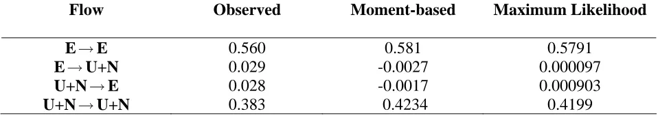
Table 9: Observed and adjusted, using the moment-based and the maximum likelihood estimators, labour force gross flows from the US CPS under intense misclassification

Flow Observed Moment-based Maximum Likelihood

E→E 0.560 0.581 0.5791

E→U+N 0.029 -0.0027 0.000097

U+N→E 0.028 -0.0017 0.000903

[image:26.595.67.546.674.759.2]

The existence of measurement error when estimating labour force gross flows leads to an overestimation of the labour market mobility. The effect of adjusting labour force gross flows for measurement error is to increase the diagonal elements and decrease the off-diagonal elements of the unadjusted gross flows matrix. This is consistent with the results of previous research (Poterba and Summers 1986; Singh and Rao 1995). The higher efficiency of the maximum likelihood estimator, compared to the moment-based estimator, is further illustrated in Table 8 by examining the estimated standard deviations. However, here we should also account for the fact that the variance estimator of the maximum likelihood estimator, using the Missing Information Principle, overestimates the true variance of this estimator (see Simulation V in Section 5). Last but not least, assuming that the adjusted estimates are unbiased, both the moment-based and the maximum likelihood estimators outperform the unadjusted estimator in Mean Squared Error terms.

In the second application we contrasted the moment-based estimator with the maximum-likelihood estimator in the presence of “intense” misclassification. Even a relatively small change in an entry of the original misclassification matrix is capable of causing the moment-based estimator to produce estimates that lie outside the boundaries of the parameter space (Table 9). This is partially due to the inversion of the misclassification matrix involved in deriving the moment-based estimates (Section 3.1). A further reason, however, is the use of the ICE assumption. The effect of the ICE assumption is to overestimate the panel misclassification error compared to a case where serial correlation in the misclassification error exists. Unlike the moment-based estimator, the maximum likelihood estimator constrains the adjusted estimates to lie within the boundaries of the parameter space.

7. Summary

the context of a missing data problem. Monte-Carlo simulation results verify that the likelihood-based approach offers significant gains in efficiency over the moment-likelihood-based method. This is true under alternative double sampling designs. Variance estimation is considered and the proposed variance estimators appear to have good coverage properties. Using a real data application we illustrate that under certain conditions the moment-based estimator can produce estimates that lie outside the boundaries of the parameter space. Unlike the moment-based estimator, the maximum likelihood estimator constraints the adjusted estimates to lie within the boundaries of the parameter space. Based on the increased efficiency and the desirable numerical properties of the maximum likelihood estimator, we propose that this estimator should be preferred over the moment-based estimator.

Currently, we investigate the application of this methodology in other areas of statistical research such as in demographic applications for tackling the problem of heaping and in statistical disclosure control for protecting sensitive data via the introduction of misclassification error.

ACKNOWLEDGEMENT

The author would like to thank Ray Chambers for his guidance and helpful comments. The work in this paper was supported by the Economic and Social Research Council through award S42200034035.

APPENDIX A: PROOFS OF RESULTS IN SECTION 3 Proof of Result 3.1

Recalling the notation from Section 3, the expectations of the missing data can be expressed as follows:

E n

( )

_ij( )∗ =nE Y

(

_{ξt t→+1} =i Y, _ξ∗_{t t→+1} = j

)

. (A.1)

)

=

Expression (A.1) is re-defined below

(

) (

2

1 1 1

1 | . ∗ →+ →+ →+ = =

∑

= = i r

j t t t t t t

i

n n E Y_ξ j Y_ξ i E Y_ξ =i

)

)

)

Given the observed data, the conditional expectations of the missing data are expressed as follows

(

( )

)

(

) (

(

) (

2

1 1 1

1 1 1

1 | | . | ∗ →+ →+ →+ ∗ ∗ →+ →+ →+ = ⎡ ⎤ ⎢ ⎥ ⎢ = = = ⎥ ⎢ ⎥ = _{⎢ ⎥} ⎢ _{= = =} ⎥ ⎢ ⎥ ⎣

∑

⎦ i

t t t t t t

m

ij j _r

t t t t t t

i

E Y j Y i E Y i

E n D n

E Y j Y i E Y i

ξ ξ ξ

ξ ξ ξ

(A.2)

The expectations of the random variables involved in the expression above are determined using results for binomial random variables. More specifically,

E Y

(

_ξ∗_{t t→+1} = j Y| _{ξt t→+1} =i

)

=q_ij, E Y

(

_{ξt t→+1} =i

)

=P_i . (A.3) Substituting (A.3) in (A.2) we obtain the required result

(

( ) ( )

)

( ) ( ) ( ) ( ) 2 1 | , ∧ ∧ ∧ ∗ ∧ ∧ = ⎛ _⎞⎟ ⎜ _⎟ ⎜ _⎟ ⎜ _⎟ ⎜ _⎟ ⎜ = _⎜ ⎟_⎟ ⎜ _⎟⎟ ⎜ _⎟ ⎜ _⎟ ⎜ ⎟ ⎝

∑

⎠ i h h i ij h m

ij j _{r h}

h i ij i

q P

E n D n

q P Θ .

)

. ∗ ₌

)

=

)

= t

)

)

Proof of Result 3.2

Using the same notation as in Result 3.1, the expectations of the missing data in the validation sample are expressed as

E n

(

ijv( )

)

n E Yv

(

t t 1 i Y, t t 1 j (A.4)

∗

→+ →+

= _ξ = _ξ

Expression (A.4) is re-defined below

E n

(

ijv( )

)

n E Yv

(

t t 1 j Y| t t 1 i E Y

) (

t t 1 i .

∗ ∗

→+ →+ →+

= _ξ = _ξ = _ξ

For the validation sample we have information about the cross-sectional incidence of error _kv = v

∑ ∑

(

∗_{t t→+1} = | _{t t→+1} =

) (

_t→+1 .

i j

n n E Yξ j Yξ i E Yξ i

Given the observed data, the conditional expectations of the missing data are expressed as follows

(

( )

)

(

) (

(

) (

2 2

1 1 1

1 1 1

1 1 | | . | ∗ →+ →+ →+ ∗ ∗ →+ →+ →+ = = ⎡ ⎤ ⎢ ⎥ ⎢ = = = ⎥ ⎢ ⎥ = _{⎢ ⎥} ⎢ _{= = =} ⎥ ⎢ ⎥ ⎢ ⎥ ⎣

∑ ∑

⎦

t t t t t t

v v v

ij k _{r r}

t t t t t t

j i

E Y j Y i E Y i

E n D n

E Y j Y i E Y i

ξ ξ ξ

ξ ξ ξ