Adaptive near minimum error rate training for neural networks with application to multiuser detection in CDMA communication systems

Signal Processing 85 (2005) 1435–1448

Adaptive near minimum error rate training for neural

networks with application to multiuser detection in

CDMA communication systems

S. Chen

, A.K. Samingan, L. Hanzo

School of Electronics and Computer Science, University of Southampton, Highfield, Southampton SO17 1BJ, UK

Received 2 October 2003; received in revised form 24 February 2005

Abstract

Adaptive training of neural networks is typically done using some stochastic gradient algorithm that aims to minimize the mean square error (MSE). For many classification applications, such as channel equalization and code-division multiple-access (CDMA) multiuser detection, the goal is to minimize the error probability. For these applications, adopting the MSE criterion may lead to a poor performance. A nonlinear adaptive near minimum error rate algorithm called the nonlinear least bit error rate (NLBER) is developed for training neural networks for these kinds of applications. The proposed method is applied to downlink multiuser detection in CDMA communication systems. Simulation results show that the NLBER algorithm has a good convergence speed and a small-size radial basis function networktrained by this adaptive algorithm can closely match the performance of the optimal Bayesian multiuser detector. The results also confirm that training the neural networkmultiuser detector using the least mean square algorithm, although generally converging well in the MSE, can produce a poor error rate performance. r2005 Elsevier B.V. All rights reserved.

Keywords:Neural networks; Adaptive algorithms; Mean square error; Error probability; CDMA; Multiuser detectors; Bayesian detector

1. Introduction

We consider a class of neural networkclassifiers where pattern vectors are drawn from a finite set and corrupted by an additive noise. Examples include neural networkequalizers and multiuser

detectors in communication systems [1–15]. Typi-cally, sample-by-sample adaptation is needed for practical applications to meet real-time computa-tional constraints, and the training of neural networkclassifiers is usually done using some stochastic gradient algorithm based on the mean square error (MSE) criterion. It is often reported that a nonlinear classifier (e.g. a neural network equalizer or multiuser detector) can provide a www.elsevier.com/locate/sigpro

0165-1684/$ - see front matterr2005 Elsevier B.V. All rights reserved. doi:10.1016/j.sigpro.2005.02.005

considerable performance improvement over a linear one. However, a close examination of the literature shows that the reported results are often inconsistent, namely many of these reported works do not compare the classification performance of their neural networks with the potentially achiev-able optimal performance for the given classifier structure. As pointed out by Pados and Papantoni-Kazakos [16], a strange situation exists that, on one hand, the performance of a classifier is evaluated using probability of error while, one the other hand, a different MSE criterion is used at the learning stage.

For linear classifiers, such as linear equalizers and code-division multiple-access (CDMA) mul-tiuser detectors, there is a partial relationship between the MSE and the error probability. A small MSE is usually associated with a small error rate. However, even in the linear case, the minimum MSE (MMSE) solution in general is not the minimum error rate (MER) solution. For the linear equalizer or multiuser detector with binary signalling, it is now well-known that the bit error rate (BER) difference between the MMSE solution and the minimum BER (MBER) one can be large in certain situations [17–29]. Recent research has aimed to develop adaptive linear equalizer and multiuser detector based on the

MBER criterion [20,22,25–29]. For nonlinear

classifiers, the relationship between the MSE and the error rate is more dubious, and the MMSE solution does not necessarily correspond to a small error rate.1In effect, standard adaptive algorithms for training nonlinear classifiers, such as the least mean square (LMS) algorithm, is based on a criterion that may not be relevant to the true performance indicator. Notice that this scenario exists only for the adaptive learning case.

For off-line or block-data based learning, the need for adopting a relevant criterion to train classifiers has always been recognized. Given the underlying pattern space, that is, the information available to a classifier, the maximum a posteriori

probability or Bayesian classifier provides the true optimal performance. The definition of the MER used in this paper is referred to the achievable error rate for a classifier with an additional constraint of a given structure (e.g. a radial basis function (RBF) classifier with a given number of hidden nodes). The basic question is then whether it is possible to achieve this MER and how close it is to the true performance of the Bayesian classifier. It is not surprising that the Bayesian learning approach is the most general block-data based method for training a nonlinear classifier with given structure. Typical Bayesian learning algorithms include the so-called type-II maximum likelihood or evidence procedure [30,31], and the Markov chain Monte Carlo sampling method[32]. If the classifier has a special structure of a kernel representation, the support vector machine [33]

and the relevance vector machine[34]have become popular. All these training algorithms suffer from high computational costs and cannot be imple-mented in a true adaptive sample-by-sample training manner.

The main contribution of this paper is to develop an adaptive near MER training algorithm for a class of neural networkclassifiers that includes nonlinear equalizers and multiuser detec-tors. It should be pointed out that adaptive near MER training can in theory be achieved by only adjusting the classifier parameters when a classifi-cation error occurs. However, for appliclassifi-cations considered in this paper, error rate is typically very small. This strategy is impractical, since it would require an extremely long training period. The approach adopted in this paper is based on a Parzen window or kernel density estimation

[35–37]to approximate the error rate from training data and to derive a stochastic gradient adaptive algorithm. The resulting algorithm will be called the nonlinear least error rate (NLER) algorithm. In channel equalization and multiuser detection applications with binary modulation schemes, this NLER algorithm will be referred to as the nonlinear least bit error rate (NLBER). The algorithm is used to train downlinkRBF multiuser

detectors in CDMA communication systems

[38,39]. Convergence rate of the NLBER algo-rithm is investigated in simulation, and BERs of

the RBF multiuser detector trained by the LMS and NLBER algorithms are compared with those of the optimal Bayesian multiuser detector. The results obtained show that the NLBER algorithm achieves consistent performance and has a reason-able convergence speed. A small-size RBF network trained by the NLBER algorithm can closely approximate the optimal Bayesian detector. The simulation study also demonstrates that the RBF networktrained by the LMS algorithm, although converging consistently in the MSE, can produce poor BER performance.

2. Adaptive near minimum error rate training

Consider a class of nonlinear classifiers that can be represented by

^

cðkÞ ¼sgnðyðkÞÞwithyðkÞ ¼fðrðkÞ;wÞ, (1) wherekindicates the sample number,rðkÞis an M-dimensional pattern vector with its associated class labelcðkÞ 2 f1g;fð;Þdenotes the classifier map,

the vector w consists of all the (adjustable)

parameters of the classifier, and c^ðkÞ is the estimated class label for rðkÞ: The pattern vector

rðkÞis assumed to take the form

rðkÞ ¼¯rðkÞ þnðkÞ, (2) where the ‘‘clean’’ or noise-free part r¯ðkÞ takes values from a finite set with equal probability

¯

rðkÞ 2 f¯rj; 1pjpNbg (3)

and the noise vector nðkÞ is white Gaussian with covariance matrix E½nðkÞnTðkÞ ¼s2

nI; I being an identity matrix of appropriate dimension. Each¯rj has an associated class labelcðjÞ _{2 f1g:}

A usual way of training such a nonlinear classifier is to adjust the classifier’s parameters w

so that the MSE

E½ðcðkÞ yðkÞÞ2 (4)

is minimized. Typically, a stochastic gradient algorithm called the LMS can be used in adaptive implementation, and the algorithm has a simple form

yðkÞ ¼fðrðkÞ;wðk1ÞÞ,

wðkÞ ¼wðk1Þ þmðcðkÞ yðkÞÞqfðrðkÞ;wðk1ÞÞ qw ,

ð5Þ

where m is an adaptive gain. However, the true

performance criterion is the error rate and it is desirable to develop an adaptive training algo-rithm based on the MER criterion. We will first consider the theoretical error rate of the classifier (1) and a block-data based training. This will provide insight into the development of our adaptive near MER training algorithm.

2.1. An approximate error rate expression

As an error only occurs when the sign ofyðkÞis different from sgnðcðkÞÞ; the error probability of the classifier (1) is

PEðwÞ ¼ProbfsgnðcðkÞÞyðkÞo0g. (6)

Define the signed variable

y_sðkÞ ¼sgnðcðkÞÞyðkÞ (7)

and let the probability density function (p.d.f.) of y_sðkÞbep_yðy_sÞ:Then

PEðwÞ ¼ Z 0

1

p_yðy_sÞdy_s. (8)

By linearizing the classifier around ¯rðkÞ;it can be approximated as2

yðkÞ ¼fð¯rðkÞ þnðkÞ;wÞ fð¯rðkÞ;wÞ

þ qfðr¯ðkÞ;wÞ qr

T

nðkÞ

¼fð¯rðkÞ;wÞ þeðkÞ, ð9Þ

where eðkÞ is Gaussian with zero mean and

variance

r2_{ðwÞ ¼E s}2

n

qfðr¯ðkÞ;wÞ qr

T

qfð¯rðkÞ;wÞ qr

" #

¼ s

2

n Nb

XNb

j¼1

qfðr¯j;wÞ qr

T

qfð¯rj;wÞ

qr . ð10Þ

Essentially, the classifier is approximated as an additive Gaussian noise model

yðkÞ ¯yðkÞ þeðkÞ (11)

when deriving its error rate expression, with ¯yðkÞ taking values from the finite set

¯yðkÞ 2 f¯yj¼fð¯rj;wÞ; 1pjpNbg. (12)

The p.d.f. ofy_sðkÞcan thus be approximated by

p_yðy_sÞ 1 Nb

ffiffiffiffiffiffi 2p

p

rðwÞ XNb

j¼1

exp ðyssgnðc ðjÞ_Þ¯y

jÞ2 2r2_ðwÞ

!

(13)

and the error probability of the classifier is approximately

PEðwÞ 1 Nb

ffiffiffiffiffiffi 2p

p X

Nb

j¼1

Z 1

gjðwÞ

exp x

2

j 2

! dxj

¼ 1

Nb XNb

j¼1

Qðg_jðwÞÞ, ð14Þ

where

QðxÞ ¼ 1_{ffiffiffiffiffiffi} 2p

p Z 1

x

exp y

2

2

dy (15)

and

g_jðwÞ ¼sgnðc ðjÞ_Þ¯y

j

rðwÞ ¼

sgnðcðjÞÞfðr¯j;wÞ

rðwÞ . (16)

The linearization (9) is valid only for smallnðkÞ (in some statistical sense), but the assumption of small nðkÞ usually holds in practice. In general, however, the error rate expression (14) is a good approximation of the true error probability, and minimizing this approximate error rate expression will lead to a near MER solution.

2.2. Approximate minimum error rate solution

If the set described by (3) is known (for example, in equalization application if the channel impulse response (CIR) is known), an approximate MER solution can be obtained by minimizing the

approximate error rate expression (14) numeri-cally. The gradient ofPEðwÞis approximately

rPEðwÞ 1 Nb

ffiffiffiffiffiffi 2p

p X

Nb

j¼1

exp ¯y

2

j 2r2

! qgjðwÞ

qw

1 Nb

ffiffiffiffiffiffi 2p

p

r

XNb

j¼1

exp ¯y

2

j 2r2

!

sgnðcðjÞÞqfð¯rj;wÞ

qw . ð17Þ

In the above second approximation, we have dropped the term containingqr=qw:The following iterative steepest-descent gradient algorithm can be used to arrive at an approximate MER solution. Given an initial wð0Þ; at lth iteration, the algorithm computes

¯y_jðlÞ ¼fðr¯j;wðl1ÞÞ; 1pjpNb,

rPEðwðlÞÞ ¼ 1 Nb

ffiffiffiffiffiffi 2p

p

r

XNb

j¼1

exp ¯y

2

jðlÞ 2r2

!

sgnðcðjÞÞqfð¯rj;wðl1ÞÞ qw ,

wðlÞ ¼wðl1Þ mrPEðwðlÞÞ, (18)

where m is a step size. Since PEðwÞ is a highly

complex nonlinear function of w; a

steepest-descent gradient algorithm may converge slowly. A simplified conjugate gradient algorithm [28,40]

with a periodical resetting of the search direction to the negative gradient can alternatively been used to speed up convergence.

Assuming qr=qw¼0 is to assume that the

2.3. Block-data based gradient adaptation

In practice, the set of¯rjis unknown. The key to developing an effective adaptive algorithm is the p.d.f.p_yðy_sÞ of the decision variable y_sðkÞ: Parzen window or kernel density estimation [35–37] is a well-known method for estimating a probability distribution. Parzen window method estimates a p.d.f. using a window or blockofysðkÞby placing a symmetric unimodal kernel function (such as the Gaussian function) on each y_sðkÞ: This kernel density estimation is capable of producing reliable p.d.f. estimates with short data records and in particular is extremely natural when dealing with

Gaussian mixtures. Given a blockof K training

samplesfrðkÞ;cðkÞgK_k¼1;a kernel density estimate of the true p.d.f.p_yðy_sÞis readily given by

^

pyðysÞ ¼ 1 Kpffiffiffiffiffiffi2pr¯

XK

k¼1

exp ðyssgnðcðkÞÞyðkÞÞ

2

2¯r2

,

(19)

where the kernel width r¯ is an appropriately

chosen positive constant. From the estimated p.d.f. (19), an estimated error probability

^

PEðwÞ ¼ Z 0

1

^

p_yðy_sÞdy_s (20)

is obtained, and its gradient rP^EðwÞ can be calculated exactly according to

rP^EðwÞ ¼ 1 Kpffiffiffiffiffiffi2pr¯

XK

k¼1

exp y

2_ðkÞ

2r¯2

sgnðcðkÞÞqfðrðkÞ;wÞ

qw . ð21Þ

Thus a block-data based adaptive steepest-descent gradient algorithm can be derived. Atlth iteration, the algorithm computes

yðkÞ ¼fðrðkÞ;wðl1ÞÞ; 1pkpK,

rP^EðwðlÞÞ ¼ 1 Kpffiffiffiffiffiffi2pr¯

XK

k¼1

exp y

2_ðkÞ

2r¯2

sgnðcðkÞÞqfðrðkÞ;wðl1ÞÞ qw ,

wðlÞ ¼wðl1Þ mrP^EðwðlÞÞ, (22)

where the adaptive gain mand the kernel width r¯ are the two algorithm parameters that require tuning. Specifically, m and r¯ control the rate of convergence, and r¯ also helps to determine the accuracy of the p.d.f. and hence error rate estimate. Alternatively, conjugate gradient based adaptation can be adopted.

Several critical points need to be emphasized.

Provided that the kernel width r¯ is chosen

appropriately, the Parzen window estimate (19) is an accurate estimate of the true density p_yðy_sÞ regardless whether the approximation (13) is valid or not. Accuracy analysis of Parzen window density estimate is well documented in the literature. The p.d.f. estimate (19) is known to possess a mean integrated square error conver-gence rate at order ofK1 _{[35]and it can achieve} an accurate estimate with a remarkably short data record. It is also worth re-iterating that the gradient (21) is exact and involves no approximation.

2.4. Stochastic gradient adaptation

Our aim is to develop a stochastic gradient adaptive algorithm with sample-by-sample updat-ing, in a similar manner to the LMS (5). The LMS algorithm is derived from its related ensemble gradient algorithm by replacing the ensemble average of the gradient with a single data point estimate of the gradient. Adopting a similar strategy, at samplek, a single-data-point estimate of the p.d.f. is

^

p_yðy_s;kÞ ¼ _{ffiffiffiffiffiffi}1 2p

p ¯

rexp

ðy_ssgnðcðkÞÞyðkÞÞ2 2r¯2

.

(23)

Using the instantaneous or stochastic gradient

rP^Eðk;wÞ ¼ 1 ffiffiffiffiffiffi 2p

p ¯

rexp

y2_ðkÞ 2r¯2

sgnðcðkÞÞqfðrðkÞ;wÞ

qw ð24Þ

a stochastic gradient algorithm is readily given by

wðkÞ ¼wðk1Þ þ _{ffiffiffiffiffiffi}m 2p

p ¯

rexp

y2_ðkÞ 2r¯2

sgnðcðkÞÞqfðrðkÞ;wðk1ÞÞ

qw , ð25Þ

where the adaptive gainm and the kernel widthr¯ are the two algorithmic parameters that have to be set appropriately. Specifically, they are chosen to ensure adequate performance in terms of conver-gence rate and steady-state error rate misadjust-ment.

Following a similar reasoning to the LMS for the MMSE criterion, the algorithm (25) will be called the NLER for the near MER criterion. Specially, in equalization and multiuser detection applications involving binary signalling, this sto-chastic gradient algorithm will be called the NLBER for the near MBER criterion.

3. Adaptive training of neural network multiuser detectors

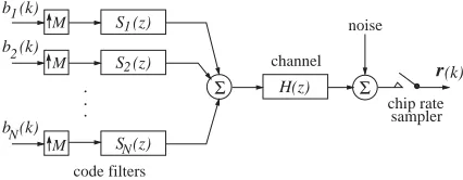
The performance of the NLBER algorithm (25) is investigated in an application to multiuser detection in the CDMA downlink(base station to mobile), in which a detector estimates the transmitted information bits of a desired user in the presence of interfering users.

3.1. Synchronous CDMA downlink system model

Using notations from the multi-rate filtering literature[41], the discrete-time baseband model of the synchronous CDMA downlinksystem

sup-porting N users with M chips per symbol is

depicted inFig. 1, wherebiðkÞ 2 f1gdenotes the

kth symbol of user i, the unit-length signature sequence for user iis

~

si¼ ½s~i;1 s~i;MT (26) and the transfer function of the CIR at the chip rate is

HðzÞ ¼X nh1

i¼0

hizi. (27)

The baseband model for received signal sampled at chip rate is given by [42,43]

rðkÞ ¼P

bðkÞ

bðk1Þ

.. .

bðkLþ1Þ 2 6 6 6 6 6 4 3 7 7 7 7 7 5

þnðkÞ ¼¯rðkÞ þnðkÞ,

(28)

where the user symbol vector bðkÞ ¼

½b1ðkÞ bNðkÞT; the white Gaussian noise vec-tor nðkÞ ¼ ½n1ðkÞ nMðkÞT with E½nðkÞnTðkÞ ¼

s2

nI;r¯ðkÞdenotes the noise-free received signal, and

theMLN system matrixPhas the form

P¼H ~

SA 0 0

0 SA~ .. . ... .. . . . . . . . 0 0 0 SA~

2 6 6 6 6 6 4 3 7 7 7 7 7 5 (29)

with theMLM CIR matrixH given by

H¼

h0 h1 hnh1

h0 h1 hnh1

. . .

. . .

.. . h0 h1 hnh1

2 6 6 6 6 6 4 3 7 7 7 7 7 5 (30)

the normalized user code matrix given by S~ ¼

½s~1 ~sN;and the diagonal user signal amplitude matrix given by A¼diagfA1 ANg:The chan-nel intersymbol interference spanLdepends on the

CIR length nh and the chip sequence length M:

L¼1 for nh ¼1;L¼2 for 1onhpM;L¼3 for Monhp2M;and so on.

The detector at the receiver for user iestimates the transmitted bit biðkÞ based on the received H(z)

M

M

S (z)

S (z)

. . .

S (z)

N 2 1

Σ

b (k)_N b (k) b (k)₁

2 r(k) chip rate channel code filters M sampler noise Σ

signalrðkÞ;and has a general form of

^

biðkÞ ¼sgnðyðkÞÞwithyðkÞ ¼fðrðkÞ;wÞ, (31) wherewis the detector parameter vector for useri. This is obviously an example of the classifier discussed in the previous section withbiðkÞserving as the class label for rðkÞ: Let the Nb¼2LN

possible combinations or sequences of

½bTðkÞbTðk1Þ bTðkLþ1ÞTbe

bðjÞ¼

bðjÞðkÞ

bðjÞðk1Þ

.. .

bðjÞðkLþ1Þ 2

6 6 6 6 6 4

3 7 7 7 7 7 5

; 1pjpNb (32)

andbðjÞ_i theith element of bðjÞðkÞ:Define the set of Nb noise-free received signal states

R¼ f¯rj ¼PbðjÞ; 1pjpNbg (33)

and the set ofNb scalars

f¯yj¼fð¯rj;wÞ; 1pjpNbg. (34) Notice that¯rðkÞcan only take the values from the setR;the class label for¯rjisbðjÞi 2 f1gfor useri, andRcan be divided into two subsets

R¼ f¯rj 2R: bðjÞi ¼ 1g. (35)

3.2. Linear and optimal detectors

A linear detector for user i has the decision variable given by

y_LðkÞ ¼f_LðrðkÞ;wÞ ¼wTrðkÞ. (36) The most popular solution for this linear detector

is the MMSE one given[42,44–47]

wMMSE¼ ðs2nIþPPTÞ 1_p

i, (37)

wherep_iis theith column ofP:More recently, the linear MBER solution for the linear detector (36) has been derived [28]. However, a linear detector

only performs adequately if Rþ and R are

linearly separable. IfRþ and R are not linearly separable, a linear detector will have a high BER floor even without noise and a nonlinear detector will be required[48]. Even in the case thatRþ and Rare linearly separable, a nonlinear detector can

often outperform a linear one considerably at a cost of increased complexity.

Applying the maximum a posteriori probability principle, it can be shown that the optimal one-shot detector is the following Bayesian one [48]:

y_BðkÞ ¼f_BðrðkÞ;wÞ ¼ X

rj2R

xjbðjÞi

ð2ps2

nÞ M=2

exp krðkÞ ¯rjk

2

2s2

n

, ð38Þ

where xj are a priori probabilities of ¯rj and, since all the r¯j are equiprobable, xj ¼1=Nb: The Bayesian decision variable can also be written as

y_BðkÞ ¼f_BðrðkÞ;wÞ ¼X Nb

j¼1

b_jexp krðkÞ ¯rjk

2

2s2

n

(39)

with

bj¼

bðjÞ_i Nbð2ps2nÞ

M=2. (40)

Notice that, for binary data symbols f1g; multi-plying allb_j by any positive constant still gives the same optimal Bayesian solution, and the perfor-mance of the Bayesian solution is insensitive to whether a precise noise variance or an estimate is used [49,50]. For example, substituting s2

n in (39) by, say, 0:5s2

n or 2s2n; the BER performance are indistinguishable from the exact Bayesian solution. Implementation of the optimal Bayesian detector (39) is computationally very expensive with the associated difficulty of adaptively estimating the set of noise-free signal states (33).

3.3. Adaptive radial basis function network detector

To test the NLBER algorithm for adaptive training of neural networkmultiuser detectors, we choose the RBF networkdetector of the form

y_RBFðkÞ ¼f_RBFðrðkÞ;wÞ

¼ X

nc

j¼1

ajexp

krðkÞ cjk2

~

sj

. ð41Þ

The parameter vector w contains all the RBF

ofw is thereforeNp¼nc ðMþ2Þ:It should be emphasized that other neural networks, such as the multilayer perceptron or the polynomial kernel function networkof the form

y_PolðkÞ ¼f_PolðrðkÞ;wÞ ¼X np

j¼1

ajðcTjrðkÞ þ1Þ

d ₍₄₂₎

can similarly be used as multiuser detectors. A reason for using the RBF network(41) in this study is that we would like to investigate whether the NLBER algorithm can achieve the optimal Bayesian performance when the form and size of the detector is similar to that of the Bayesian detector.

To implement an adaptive algorithm, such as the LMS or NLBER, the derivatives of the detector with respect to the detector parameters are required. For the RBF network(41), these derivatives can readily be calculated:

qf_RBF qaj

¼exp krðkÞ cjk

2

~

sj

qf_RBF qs~j

¼ajexp

krðkÞ cjk2

~

sj

_{krðkÞ c}

jk2

~

s2_j

qf_RBF qcj

¼2ajexp

krðkÞ cjk2

~

sj

_rð

kÞ cj

~

sj 9 > > > > > > > > > > = > > > > > > > > > > ;

1pjpnc. ð43Þ

Both the LMS and NLBER algorithms are used to train the RBF networkdetector with the adaptive gainmgiven in the formmk¼m0k1=4;wherem0 is

an appropriately chosen constant. For the

NLBER algorithm, the value of r¯2 also needs to be determined. In the simulation study,m0 andr¯2 are chosen empirically. Specifically, m₀ is chosen for the LMS algorithm to ensure fast convergence speed and a small steady-state MSE, whilem₀ and ¯

r2_{are chosen for the NLBER algorithm to achieve}

fast convergence rate and a small

steady-state BER.

3.4. Simulation study

In all simulations, the firstnc=2 data points that belong to the class þ1 and the first nc=2 data

points that belong to the class 1 are used as

initial centers. The initial weights are set to Z

accordingly, where Z is a small positive number. To take into account the influence of initial centers, the algorithm are run many times with different random initializations for different runs.

All the RBF widths are initially set to 8s2

n; assuming an estimated noise variance of 4s2_n: Two kinds of BER are mentioned in the results, the true BER that is computed using Monte Carlo simulation with a sufficiently long test sequence and the estimated BER calculated using the approximate BER expression (14) with g_jðwÞ ¼ sgnðbðjÞ_i Þ¯yj=r~:The value ofr~2is fixed such that, for k¼0 andkequal to the final training sample, the estimated BERs agree with the true BERs. This r~

should not be confused with the NLBER

algo-rithm parameter r¯ used in adaptation. The

estimated BER is used to illustrate the learning rate of an adaptive algorithm, providing an ‘‘estimate’’ for PEðwðkÞÞ; the true BER of the detector with the weight vector wðkÞ; at each

training sample k. An alternative would be to

provide the true learning rate of the algorithm. This would require to calculate the true BER using Monte Carlo simulation at each training samplek, which is computationally too demanding, if not impossible.

Example 1. This was a very simple two-user system with 2 chips per symbol. The code

sequences of the two users were ð1;1Þ and

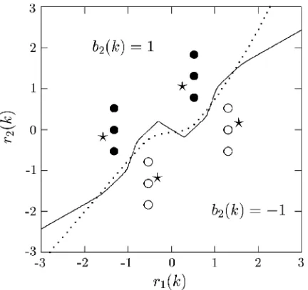
ð1;þ1Þ;respectively, and the transfer function of the CIR at chip rate wasHðzÞ ¼1:0þ0:4z1_:The two users had equal signal power, that is, the user 1 signal to noise ratio SNR1was equal to SNR2of user 2. The setRhad 16 points, but only 12 were distinct. This example was chosen to demonstrate that multiuser detection can be considered as a classification problem, as a two-dimensional space can graphically be illustrated. The system was so

set up to ensure that Rþ and R were linearly

separable and hence a linear detector could work adequately. Fig. 2displaysRþ andR for user 2 together with the two decision boundaries of the linear MBER and optimal Bayesian detectors for a SNR2¼17 dB (corresponding to a user 2 signal to

interference plus noise ratio of SINR2 ¼

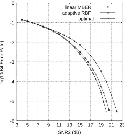
optimal Bayesian detectors are depictedin Fig. 3

for user 2 given the range of SNR2from 3 to 23 dB (SINR2 from1:76 to0:02 dB).

Given SNR2¼17 dB;RBF detectors with 4 and 12 centers were trained by the LMS and NLBER algorithms, respectively. The NLBER had r¯2 _¼ 4s2

n for both detectors, and m0¼0:2 for the 4-center RBF and m₀¼0:25 for the 12-center RBF; while the LMS hadm0¼0:1 for the 4-center RBF and m0¼0:3 for the 12-center RBF. These values were found empirically to be appropriate. At each sample k, the estimated BER was calculated for a detector withwðkÞ;and this resulted in the learning rates, plotted inFig. 4, for the respective detectors, where the results were averaged over 100 runs. For the LMS training, the MSE for a detector with

wðkÞwas also calculated using a blockof 100 test samples, and this produced the learning rates in terms of the MSE given inFig. 5, whereagain the results were averaged over 100 runs. The decision boundary of a typical 4-center RBF detector trained by the NLBER algorithm is compared with the optimal Bayesian boundary inFig. 6.

The learning rates for the estimated BER given in Fig. 4 need some explanations. It was found that the estimated BERs of the 4-center RBF detector with the LMS training varied greatly for different runs. For some runs the estimated BERs were close to that obtained by the average NLBER training (0.001), but for other runs the estimated

Fig. 2. The set of noise-free signal points and the two decision boundaries (dotted: linear MBER, solid: optimal) for user 2 of Example 1. SNR1¼SNR2¼17 dB:

-6 -5 -4 -3 -2 -1 0

3 5 7 9 11 13 15 17 19 21 23

log10(Bit Error Rate)

SNR2 (dB) linear MBER adaptive RBF optimal

Fig. 3. Performance comparison of three detectors for user 2 of Example 1. SNR1¼SNR2:The adaptive RBF detector has 4

centers and is trained by the NLBER algorithm.

0.0001 0.001 0.01 0.1 1 10

0 200 400 600 800 1000

Estimated Bit Error Rate

Sample k 4-LMS 12-LMS 4-LBER 12-LBER

Fig. 4. Learning curves in terms of the estimated BER for user 2 of Example 1. SNR1¼SNR2¼17 dB: The results are

averaged over 100 runs. 4-LMS: the 4-center RBF trained by the LMS with m₀¼0:1; 12-LMS: the 12-center RBF trained by the LMS withm0¼0:3;4-LBER: the 4-center RBF

trained by the NLBER with m0¼0:2 andr¯2¼4s2n; and

12-LBER: the 12-center RBF trained by the NLBER withm0¼

0:25 andr¯2_¼4s2

BERs converged to 0.5. Examining the resulting RBF detectors for the latter case, it was seen that the 4 centers all converged to near the original with a symmetric configuration. This is not surprising, since this configuration can correspond to a small

MSE and is consistent with the LMS criterion. In fact, there was on average about 4 dB reduction in the MSE for the 4-center RBF detector trained by the LMS algorithm. Similar situations occurred for the 12-center RBF detector with the LMS training, and the averaged BER performance of the 12-center RBF trained by the LMS is poorer than that obtained for the 4-center detector trained by the NLBER. Note that this was more funda-mental than ‘‘local minima problem’’. In fact, examining the MSE learning rate for the 12-center RBF trained by the LMS, it was seen that different runs produced consistent performance and on average it had 11 dB reduction in the MSE. However, there was no direct linkbetween the MSE value and the BER. In comparison, the NLBER training was found to produce consistent BER results in different runs, and the 12-center RBF detector with the NLBER training converged consistently to the optimal Bayesian performance, in terms of BER.

The influence of the algorithm parameterr¯2 on the performance of the NLBER algorithm was also investigated. Fig.7 shows the (true) BERs of the 4-center RBF detector after the NLBER training with a range of r¯2_{;where it can be seen} that the algorithm performance is not overly sensitive to r¯2 _{over a large range of values. The} (true) BERs of the 4-center RBF detector after the NLBER training are depicted inFig. 3. The (true) 0.01

0.1 1

0 200 400 600 800 1000

Mean Square Error

Sample k 4-LMS 12-LMS

Fig. 5. Learning curves in terms of the MSE for user 2 of Example 1. SNR1¼SNR2¼17 dB:The results are averaged

over 100 runs. 4-LMS: the 4-center RBF trained by the LMS withm0¼0:1;and 12-LMS: the 12-center RBF trained by the

LMS withm0¼0:3:

Fig. 6. Comparison of two decision boundaries (dotted: adaptive RBF detector, solid: optimal) for user 2 of Example 1. SNR1¼SNR2¼17 dB:The adaptive RBF detector has 4

centers and is trained by the NLBER algorithm. The stars indicate the final center positions.

Fig. 7. Influence of r¯2 _{to the performance of the NLBER}

algorithm. User 2 of Example 1 with SNR1¼SNR2¼17 dB:

BERs of the 12-center RBF detector after the NLBER training are not shown here, as they are indistinguishable from the optimal performance. The 4-center RBF detector trained by the LMS did not workas the (true) BERs produced were often 50%, even though the algorithm converged well in the MSE. The (true) BERs of the 12-center RBF detector trained by the LMS algorithm, not shown here, were not much better than those of the linear MBER detector.

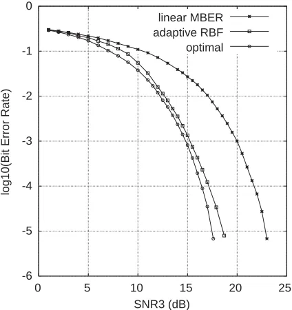
Example 2. Thiswas a 3-user system with 8 chips per symbol. The code sequences for the three users were ðþ1;þ1;þ1;þ1;1;1;1;1Þ; ðþ1;1; þ1;1;1;þ1;1;þ1Þ and ðþ1;1;1;þ1;1; þ1;þ1;1Þ;respectively, and the transfer function of the CIR at chip rate wasHðzÞ ¼0:8þ0:6z1_þ 0:5z2_{: The three users had equal signal power.} Again a linear separable situation was simulated. The detector for user 3 was considered, and the BERs of the linear MBER and optimal detectors are displayed inFig. 8for the range of SNR3from 0 to 25 dB (SINR3 from 4:77 to 3:02 dB). The noise-free state set R had 64 points. Given SNR3¼15 dB (SINR3¼ 3:08 dB), RBF

detec-tors with 16 and 64 centers were trained by the LMS and NLBER algorithms, respectively. The NLBER had r¯2_¼1000s2

nand m0 ¼0:6 for the 16-center RBF, and r¯2 _¼50s2

n and m0¼0:1 for the 64-center RBF; while the LMS had m0¼0:2 for the both RBF detectors. These values were found empirically to be appropriate. The learning rates in terms of the estimated BER are plotted in

Fig. 9 for the respective detectors, where the results were averaged over 100 runs. For the LMS training, the MSE convergence performance, averaged over 100 runs, are given inFig. 10.

The NLBER algorithm produced consistent results and, in particular, the 64-center detector was able to achieve the optimal performance in terms of BER. For the LMS training, the algorithm converged very well in the MSE and there was an almost 30 dB reduction in the MSE, as can be seen inFig. 10. However, the BERs of the two detectors trained by the LMS algorithm both approached to 0.5! In fact, averagely, the initial

16-center RBF detector had a BER¼0:2 and the

initial 64-center RBF detector had a BER¼0:008: Yet, after training using the LMS, both yielded almost 1 in 2 errors (not much better than a random guess). This clearly illustrates the fact that -6

-5 -4 -3 -2 -1 0

0 5 10 15 20 25

log10(Bit Error Rate)

SNR3 (dB) linear MBER adaptive RBF optimal

Fig. 8. Performance comparison of three detectors for user 3 of Example 2. SNRi;1pip3; are identical. The adaptive RBF

detector has 16 centers and is trained by the NLBER algorithm.

0.0001 0.001 0.01 0.1 1 10

0 400 800 1200 1600 2000

Estimated Bit Error Rate

Sample k 16-LMS 64-LMS

16-LBER 64-LBER

Fig. 9. Learning curves in terms of the estimated BER for user 3 of Example 2. SNRi¼15 dB; 1pip3: The results are

averaged over 100 runs. 16-LMS: the 16-center RBF trained by the LMS withm0¼0:2;64-LMS: the 64-center RBF trained

by the LMS with m0¼0:2; 16-LBER: the 16-center RBF

trained by the NLBER withm0¼0:6 andr¯2¼1000s2n;and

64-LBER: the 64-center RBF trained by the NLBER withm0¼0:1

andr¯2_¼50s2

a small MSE is not related to a small BER. As far as the LMS algorithm is concerned, it does a good job in what it supposes to do: getting the MSE down. The true BERs of the 16-center RBF detector after the NLBER training are compared with the optimal performance in Fig. 8, where it can be seen that its performance is very close to the optimal Bayesian detector of 64 states. The true BERs of the 64-center RBF detector trained by the NLBER, not depicted here, are indistinguishable from the optimal performance.

Example 3. The system had 4 equal power users with 8 chips per symbol. The code sequences for the four users were ðþ1;þ1;þ1;þ1;1;1; 1;1Þ;ðþ1;1;þ1;1;1;þ1;1;þ1Þ;ðþ1;þ1; 1;1;1;1;þ1;þ1Þ and ðþ1;1;1;þ1;1; þ1;þ1;1Þ;respectively, and the transfer function of the CIR at chip rate wasHðzÞ ¼0:4þ0:7z1_þ 0:4z2_{:The detector for user 2 was considered. For} user 2,RðþÞ andRðÞ are almost linearly insepar-able, and a linear detector has a relatively poor BER performance at low SNRs, as is shown in

Fig. 11. The BERs of the optimal Bayesian detector is also shown inFig. 11, where the range

of SNR2 from 10 to 30 dB corresponds to the

SINR2 from4:91 to 4:77 dB:Note that in this example the number of channel states Nb¼256; and the Bayesian detector is computationally very

expensive. The performance of the 64-center RBF detector trained by the NLBER algorithm is

depicted in Fig. 11. It can be seen that the

performance of this NLBER RBF detector is very close to the full optimal Bayesian performance. In the simulation it was again observed that the same 64-center RBF detector under the identical condi-tions but trained by the LMS algorithm, although converged well in the MSE, often resulted in BERs not much better than those of the linear MBER detector.

4. Conclusions

Adaptive training based on the MER criterion has been considered for a class of neural network classifiers that includes nonlinear equalizers and multiuser detectors. A main contribution of this research has been the derivation of an adaptive near MER algorithm called the NLER for this kind of applications. In the context of channel equalization and multiuser detection with binary modulation schemes, this adaptive algorithm has been referred to as the NLBER. Our approach has 1

10 100 1000

0 400 800 1200 1600 2000

Mean Square Error

Sample k 16-LMS 64-LMS

Fig. 10. Learning curves in terms of the MSE for user 3 of Example 2. SNRi¼15 dB; 1pip3: The results are averaged

over 100 runs. 16-LMS: the 16-center RBF trained by the LMS withm0¼0:2;and 64-LMS: the 64-center RBF trained by the

LMS withm0¼0:2:

-5 -4 -3 -2 -1 0

10 15 20 25 30

log10(BER)

SNR2 (dB) linear MBER adaptive RBF optimal

Fig. 11. Performance comparison of three detectors for user 2 of Example 3. SNRi;1pip4;are identical. The adaptive RBF

been motivated from a kernel density estimation of the error rate as a smooth function of the training data and an adoption of stochastic gradient of the estimated error probability. This adaptive algo-rithm has been applied to downlinkmultiuser detection in CDMA communication systems using a RBF network. Simulation results have demon-strated that the NLBER algorithm performs consistently and the algorithm has a good con-vergence speed. A small-size RBF detector trained by the NLBER algorithm can closely approximate the optimal Bayesian detector. When the size of the RBF detector is similar to the Bayesian

detector, the optimal performance can be

achieved. The results also demonstrate that the standard adaptive algorithm, the LMS, may not be very relevant for training neural networkclassi-fiers, as the underlying criterion of the LMS is the MSE not the error probability.

References

[1] S. Chen, G.J. Gibson, C.F.N. Cowan, P.M. Grant, Recursive prediction error algorithm for training multi-layer perceptrons, in: Proceedings of the IEEE Colloquium Adaptive Algorithms for Signal Estimation and Control, Edinburgh, Scotland, 1989, pp. 10/1–10/7.

[2] S. Chen, G.J. Gibson, C.F.N. Cowan, Adaptive channel equalization using a polynomial-perceptron structure, IEE Proc. Part I 137 (5) (1990) 257–264.

[3] S. Chen, G.J. Gibson, C.F.N. Cowan, P.M. Grant, Adaptive equalization of finite non-linear channels using multilayer perceptrons, Signal Processing 20 (2) (1990) 107–119.

[4] G.J. Gibson, S. Siu, S. Chen, C.F.N. Cowan, P.M. Grant, The application of nonlinear architectures to adaptive channel equalisation, in: Proceedings of ICC’90, Atlanta, USA, 1990, pp. 312.8.1–312.8.5.

[5] S. Siu, G.J. Gibson, C.F.N. Cowan, Decision feedback equalisation using neural networkstructures and perfor-mance comparison with the standard architecture, IEE Proc. Part I 137 (4) (1990) 221–225.

[6] S. Chen, G.J. Gibson, C.F.N. Cowan, P.M. Grant, Reconstruction of binary signals using an adaptive radial-basis-function equalizer, Signal Processing 22 (1) (1991) 77–93.

[7] G.J. Gibson, S. Siu, C.F.N. Cowan, The application of nonlinear structures to the reconstruction of binary signals, IEEE Trans. Signal Processing 39 (8) (1991) 1877–1884.

[8] B. Aazhang, B.P. Paris, G.C. Orsak, Neural networks for multiuser detection in code-division multiple-access

com-munications, IEEE Trans. Comm. 40 (7) (1992) 1212–1222.

[9] S. Chen, S. McLaughlin, B. Mulgrew, Complex-valued radial basis function network, Part II: application to digital communications channel equalisation, Signal Pro-cessing 36 (1994) 175–188.

[10] U. Mitra, H.V. Poor, Neural networktechniques for adaptive multiuser demodulation, IEEE J. Selected Areas Comm. 12 (9) (1994) 1460–1470.

[11] Z.J. Xiang, G.G. Bi, T. Le-Ngoc, Polynomial perceptrons and their applications to fading channel equalization and co-channel interference suppression, IEEE Trans. Signal Process. 42 (1994) 2470–2480.

[12] I. Cha, S.A. Kassam, Channel equalization using adaptive complex radial basis function networks, IEEE J. Selected Areas Comm. 13 (1) (1995) 122–131.

[13] C.H. Chang, S. Siu, C.H. Wei, A polynomial-perceptron based decision feedbackequalizer with a robust learning algorithm, Signal Processing 47 (1995) 145–158.

[14] D.G.M. Cruickshank, Radial basis function receivers for DS-CDMA, Electron. Lett. 32 (3) (1996) 188–190. [15] R. Tanner, D.G.M. Cruickshank, Volterra based receivers

for DS-CDMA, in: Proceedings of the 8th IEEE Interna-tional Symposium on Personal, Indoor and Mobile Radio Communications, vol. 3, September, 1997, pp. 1166–1170. [16] D.A. Pados, P. Papantoni-Kazakos, New nonleast-squares neural networklearning algorithms for hypothesis testing, IEEE Trans. Neural Networks 6 (3) (1995) 596–609. [17] E. Shamash, K. Yao, On the structure and performance of

a linear decision feedbackequalizer based on the minimum error probability criterion, in: Proceedings of ICC’74, 1974, pp. 25F1–25F5.

[18] S. Chen, E.S. Chng, B. Mulgrew, G.J. Gibson, Minimum-BER linear-combiner DFE, in: Proceedings of ICC’96, vol. 2, Dallas, Texas, 1996, pp. 1173–1177.

[19] N.B. Mandayam, B. Aazhang, Gradient estimation for sensitivity analysis and adaptive multiuser interference rejection in code-division multi-access systems, IEEE Trans. Comm. 45 (7) (1997) 848–858.

[20] C.C. Yeh, J.R. Barry, Approximate minimum bit-error rate equalization for binary signaling, in: Proceedings of ICC’97, vol. 2, Montreal, Canada, 1997, pp. 1095–1099. [21] S. Chen, B. Mulgrew, E.S. Chng, G.J. Gibson,

Space translation properties and the minimum-BER linear-combiner DFE, IEE Proc. Comm. 145 (5) (1998) 316–322.

[22] C.C. Yeh, R.R. Lopes, J.R. Barry, Approximate minimum bit-error rate multiuser detection, in: Proceedings of Globecom’98, Sydney, Australia, November 1998, pp. 3590–3595.

[23] S. Chen, B. Mulgrew, The minimum-SER linear-combiner decision feedbackequalizer, IEE Proc. Comm. 146 (6) (1999) 347–353.

[25] I.N. Psaromiligkos, S.N. Batalama, D.A. Pados, On adaptive minimum probability of error linear filter receivers for DS-CDMA channels, IEEE Trans. Comm. 47 (7) (1999) 1092–1102.

[26] B. Mulgrew, S. Chen, Stochastic gradient minimum-BER decision feedbackequalisers, in: Proceedings of IEEE Symposium on Adaptive Systems for Signal Processing, Communication and Control, Lake Louise, Alberta, Canada, October 1–4, 2000, pp. 93–98.

[27] C.C. Yeh, J.R. Barry, Adaptive minimum bit-error rate equalization for binary signaling, IEEE Trans. Comm. 48 (7) (2000) 1226–1235.

[28] S. Chen, A.K. Samingan, B. Mulgrew, L. Hanzo, Adaptive minimum-BER linear multiuser detection for DS-CDMA signals in multipath channels, IEEE Trans. Signal Process. 49 (6) (2001) 1240–1247.

[29] B. Mulgrew, S. Chen, Adaptive minimum-BER decision feedbackequalisers for binary signalling, Signal Processing 81 (7) (2001) 1478–1489.

[30] D.J.C. MacKay, Bayesian interpolation, Neural Compu-tation 4 (3) (1992) 415–447.

[31] D.J.C. MacKay, The evidence frameworkapplied to classification networks, Neural Computation 4 (1992) 720–736.

[32] X. Wang, R. Chen, Adaptive Bayesian multiuser detection for synchronous CDMA with Gaussian and impulsive noise, IEEE Trans. Signal Process. 47 (7) (2000) 2013–2028.

[33] V. Vapnik, The Nature of Statistical Learning Theory, Springer, New York, 1995.

[34] M.E. Tipping, Sparse Bayesian learning and the relevance vector machine, J. Mac. Learning Res. 1 (2001) 211–244. [35] E. Parzen, On estimation of a probability density function

and mode, Ann. Math. Statist. 33 (1962) 1066–1076. [36] B.W. Silverman, Density Estimation, Chapman & Hall,

London, 1996.

[37] A.W. Bowman, A. Azzalini, Applied Smoothing Techni-ques for Data Analysis, Oxford University Press, Oxford, UK, 1997.

[38] R. Prasad, CDMA for Wireless Personal Communica-tions, Artech House, Inc., 1996.

[39] S. Verdu´, Multiuser Detection, Cambridge University Press, Cambridge, UK, 1998.

[40] M.S. Bazaraa, H.D. Sherali, C.M. Shetty, Nonlinear Programming: Theory and Algorithms, Wiley, New York, 1993.

[41] P.P. Vaidyanathan, Multirate Systems and Filter Banks, Prentice-Hall, Englewood Cliffs, NJ, 1993.

[42] H.V. Poor, S. Verdu´, Probability of error in MMSE multiuser detection, IEEE Trans. Inform. Theory 43 (3) (1997) 858–871.

[43] B. Mulgrew, Nonlinear signal processing for adaptive equalisation and multi-user detection, in: Proceedings of EUSIPCO 98, Rhodes, Greece, September 1998, pp. 537–544.

[44] Z. Xie, R.T. Short, C.K. Rushforth, A family of suboptimum detectors for coherent multiuser communica-tions, IEEE J. Selected Areas Comm. 8 (4) (1990) 683–690. [45] U. Madhow, M.L. Honig, MMSE interference suppression for direct-sequence spread-spectrum CDMA, IEEE Trans. Comm. 42 (12) (1994) 3178–3188.

[46] S.L. Miller, An adaptive direct-sequence code-division multiple-access receiver for multiuser interference rejection, IEEE Trans. Comm. 43 (2/3/4) (1995) 1746–1755.

[47] G. Woodward, B.S. Vucetic, Adaptive detection for DS-CDMA, Proc. IEEE 86 (7) (1998) 1413–1434.

[48] S. Chen, A.K. Samingan, L. Hanzo, Support vector machine multiuser receiver for DS-CDMA signals in multipath channels, IEEE Trans. Neural Networks 12 (3) (2001) 604–611.

[49] S. Chen, B. Mulgrew, S. McLaughlin, Adaptive Bayesian equaliser with decision feedback, IEEE Trans. Signal Process. 41 (9) (1993) 2918–2927.