Cycling in a changed climate

White Rose Research Online

[email protected]

Universities of Leeds, Sheffield and York

http://eprints.whiterose.ac.uk/

This is an author produced version of a paper published in

Journal of Transport

Geography.

White Rose Research Online URL for this paper:

http://eprints.whiterose.ac.uk/78976/

Paper:

Wadud, Z (2014) Cycling in a changed climate. Journal of Transport Geography,

35. 12 – 20.

1

Cycling in a Changed Climate

Zia Wadud

Centre for Integrated Energy Research, University of Leeds

[email protected]

Abstract

The use of bicycle is substantially affected by the weather patterns, which is expected to change in the future as a result of climate change. It is therefore important to understand the resulting potential changes in bicycle flows in order to accommodate adaptation planning for cycling. We propose a framework to model the changes in bicycle flow in London by developing a negative binomial count-data model and by incorporating future projected weather data from downscaled global climate models, a first such approach in this area. High temporal resolution (hourly) of our model allows us to decipher changes not only on an annual basis, but also on a seasonal and daily basis. We find that there will be a modest 0.5% increase in the average annual hourly bicycle flows in London's network in 2041 over year 2011. The increase is primarily driven by a higher temperature due to a changed climate, although the increase is tempered due to a higher rainfall. The annual average masks the differences of impacts between seasons though - bicycle flows are expected to increase during the summer and winter months (by 1.6%), decrease during the spring (by 2%) and remain nearly unchanged during the autumn. Leisure cycling will be more affected by a changed climate, with an increase of around 7% during the weekend and holiday cycle flows in the summer months.

Keywords

2

Cycling in a Changed Climate

Zia Wadud

Centre for Integrated Energy Research, University of Leeds

[email protected]

1. Introduction

Reducing carbon emissions to mitigate climate change and adapting to the potential impacts of climate change have become a major policy goal in many countries in the world. For example, the UK Government has made a commitment of an 80% reduction in its carbon emissions by 2050. The government is also expected to publish its first National Adaptation Programme (NAP) to climate change at the end of 2013 (UK Government 2013a). Since personal transport is responsible for a major share of global carbon emissions, reducing carbon emissions from transport is an important area of action. Within the personal transport sector, cycling has received significant attention from the transport and city planners and policymakers due to its zero-carbon credentials. Cycling also does not emit any harmful criteria air pollutants, and contributes toward a healthier life. A significant increase in cycling as a mode share can also alleviate congestion in road spaces or reduce the burden on a crowded public transport system. Thus cycling as a transport mode has multiple co-benefits.

In the context of climate change, cycling’s role so far has been primarily for carbon mitigation. Despite a few studies indicating that the energy use and carbon reduction potential for cycling may not be very large (e.g. less than 5% in the UK, Pooley et al. 2010), there are still strong campaigns to encourage cycling in different countries because of the multiple benefits (Wittink 2010, ECF 2011). The emphasis on cycling for carbon mitigation has recently been reiterated in the UK: ‘we see the encouragement of cycling and walking, along with improvements to public transport, as key to cutting carbon emissions and enhancing the quality of our urban areas’ (UK Parliament 2013b). The other strategy to combat climate change – adaptation – has not received much attention yet, except for some cursory mention, in the context of cycling (e.g. UKCIP 2011).

3 affected by day to day changes in local weather. A change in the climate can alter the future weather pattern, which can affect cycling in either a positive or a negative way. It is quite possible that the future weather pattern would discourage cycling, e.g. if the precipitation increases, as predicted in the UK (Met Office 2011). This would require adaptation strategies ahead in time either to ensure that cycling continues as a strong transport mode in the future or to accommodate the modal shift from cycling to other transport modes. On the other hand, it is also conceivable that the future weather pattern will be conducive to a large uptake of cycling (e.g. due to an increase in temperature in colder regions or vice versa), and this would also require planning to ensure adequate cycling infrastructure in place in time. Unfortunately, there is a lack of studies on the potential weather-induced impact (either on the direction or on the magnitude) of climate change on bicycle flows, although two recent studies looked into future mode choices (including cycling as a mode) in the Netherlands and Toronto (Bocker et al. 2013a, Saneinejad et al. 2012). This paper aims to address this gap by developing a framework to determine the weather-induced impacts of climate change on cycling and applying that model to London, UK. In doing so, we also develop a bicycle count model for London network, incorporating weather, as well as other explanatory variables that allows us to understand the impact of these additional variables too.

The paper is organized as follows. Section 2 reviews the literature on the impact of weather and climate change on cycling. Section 3 presents the modeling framework and the data used in the study. Section 4 presents the results with section 5 drawing conclusions and limitations of the current approach.

2. Review of Literature

4 Different types of data with different spatial and temporal resolution have been used by various researchers to understand the impact of weather on cycling. These include travel survey data at an aggregate level (census tract, city, county, or state; Parkin et al. 2008, Pucher and Buehler 2006, Dill and Carr 2003), individual travel survey responses (Cervero and Duncan 2003, Bergstorm and Magnusson 2003, Winters et al. 2007, Rashad 2009, Heinen et al. 2011, Flynn et al. 2012, Saneinejad et al. 2012), and bicycle count data at different temporal and spatial resolutions (Phung and Rose 2007, Ahmed et al. 2010, Miranda-Moreno and Nosal 2011, Ahmed et al. 2012, Smith and Kauermann 2011, Tin et al. 2012, Thomas et al. 2013). Although both cross-sectional and time series data have been employed, the deployment of automatic cycle counters in many cities in the world has made finer resolution time series data readily available in recent years, and there has been a number of recent studies using bicycle count data at a daily resolution (Phung and Rose 2007, Ahmed et al. 2010, Ahmed et al. 2012); hourly resolution is not missing either (Smith and Kauermann 2011, Miranda-Moreno and Nosal 2011). Studies on mode choice using individual data from travel diary surveys and correlating them with weather data have also started to appear (Cervero and Duncan 2003, Saneinejad et al. 2012).

There are a few studies (e.g. Goetzke and Rave 2011) that investigate the effect of ‘bad’ weather to answer a given research question, but do not specify the parameters of bad weather. There are others which investigate the effect of specific weather variables and these studies are relevant to our review. The weather variables studied are, in various functional forms, rain, snow, temperature, wind speed, sunshine hours, fog, thunderstorms, and relative humidity. Most common among these are rain and temperature, which are present in almost all of the studies. Most studies found that cycling decreases in the presence of rain or with an increase in rainfall (Key 1992, Emmerson et al. 1998, Nankervis 1999, Richardson 2000, Cervero and Duncan 2003, Dill and Carr 2003, Pucher and Buehler 2006, Brandenburg et al. 2007, Winters et al. 2007, Parkin et al. 2008, Phung and Rose 2007, Ahmed et al. 2010, Heinen et al. 2011, Smith and Kauermann 2011, Miranda-Moreno and Nosal 2011, Ahmed et al. 2012, Buehler and Pucher 2012, Flynn et al. 2012, Tin et al. 2012, Thomas et al. 2013). Only a few studies found that rain had no statistically significant effect on cycling, and most of those (e.g. Dill and Carr 2003, Rashad 2009, Buehler and Pucher 2012) utilize cross-sectional inter-city or inter-county data, which could be prone to omitted variable bias.

5 an increase in wind speed has a negative impact on cycling, although some argue that this relationship is valid only at high wind speeds, indicating a non-linear effect (Phung and Rose 2007, Sabir 2011).

Among other variables, sunshine hours positively influence cycling, as reported by Rashad (2009), Heinen et al. (2011), Tin et al. (2012) and Thomas et al. (2013), although Ahmed et al. (2010) finds an opposite impact. Increases in relative humidity results in a decreased level of cycling (Gebhart and Noland 2013), especially if it is accompanied by a high temperature (Miranda-Moreno and Nosal 2011). Flynn et al. (2012) and Gebhart and Noland (2013) find that snowfall substantially reduces cycling. Gebhart and Noland (2013) also attempted to model the impact of fog and thunderstorm, but no statistically significant impact was noticed on hired bicycle trips. In addition, Bocker et al. (2013b) report that the impact of weather variables on cycling can be different depending on the purpose of the trip, with recreational cycling being more sensitive than commuting trips.

The number of studies that investigated the impact of climate change on cycling is few - Bocker et al. (2013a) for the Netherlands and Saneinejad et al. (2012) for Toronto. Both of these utilize a mode choice framework. In order to model the changed climate, Bocker et al. (2013) select seasons from the past as representative of the changed climate in 2050 while Saneinejad et al. (2012) use ten scenarios of changed rainfall and temperature pattern. Neither makes use of finer resolution information from the climate change models, and only utilizes the aggregate level information.

3. Methodology and Data

3.1. Modeling Framework

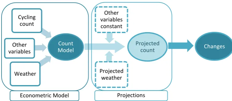
The basic modeling framework involves developing a bicycle count model for London using not only weather, but also other explanatory factors, and then employing this model to predict the level of future cycling by plugging in future projected weather data from climate simulations. Since future weather pattern is not deterministic in nature, we also run various plausible weather patterns consistent with the changed climate to quantify the plausible distribution of the potential changes in the cycling flow in the changed climate. The modeling framework is explained graphically in Fig. 1, and the key components are described below.

[Fig. 1 here]

3.2. Count Model Data

6 data is generally of good quality, some light bicycles may have been missing due to the loop nature of the automatic counters. The count information is available in hourly resolution from 6 am to midnight, while counts between midnight and 6 am are merged together. For modeling purpose these 6-hour long data was divided by 6 to get average hourly count. We used four years of data from January 1, 2008 to December 31, 2011 in this study. There are some gaps in the time series data in most of the counters, but they do not appear systematic. Also, given that we treat the temporal dimension using hourly, daily and monthly dummy variable during estimation, and do not use time series models explicitly, these random gaps do not affect our estimation process.

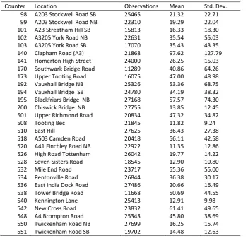
Some of the TLRN counters observe very few counts indicating a low cycling road. We remove from our sample those counters which register, on average, less than 10 cycles an hour during the 4 year period. We also remove any counter which has less than 18 months of data. This leaves us with 29 counters, and on average 22,465 observations, i.e. more than 3 years of observations, per counter. Summary information of these 29 counters is presented in Table 1.

[Table 1 here]

Hourly weather data on precipitation (mm), snowfall (mm), wind speed (knots/hour), relative humidity (%) and sunshine duration (hour) were collected from the British Atmospheric Data Centre's MIDAS database of the UK Meteorological Office (2013) for the nearest weather station to London, at Heathrow. Summary of this information is presented in Table 2. The hourly data is cleaned and matched with corresponding cycle count data. In order to incorporate non-linear response to some of these weather variables, dummy variables were created during the modelling process.

[Table 2 here]

3.3. Future Weather Data

7 km2 grids) and temporal resolutions for different emissions scenarios. Detail of UKCP 09 is available in DEFRA (2013).

GCMs like HadCM3 have coarser spatial, and particularly, temporal resolution than required for our research. We therefore use the weather generator application of the UKCP 09, which is described in detail in DEFRA (2013). In brief, the weather generator uses a downscaling process that produces synthetic hourly or daily time series for some of the weather variables which are consistent with the climate projections of the GCMs. The underlying modeling framework uses a stochastic rainfall process calibrated using past weather data and monthly climate projection data from HadCM3 to project future rainfall sequences on a daily basis. Mathematical relationships between rainfall and other weather variables, calibrated using past data, are then used to generate daily temperature range, relative humidity and sunshine hours. The hourly projections are then determined by disaggregating the daily data using observed hourly patterns and relationships to maintain the consistency between hourly and daily projections. Since the projected hourly and daily time series data are synthetic in nature, there are numerous plausible hourly and daily time series projections that are statistically equivalent to each other and are consistent with the HadCM3's probabilistic climate outputs. UKCP 09 weather generator therefore produces a large number (user-specified) of such representative weather simulations, each of which are consistent with the climate model projections under three emissions scenarios. 100 such projections of future weather variables under the high emissions scenario are used as inputs to our cycle count model to generate a distribution of future cycle counts in London network. Summary of these 100 simulations of the projected weather in year 2041 is presented in Table 2 above.

3.4. Count Model Methodology

We follow an econometric modelling approach to develop and estimate our base count model. Our dependent variable is an hourly time series (with gaps) of bicycle counts at different counter locations on TLRN. The explanatory variables are precipitation, temperature, relative humidity, wind speed, sunshine hours to capture the effects of weather, hourly, weekly and monthly dummy variables to capture the hourly, weekly and seasonal variations of the flow, and other dummy variables representing a step change in cycling conditions. Following the literature review, which indicates potential non-linear effects of precipitation, temperature and wind speed, we use several dummy variables representing different ranges of each of these three variables instead of using three continuous variables.

8 is the opening of the extensive Bike Hire system and two Cycling Superhighways in July 2010 (Transport for London 2012). It is therefore important to control for these factors. In addition, in order to represent the potential substitution relationships with other transport modes we include daily bus fares on Oyster Card (smart fare card), which changed in 2009 and 2011, as an explanatory factor. The nominal fares were converted to real fares using monthly consumer price index for London (ONS 2013a). The congestion charge into central London also changed from 3 January 2011, while the extent of congestion zone was reduced on 27 December 2010 - a dummy variable represents these events, too. Given the substantial recession in the UK during the 2008-2011 period and the importance of income on transport choices, we also include real wage rate and unemployment rate during the four years as control variables (ONS 2013b, Greater London Authority 2013).

Hourly bicycle count is a non-negative, discrete variable, which is often distributed as a Poisson or Negative Binomial distribution. Although we find a few log-linear OLS models in the literature, simple log-linear OLS models are not appropriate for count variables because the errors are non-normal and heteroskedastic, thereby making OLS estimates biased. (Cameron and Trivedi 1998). While at large mean expected hourly bicycle flows parameter estimates from a log-linear OLS and Poisson/Negative Binomial model may not be very different, standard errors and inference can still be quite different. The mean expected hourly flow is quite small in (<30) in many of our counters. Presence of valid zero counts in the data also makes OLS log-linear models troublesome. We therefore treat specifically the count nature of the dependent variable and use Poisson and Negative Binomial regression approach (and test which one is more appropriate).

Given our dataset is a time series for different counter locations, the dataset can be described as panel. However, our independent variables are the same across all counter locations, thus a traditional panel econometric approach does not improve our estimation. On the other hand, pooling the bicycle counts of all counters together is not appropriate either because of the large differences in flow in different counters. We therefore hypothesize that the differences between cycle flows among the counters are fixed in nature and include dummy variables for every counter. This approach is similar to a fixed effects panel model.

9 do not expect a similar change in one explanatory factor to have the same absolute effect on a low flow and a high flow location.

Within each day, the traffic flow varies depending on the hour. Preliminary graphical analysis reveals that the roads on which the counters are located show three distinct hourly traffic flow patterns: primarily morning peaks, primarily afternoon peaks and both peaks. Since the relationship between different hourly flows in a day is specific to each counter location, we allow the hourly patterns of daily cycle flow to vary between counters. We achieve this by interacting hourly dummy variable with dummy variables for counter locations. Similarly we allow for the weekly flow pattern to be distinct for each counter location by interacting the days of the week with counter locations. At the monthly level, which captures the seasonality in the time series, we use a common monthly dummy for all locations.

Given this background, our model has the following functional specification:

where, µit = mean hourly count at counter i (i =29) at time t

εit = errors

other lower case Greek letters = parameters to be estimated variables in capital = dummy variables (explained in Table 3)

variables in lower case = continuous variables (explained in Table 3)

As discussed earlier, the expected mean hourly cycle count, µ, has a Poisson or Negative Binomial distribution for our two model specifications. The underlying assumption in a Poisson distribution is that the mean is equal to the variance, whereas in Negative Binomial distribution this restriction is relaxed allowing for over dispersion of the data. Also, Poisson distribution is characterized by only one parameter, the mean, while Negative Binomial is characterized by the mean and a dispersion factor, which is estimated during the regression process. Both the Poisson and Negative Binomial regression models are estimated by the maximum likelihood method. The econometric details of the estimation methods are available in Cameron and Trivedi (1998).

log 𝜇𝑖𝑡 = 𝛼𝑖 𝐶𝑂𝑈𝑁𝑇𝐸𝑅𝑖 29

𝑖=1 + 𝛽𝑗 𝑅𝐴𝐼𝑁𝑗𝑡 4

𝑗 =2 + 𝜇 𝑅𝐴𝐼𝑁𝐿𝐴𝐺𝑡+ 𝛾𝑘 𝑇𝐸𝑀𝑃𝑘𝑡 4

𝑘=2

+ 𝛿_𝑙 4 𝑊𝐼𝑁𝐷_𝑙𝑡

𝑙=2 + 𝜃 𝐻𝑢𝑚𝑖𝑑𝑡+ 𝜌 𝑆𝑢𝑛𝑡+ 𝜏 𝑆𝑁𝑂𝑊𝑡+ 𝜑 𝑊𝑎𝑔𝑒𝑡+ 𝜔 𝑈𝑛𝑒𝑚𝑝𝑡

+ 𝜅 𝐵𝑢𝑠𝑓𝑎𝑟𝑒_𝑡+ 𝜆 𝐶𝑂𝑁𝐺𝐸𝑆𝑇_𝑡+ 𝜉 𝐼𝑁𝐹𝑅𝐴𝑆_𝑡+ 𝜐 𝑆𝑇𝑅𝐼𝐾𝐸_𝑡+ ώ 𝑆𝐻𝑂𝐿𝐼𝐷𝐴𝑌_𝑡

+ 𝜂𝑝 𝑀𝑂𝑁𝑇𝐻𝑝𝑡 12

𝑝=2 + 𝜁𝑖𝑚 𝐶𝑂𝑈𝑁𝑇𝐸𝑅𝑖𝑡𝐻𝑂𝑈𝑅𝑚𝑡 𝑖=29,𝑚=19

𝑖=1,𝑚=1

+ 𝜓_𝑖𝑛 𝑖=29,𝑛=5𝐶𝑂𝑈𝑁𝑇𝐸𝑅_𝑖𝑡𝐷𝐴𝑌_𝑛𝑡

10 Our literature review suggests that the sensitivity to rainfall, wind or temperature for commuting or utilitarian and recreational travel can be different. We hypothesize that weekday travel is generally utilitarian and weekend travel is for leisure and therefore run two separate models for weekdays and weekends to test if the parameter estimates are indeed different. We also include public (bank) holidays in the weekend model, specifically, as having the flow characteristics of a Sunday.

4. Results

4.1. Cycling Count Model

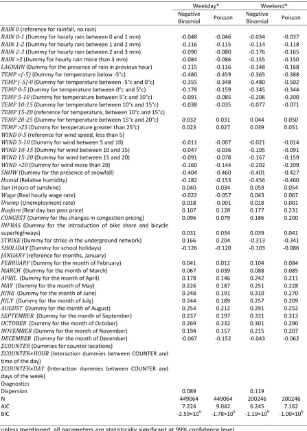
Estimation results for weekdays and weekends are presented in Table 3, for Negative Binomial and Poisson regression. The statistical test on the choice between a Negative Binomial and Poisson model hinges on the significance of the dispersion parameter in the Negative Binomial model: if it is different from zero, then Negative Binomial model is preferred. We indeed find that the dispersion parameter is statistically different from zero at 99% confidence level. Therefore we opt for the Negative Binomial model.

[Table 3 here]

We include the results for monthly dummies in the Table 3, but omit the parameter estimates for the dummy variables for individual counters and hourly and day of week interactions with counters for the sake of brevity (full parameter estimates are available on request). These parameters are plotted in Figs. 2 and 3 graphically. Three different patterns of hourly bicycle flows are highlighted (thick lines) for three representative counter locations in Fig. 2. Most of the locations show two peaks, but even among those there are substantial differences in the relative magnitudes, justifying our approach of interacting counter locations with hours.

[Fig. 2 here]

The differences between daily patterns in a week are not as large as the hourly differences (Fig. 3). Except for one counter (no. 173) all the counters show a similar non-linear daily cycle flow pattern: slight increases during Tuesdays and Wednesdays as compared to Mondays and then dropping off significantly on Fridays. Total daily flows during Saturdays and Sundays are even smaller (although they cannot be plotted on the same graph due to differences in the scale of two models), with Sundays and public holidays showing the smallest cycle flows (from weekend model results). Note that our model has a semi-logarithmic functional form, therefore the parameter estimates are not the traditional elasticities. Also, the parameter estimates between the counters cannot be used to directly compare the absolute flow characteristics between counters.

11 The weekday model supports previous assertion that rain adversely affects cycling flows, with maximum reduction taking place for hourly rains between 1 and 2 mm in our case. A substantial and statistically significant lagged effect of rain is also clearly visible. An increase in temperature increases bicycle usage, but the increase is non-linear and levels off (or slightly decreases) at temperatures above 25°c. Higher wind speed reduces cycling flows, with the effect nearly linear. Presence of snow has the largest impact on cycling, with a reduction of around 40% in weekday flows. An increase in humidity reduces bicycle use, while an increase in sunshine hours increases its use - although both effects are statistically significant, the absolute effects are not substantial.

A comparison of the weekday and weekend model reveals interesting insights. In general, the impact of weather is larger in the weekend model, which supports the hypothesis that leisure travel is more sensitive to weather events than utilitarian cycling. However, while this effect is pronounced at heavier rains, light rain does not deter leisure cycling more than utilitarian cycling. Effect of temperature is consistently larger for leisure cycling, with an aberration at very low temperatures (which is possibly spurious). Snow has similar effect on weekday and weekend cycling, but humidity has a substantially larger effect on weekend cycling flows.

During weekdays, an increase in the real wage rate reduces bicycle flows (2.18% for every GBP increase), hinting that utilitarian cycling could be an ‘inferior’ good, although this hypothesis requires further investigation using other measures of income. An increase in unemployment rate also increases cycling flow during weekdays by 1.82%. Cycling flows during weekdays in London increases substantially with an increase in bus fares (by 11.3% for every GBP increase), an increase in the congestion charge to central London (by 10% in January 2011 price hike) or a strike in the underground rail network (by 18.1% during strike days), all of which reveals cycling as a substantial substitute transport mode in London. The effects of wage rate, unemployment, bus fare and congestion charge together partially explain the increase in bicycle usage in London during 2008-2011 period. In comparison, the opening of the cycle hire and the two bicycle superhighways had a relatively modest association with the increase of bicycle flows (3.15% in July 2011), although the longer term impact, which would require a longer time series of data to investigate, could be larger. Also our time series is small (only 4 years) to decipher any longer term propensity toward increased cycling – therefore the parameter estimates for wage rate and unemployment should be treated with care, as they might reflect the effect of time too.

12 travel chaos a strike brings about, it is possible that people simply forego their leisure travel during the strike days generating the negative impact on weekend cycling.

4.2. Future Projected Cycling

4.2.1. Average effects

Projected future weather pattern under a changed climate scenario for 2041 is fed into the hourly bicycle count model to get projected bicycle count in 2041. Given some of the variables (snow, wind speed) are not available from the UKCP 09, these variables are kept at the base year values. We use year 2011 as our base year, which is the latest available data for our count model. However, instead of directly using 2011 cycle counts as our base dataset for comparison, we use predicted bicycle count from the econometric model for year 2011. We use the predictions for our baseline cycling counts in order to overcome the missing data in some of the counters. This results in an annual average hourly cycle count of 39.81 (95% confidence interval 39.58-40.04) in the TLRN network.

Given we have 100 simulations of future hourly weather patterns, we also have 100 projected hourly counts for each hour of the year. The annual average of these 100 mean hourly bicycle counts is 40, with 95% confidence interval between 39.98 and 40.02. This is a difference of only 0.5% from the baseline weather scenario of 2011, which is not statistically significant at 95% confidence (although significant at 90%). The primary reason for the relatively modest change is the counteracting effects of rain and temperature, as found by Bocker et al. (2013a) as well. A projected increase in temperature increases future bicycle use, but an increase in rainfall tempers the effect. Especially, 2011 was the driest and the warmest of the four years for which we have our cycle count data, therefore the projected changes were the smallest.

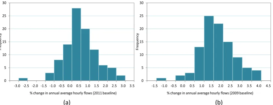
A further look into the annual average bicycle count for each plausible weather pattern shows a range of an increase of 2.6% to a reduction of 2.5%. Around 20% of the plausible weather patterns result in a possible reduction in flow, albeit most of it marginal. Fig. 4(a) presents the frequency distribution of the changes in annual average hourly cycle flows for the 100 plausible future weather patterns.

[Fig. 4 here]

13 38.84 per hour on average, indicating a 1.7% increase, which is statistically significant as well.1 Fig. 4(b) presents the distribution of changes for this case, which shows larger increases than Fig 4(a). The frequency distribution also shows that in only 3 cases there were no increases in cycling flows in 2041 with respect to the flow in 2009; and the range of change varies from -1.3% to +3.9%.

4.2.2. Seasonal and weekly effects

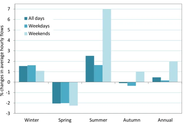
The changes in the weather pattern due to climate change are not constant throughout all seasons. Since the weather patterns during different seasons get affected differently, the seasonal changes in the cycle flows are also expected to be different in a changed climate. The fine temporal resolution in our count modelling framework easily allows us to decipher the differences in seasonal changes in the cycling flows due to climate change. Modelling results show that cycling flows increase by 1.5% in the winter and 2.5% during the summer over year 2011 baseline (Fig. 5). However, these increases are countered by a reduction of 2.0% and 0.1% during the spring and autumn respectively, resulting in a net annual hourly increase of 0.5%, as mentioned earlier.

[Fig. 5 here]

Disaggregating the seasonal patterns further into weekdays (representing utilitarian cycling) and weekends (representing leisure cycling), we again find differential impacts. During the winter, weekday bicycle counts increase more than the weekend bicycle counts (1.61% to 1.1%). The differences between the climate induced changes in cycling flows during the weekends and weekdays is the least prominent during the spring, when they are reduced by 2.25% and 2% respectively. On the other hand, the Summer months show a large variation: weekday flows increase by 1.6%, but weekend (and holidays) flows increase by 7%. During the autumn, weekday flows show a slight reduction (0.35%) but weekend flows increase by 1%, with a negligible change in the combined impact. On an annual hourly average basis, weekday bicycle flows increase by only 0.17%, while weekend flows increase by 1.97%. All of these seasonal and weekly changes are calculated on the basis of a 2011 baseline, and a 2009 baseline would most likely show even larger increases.

5. Conclusions

The use of bicycle as a transport mode or a leisure activity is particularly affected by the different elements of daily weather, which is expected to change considerably in the future because of the climate change. The objective of this paper was to develop a framework that could be used to determine the impact of climate induced changes in future weather pattern on bicycle flows and apply that framework to London which has seen a rapid growth in cycling in the past decade. We

1 _{The difference in 2041 flows for the two baseline scenarios of 2009 and 2011 is due to the differences in the}

14 developed a bicycle count model for London and employed the UKCP 09 modelling results for future climate change to understand the potential changes in bicycle flow in 2041, with respect to those in 2011. To our knowledge, this is the first study to utilize an hourly resolution future weather data, downscaled from the GCMs, to study the effect of climate change on bicycle use. In order to capture the potential uncertainty in future climate change and the associated weather patterns, we also simulate 100 plausible weather patterns under a changed climate, which is a different approach from the existing studies which use single values for the annual changes in the weather. Our bicycle count model for London supports previous findings that bicycle flow is indeed sensitive to the weather, with leisure cycling more sensitive than the utilitarian one. We also found evidence that utilitarian cycling could decrease as a result of higher income or lower unemployment rate which could potentially lead to lower cycling for commuting when the UK economy gains momentum in the future.

Bicycle flow in London is expected to increase due to the climate change, although the magnitude of this increase is modest, even in the high emissions scenario of UKCP 09. Given the high temporal resolution of our count model, the projected relative changes in future bicycle flows are sensitive to the choice of the baseline year. By 2041, bicycle flows are expected to increase during the summer and the winter, but the reductions in the spring and the autumn temper the net annual effect. The largest increase (~7% over year 2011 baseline) in bicycle use is during the weekends of the summer months for leisure travel. This would potentially result in better utilization efficiency of the bicycle infrastructure during the summer off-peak periods. The maximum increase in daily weekday travel is 1.6% during the summer and the winter, which is not very large. Still, even this small increase can be important if the future bicycle network gets congested - a possibility during the summer months - as it can result in a more than proportional increase in travel delay.

Care must be exercised in interpreting our results. Longer run cycling flows depend on a number of other, possibly more influencing variables than weather, e.g. policy and safety initiatives, new technologies or prices of fuel and alternate transport modes, etc. Also there could be substantial changes in the perception about cycling and related behavioural traits over the next few decades. Our model thus is more appropriate in answering the question what happens if we have a changed weather pattern due to climate change now, rather than what happens in general in the future. Nonetheless, the relative impacts on cycle flows from our model will remain valid as long as people's sensitivity to the weather variables do not change, although the absolute flow levels may not.

15 increases in the bicycle flow. Although we could not incorporate changes in wind speed too, recent results of UKCP 09 show that future changes in wind speed and thus its effect on our results is negligible. Our model also does not incorporate the impacts of extreme weather induced events, e.g. bike path or bike lane closures due to flooding resulting from excessive rainfall, which can be important for climate adaptation planning. This would require a different modelling approach, possibly in the area of asset management. Also, our results cannot be generalized to every other region in the world since the changes in weather pattern due to a changed climate and the sensitivity of bicycle use to temperature and rainfall will be different spatially. However, the modeling framework can be applied universally subject to the availability of the underlying data.

Acknowledgements

The author thanks Transport for London (TfL) for providing the data from the automated bicycle counters for London.

References

Ahmed F, Rose G and Jacob C 2010. Impact of weather on commuter cyclist behaviour and implications for

climate change adaptation, 33rd Australasian Transport Research Forum, Canberra

Ahmed F, Rose G, Figliozzi M and Jakob C 2012. Commuter cyclists sensitivity to changes in weather: Insights

from two cities with different climatic conditions, 91st Annual Meeting of the Transportation Research

Board, Jan, Washington DC

Bergstrom A and Magnussen R 2003. Potential of transferring car trips to bicycle during winter, Transportation

Research Part A, Vol. 37, pp. 649-666

Bocker L, Dijst M and Prillwitz J 2013b. Impact of everyday weather on individual daily travel behaviours in

perspective: A literature review, Transport Reviews, Vol. 33, No. 1, pp. 71-91

Bocker L, Prillwitz J and Dijst M 2013a. Climate change impacts on mode choices and travelled distance: A

comparison of present with 2050 weather conditions for the Randstad Holland, Journal of Transport

Geography, Vol. 28, pp. 176-185

Brandenburg C, Matzarakis A and Arnberger A 2007. Weather and cycling – A first approach to the effects of

weather condition on cycling, Meteorological Applications, 14, 61-67

Buehler R and Pucher J 2012. Cycling to work in 90 large American cities: new evidence on the role of bike

paths and lanes, Transportation, Vol. 39, pp. 409-432

Cameron AC and Trivedi PK 1998. Regression analysis of count data, Cambridge University Press, Cambridge

Cervero R and Duncan M 2003. Walking, bicycling and urban landscapes: Evidence from the San Francisco Bay

Area, American Journal of Public Health, Vol. 93, No. 9, pp. 1478-1483

DEFRA (Department for Environment, Forrest and Rural Affairs) 2013 [online]. UK Climate Impact Project 2009,

16 Dill J and Carr T 2003. Bicycle commuting and facilities in Major US cities: If you build them, commuters will use

them - Another look, 82nd Annual Meeting of the Transportation Research Board, Washington DC

ECF (European Cyclists' Federation) 2011. Cycle more often 2 cool down the planet: Quantifying CO2 savings of

cycling, Brussels

Emmerson P, Ryley TJ and Davies DG 1998. The impact of weather on cycle flows, Traffic Engineering and

Control, April

Flynn BS, Dana GS, Sears J and Aultman-Hall L 2012. Weather factor impacts on commuting to work by bicycle,

Preventive Medicine, Vol. 54, pp. 122-124

Gebhart K and Noland RB 2013. The impact of weather conditions on capital bikeshare trips, 92nd Annual

Meeting of the Transportation Research Board, Jan 13-17, Washington DC

Goetzke F and Rave T 2011. Bicycle use in Germany: Explaining differences between municipalities through

network effects, Urban Studies, Vol. 48, No. 2, pp. 427-437

Greater London Authority 2013 [online]. Unemployment rate, region, available at:

http://data.london.gov.uk/datastore/package/unemployment-rate-region, accessed: 17 May 2013

Hanson S and Hanson P 1977. Effects of weather on bicycle travel, Transportation Research Record, No. 629,

pp. 43-48

Heinen E, Maat K and van Wee B 2011. Day-to-day choice to commute or not by bicycle, Transportation

Research Record: Journal of the Transportation Research Board, No. 2230, pp. 9-18

Keay C 1992. Weather to cycle, Ausbike 92: Proceedings of a national bicycle conference, pp. 152-155,

Melbourne

Koetse MJ and Rietveld P 2009. The impact of climate change and weather on transport: An overview of

empirical findings, Transportation Research Part D, Vol. 14, pp. 205-221

Lathia N, Ahmed S and Capra L 2012. Measuring the impact of opening the London shared bicycle scheme to

casual users, Transportation Research Part C, Vol. 22, pp. 88-102

Miranda-Moreno LF and Nosal T 2011. Weather or not to cycle: Temporal trends and impact of weather on

cycling in an urban environment, Transportation Research Record: Journal of the Transportation Research

Board, No. 2247, pp. 42-52

Nankervis M 1999. The effect of weather and climate on bicycle commuting, Transportation Research Part A,

Vol. 33, pp. 417-431

ONS (Office for National Statistics) 2013a [online]. Consumer Price Indices time series data table, available at:

http://www.ons.gov.uk/ons/rel/cpi/consumer-price-indices/april-2013/cpi-time-series-data.html, accessed:

1 May 2013

ONS (Office for National Statistics) 2013b [online]. Regional Economic Analysis, Changes in real earnings in the

UK and London, 2002 to 2012, available at:

http://www.ons.gov.uk/ons/rel/regional-trends/regional-economic-analysis/changes-in-real-earnings-in-the-uk-and-london--2002-to-2012/index.html, accessed 1

May 2013

Parkin J, Wardman M and Page M 2008. Estimation of the determinants of bicycle mode share for journey to

17 Phung J and Rose G 2007. Temporal variations in usage of Melbourne's bike paths, 30th Australasian Transport

Research Forum, Melbourne

Pooley C, Horton D, Scheldman G, Tight M, Harwatt H, Jopson A, Jones T, Chisholm A and Mullen C 2010. Can

increased walking and cycling really contribute to the reduction of transport-related carbon emissions?

Royal Geographical Society Annual Conference, London

Pooley C, Tight M, Jones T, Horton D, Scheldeman G, Jopson A, Mullen C, Chisholm A, Strano E and Constantine

S 2011. Understanding walking and cycling: Summary of key findings and recommendations, Lancaster

University

Pucher J and Buehler R 2006. Why Canadians cycle more than Americans: A comparative analysis of bicycling

trends and policies, Transport Policy, Vol. 13, pp. 265-279

Rashad I 2009. Associations of cycling with urban sprawl and the gasoline price, American Journal of Health

Promotion, Vol. 24, No. 1, pp. 27-36

Richardson AJ 2000. Seasonal and weather impacts of urban cycling trips, TUTI Report 1-2000, The Urban

Transport Institute, Victoria

Sabir M 2011. Weather and travel behaviour, PhD Dissertation, Vrije Universiteit, Amsterdam

Saneinejad S, Roorda MJ and Kennedy C 2012. Modelling the impact of weather conditions on active

transportation travel behaviour, Transportation Research Part D, Vol. 17, pp. 129-137

Smith MS and Kauermann G 2011. Bicycle commuting in Melbourne during the 2000s energy crisis: A

semiparametric analysis of intraday volumes, Transportation Research Part B, Vol. 45, pp. 1846-1862

Thomas T, Jarsma R and Tutert 2013. Exploring temporal fluctuations of daily cycling demand on Dutch cycle

paths: the influence of weather on cycling, Transportation, Vol. 40, pp. 1-22

Tin ST, Woodward A, Robinson E and Ameratunga S 2012. Temporal, seasonal and weather effects on cycle

volume: an ecological study, Environmental Health, Vol. 11, No. 12, pp. 1-9

Transport for London 2012 [online]. Transport for London's written submission to the London Assembly

Transport Committee's investigation into cycling in London, available at:

http://www.london.gov.uk/sites/default/files/TfL-Written-Submissions-cycle-evidence.pdf, accessed: 11 May

2013

UK Government 2013 [online]. Policy: Adapting to climate change, available at:

https://www.gov.uk/government/policies/adapting-to-climate-change, accessed 25 May 2013

UK Meteorological Office 2011. Climate: Observations, projections and impacts, crown copyright

UK Meteorological Office 2013 [online]. Met Office Integrated Data Archive System (MIDAS) Land and Marine

Surface Stations Data (1853-current). NCAS British Atmospheric Data Centre, Available from

http://badc.nerc.ac.uk/view/badc.nerc.ac.uk__ATOM__dataent_ukmo-midas, accessed: 3 Jan 2013

UK Parliament 2013 [online]. Daily Hansard- Written Answers, 15 June 2011, available at:

http://www.publications.parliament.uk/pa/cm201011/cmhansrd/cm110615/text/110615w0002.htm#11061

561000164, accessed 31 March 2013

18 Wardman M, Tight M and Page M 2007. Factors influencing the propensity to cycle to work, Transportation

Research Part A, 41, 339-350

Winters M, Friesen MC, Koehoorn M and Teschke 2007. Utilitarian bicycling: A multilevel analysis of climate

and personal influences, American Journal of Preventive Medicine, Vol. 32, pp. 52-58

19

Cycling in a Changed Climate

Figures

Fig. 1 Modeling framework

Fig. 2 Estimates for hourly flow dummies (ζim) for different counters

0 1 2 3 4 5

5 6 7 8 9 10 11 12 13 14 15 16 17 18 19 20 21 22 23

Pa

ra

m

ete

r

es

ti

m

ate

Start time for the hour of the day

99 101 103 140 141 173 192 194 195 200 501 508 510 518 520 526 528 532 534 536 538 540 542 548 550 551 98 102 170

Projected count

Projected weather

Other variables constant

Count Model

Weather Other variables

Cycling count

Changes

20 Fig. 3 Estimates for days of the week (weekdays) dummies (ψin) for different counters

(a) (b)

Fig. 4 Distribution of changes in bicycle flows for 100 plausible weather patterns in 2041, with respect to (a) 2011 and (b) 2009 baseline

-0.20 -0.15 -0.10 -0.05 0.00 0.05 0.10 0.15

Mon Tues Wed Thurs Fri

Par am ete r es ti m ate

Day of week

98 99 101 102 103 140 141 170 173 192 194 195 200 501 508 510 518 520 526 528 532 534 536 538 540 542 548 550 551

0 5 10 15 20 25 30 Fr e q u e n cy

% change in annual average hourly flows (2011 baseline)

0 5 10 15 20 25 30 Fr e q u e n cy

21 Fig. 5 Percent change in bicycle flows due to climate change during weekdays and weekends for different seasons

-3 -2 -1 0 1 2 3 4 5 6 7

Winter Spring Summer Autumn Annual

%

c

h

an

ge

s

in

av

er

ag

e

h

o

u

rl

y

fl

o

w

s

22

Cycling in a Changed Climate

Tables

Table 1. Summary of bicycle count data of 29 TLRN counters

Counter Location Observations Mean Std. Dev. 98 A203 Stockwell Road SB 25465 21.32 22.71 99 A203 Stockwell Road NB 22310 19.29 22.04 101 A23 Streatham Hill SB 15813 16.33 18.30 102 A3205 York Road NB 22631 35.54 55.03 103 A3205 York Road SB 17070 35.43 43.35 140 Clapham Road (A3) 21868 97.62 127.79 141 Homerton High Street 24000 26.25 15.03 170 Southwark Bridge Road 11289 40.86 64.26 173 Upper Tooting Road 16075 47.00 48.98 192 Vauxhall Bridge NB 25326 53.36 68.75 194 Vauxhall Bridge SB 24780 34.19 38.32 195 Blackfriars Bridge NB 27168 57.57 74.30 200 Chiswick Bridge NB 27755 13.85 12.45 501 Upper Richmond Road 20834 47.32 34.82

508 Tooting Bec 21845 11.82 9.24

510 East Hill 27625 36.43 27.38

518 A503 Camden Road 20418 56.11 42.58 520 A41 Finchley Road NB 22922 11.35 12.86 526 High Road Tottenham 26042 19.77 14.22 528 Seven Sisters Road 18545 12.90 10.80 532 Mile End Road 23717 55.36 55.00 534 Pentonville Road 26844 36.38 30.17 536 East India Dock Road 27486 20.66 16.49 538 Tower Bridge Road 11668 50.69 44.55 540 Kennington Lane 25413 12.91 9.98 542 New Cross Road 23832 61.41 49.65 548 A4 Brompton Road 25343 45.80 38.69 550 Twickenham Road NB 27699 16.25 15.74 551 Twickenham Road SB 19702 14.48 12.63

Table 2. Summary of past and projected hourly weather information

Temperature (°c) Rainfall (mm/hr) Rainfall (hours) Snowfall (hours)* Wind speed (knot/hour)* Relative Humidity (%) Sunshine (hour) 2011

Spring (Mar-May) 11.74 0.0184 57 0 7.90 0.681 0.255

Summer (Jun-Aug) 16.52 0.0882 210 0 7.67 0.704 0.222

Autumn (Sep-Nov) 13.49 0.0348 107 0 8.53 0.799 0.162

Winter (Dec-Feb) 6.52 0.0839 231 0 9.23 0.834 0.061

2041

Spring (Mar-May) 12.31 0.0676 235 0 7.90 0.717 0.206

Summer (Jun-Aug) 18.77 0.0690 151 0 7.67 0.689 0.287

Autumn (Sep-Nov) 14.94 0.0850 227 0 8.53 0.789 0.144

Winter (Dec-Feb) 7.51 0.0765 272 0 9.23 0.832 0.070

23 Table 3. Parameter estimates for key explanatory factors

Weekday* Weekend*

Negative

Binomial Poisson

Negative

Binomial Poisson RAIN 0 (reference for rainfall, no rain)

RAIN 0-1 (Dummy for hourly rain between 0 and 1 mm) -0.048 -0.046 -0.034 -0.037

RAIN 1-2 (Dummy for hourly rain between 1 and 2 mm) -0.116 -0.115 -0.114 -0.118

RAIN 2-3 (Dummy for hourly rain between 2 and 3 mm) -0.090 -0.080 -0.176 -0.165

RAIN >3 (Dummy for hourly rain more than 3 mm) -0.084 -0.086 -0.155 -0.150

LAGRAIN (Dummy for the presence of rain in previous hour) -0.115 -0.116 -0.148 -0.168

TEMP <(-5) (Dummy for temperature below -5°c) -0.480 -0.459 -0.365 -0.388

TEMP (-5)-0 (Dummy for temperature between -5°c and 0°c) -0.355 -0.348 -0.480 -0.502

TEMP 0-5 (Dummy for temperature between 0°c and 5°c) -0.178 -0.159 -0.345 -0.344

TEMP 5-10 (Dummy for temperature between 5°c and 10°c) -0.091 -0.085 -0.206 -0.200

TEMP 10-15 (Dummy for temperature between 10°c and 15°c) -0.038 -0.035 -0.077 -0.071

TEMP 15-20 (reference for temperature, between 10°c and 15°c)

TEMP 20-25 (Dummy for temperature between 15°c and 20°c) 0.032 0.031 0.044 0.050

TEMP >25 (Dummy for temperature greater than 25°c) 0.023 0.027 0.039 0.051

WIND 0-5 (reference for wind speed, less than 5)

WIND 5-10 (Dummy for wind between 5 and 10) -0.011 -0.007 -0.021 -0.014

WIND 10-15 (Dummy for wind between 10 and 15) -0.047 -0.036 -0.105 -0.091

WIND 15-20 (Dummy for wind between 15 and 20) -0.091 -0.078 -0.167 -0.159

WIND >20 (Dummy for wind more than 20) -0.160 -0.144 -0.202 -0.209

SNOW (Dummy for the presence of snowfall) -0.404 -0.460 -0.401 -0.427

Humid (Relative humidity) -0.182 -0.153 -0.456 -0.460

Sun (Hours of sunshine) 0.040 0.034 0.059 0.054

Wage (Real hourly wage rate) -0.022 -0.057 0.043 0.067

Unemp (Unemployment rate) 0.018 -0.001 0.018 0.001

Busfare (Real day bus pass price) 0.107 0.128 0.177 0.231

CONGEST (Dummy for the changes in congestion pricing) 0.096 0.079 0.186 0.200

INFRAS (Dummy for the introduction of bike share and bicycle

superhighways) 0.031 0.034 0.039 0.041

STRIKE (Dummy for strike in the underground network) 0.166 0.204 -0.313 -0.341

SHOLIDAY (Dummy for school holidays) -0.126 -0.120 -0.103 -0.086

JANUARY (reference for months, January)

FEBRUARY (Dummy for the month of February) 0.041 0.012 0.104 0.084

MARCH (Dummy for the month of March) 0.067 0.039 0.088 0.085

APRIL (Dummy for the month of April) 0.178 0.146 0.242 0.211

MAY (Dummy for the month of May) 0.226 0.187 0.251 0.228 JUNE (Dummy for the month of June) 0.248 0.191 0.310 0.270 JULY (Dummy for the month of July) 0.244 0.189 0.257 0.209

AUGUST (Dummy for the month of August) 0.254 0.212 0.291 0.252

SEPTEMBER (Dummy for the month of September) 0.237 0.197 0.331 0.313

OCTOBER (Dummy for the month of October) 0.269 0.232 0.301 0.290

NOVEMBER (Dummy for the month of November) 0.194 0.157 0.215 0.207

DECEMBER (Dummy for the month of December) -0.067 -0.152 -0.043 -0.062

ΣCOUNTER (Dummies for counter locations)

ΣCOUNTER×HOUR (Interaction dummies between COUNTER and time of the day)

ΣCOUNTER×DAY (Interaction dummies between COUNTER and days of the week)

Diagnostics

Dispersion 0.089 0.119

N 449064 449064 200246 200246

AIC 7.224 9.042 6.245 7.162

BIC -2.59×106 -1.78×106 -1.19×106 -1.00×106