A Programmable look-up table-based interpolator with nonuniform sampling scheme

nonuniform sampling scheme

.

White Rose Research Online URL for this paper:

http://eprints.whiterose.ac.uk/75065/

Version: Published Version

Article:

Dutra e Silva Junior, Elvio Carlos, Soares Indrusiak, Leandro

orcid.org/0000-0002-9938-2920, Finamore, W.A. et al. (1 more author) (2012) A

Programmable look-up table-based interpolator with nonuniform sampling scheme.

International Journal of Reconfigurable Computing. 647805. ISSN 1687-7209

https://doi.org/10.1155/2012/647805

[email protected] https://eprints.whiterose.ac.uk/

Reuse

Items deposited in White Rose Research Online are protected by copyright, with all rights reserved unless indicated otherwise. They may be downloaded and/or printed for private study, or other acts as permitted by national copyright laws. The publisher or other rights holders may allow further reproduction and re-use of the full text version. This is indicated by the licence information on the White Rose Research Online record for the item.

Takedown

If you consider content in White Rose Research Online to be in breach of UK law, please notify us by

Volume 2012, Article ID 647805,14pages doi:10.1155/2012/647805

Research Article

A Programmable Look-Up Table-Based Interpolator

with Nonuniform Sampling Scheme

´Elvio Carlos Dutra e Silva J ´unior,

_{Leandro Soares Indrusiak,}

Weiler Alves Finamore,

_{and Manfred Glesner}

1_{Department of Aerospace Science and Technology, Institute for Advanced Studies, 12228-001 S˜ao Jos´e dos Campos, SP, Brazil} 2_{Department of Computer Science, University of York, York YO10 5GH, UK}

3_{Department of Eletrical Energy, Federal University of Juiz de Fora, 36036-900 Juiz de Fora, MG, Brazil} 4_{Department of Microelectronic Systems, Darmstadt University of Technology, 64283 Darmstadt, Germany}

Correspondence should be addressed to ´Elvio Carlos Dutra e Silva J ´unior,[email protected]

Received 14 June 2012; Accepted 4 September 2012

Academic Editor: Scott Hauck

Copyright © 2012 ´Elvio Carlos Dutra e Silva J ´unior et al. This is an open access article distributed under the Creative Commons Attribution License, which permits unrestricted use, distribution, and reproduction in any medium, provided the original work is properly cited.

Interpolation is a useful technique for storage of complex functions on limited memory space: some few sampling values are stored on a memory bank, and the function values in between are calculated by interpolation. This paper presents a programmable Look-Up Table-based interpolator, which uses a reconfigurable nonuniform sampling scheme: the sampled points are not uniformly spaced. Their distribution can also be reconfigured to minimize the approximation error on specific portions of the interpolated function’s domain. Switching from one set of configuration parameters to another set, selected on the fly from a variety of precomputed parameters, and using different sampling schemes allow for the interpolation of a plethora of functions, achieving memory saving and minimum approximation error. As a study case, the proposed interpolator was used as the core of a programmable noise generator—output signals drawn from different Probability Density Functions were produced for testing FPGA implementations of chaotic encryption algorithms. As a result of the proposed method, the interpolation of a specific transformation function on a Gaussian noise generator reduced the memory usage to 2.71% when compared to the traditional uniform sampling scheme method, while keeping the approximation error below a threshold equal to 0.000030518.

1. Introduction

Nowadays, the world is facing a boom on the fusion between telecommunications and information technology. The merging of these two fields spreads over all kinds of information systems, requiring efforts for ensuring the inte-gration among many kinds of organizations [1], from tactical to strategic operations, in di_fferent levels of information system interoperability [2]. The ISO/OSI seven-layer model arises as a lighthouse for seeking the interoperability on many different layers of networked solutions [3]. Many standards and protocols arise from this model, including cryptographic ones.

Encryption solutions can be implemented on both software and hardware. Software implementations are more related to the protection of the information itself, while

hardware ones can be also used to protect the communi-cation channels [4]. In the case of tactical telecommunica-tion systems, which require both channel and informatelecommunica-tion security, the hardware implementation of such encryption algorithms arises as a better compromise. The need to test the behavior of such systems against different sources of noise and jamming becomes the motivation to implement, on FPGA (Field-Programmable Gate Array), a programmable noise generator.

common microelectronic blocks for many applications [5–

19]. Ba et al. [9] proposed a linearly interpolated LUT pre-distorter used to mitigate the effects of nonlinear amplifiers. Monga and Bala [10] proposed an algorithm for minimizing the approximation error on multidimensional LUTs where both samples values and distributions are optimized.

Some authors used nonuniform sampling schemes as a solution for minimizing the LUT memory size: Seidner [11] reduced the memory usage on the implementation of a 10Y conversion circuit with a LUT scaling sample scheme; Yan and M¨ammel¨a [15] used a nonuniformly segmented interpo-lation LUT for simulating nonlinear radio frequency power amplifiers; Cavers [16] proposed a systematic way to describe and analyze arbitrary nonuniform LUT sampling schemes as a companding function, which was further improved by Hassani and Kamarei [17] with a LUT segmentation concept; Boumaiza et al. [18] proposed a new companding function for amplifier predistortion with built-in dependence on the nonlinearity of the power amplifier; Dutra et al. [19] used a nonuniform but fixed sampling scheme to minimize the memory size of a LUT-based interpolator designed to represent the Inverse Error Function (erf−1).

All works previously mentioned used a fixed, uniform or not, sampling scheme to characterize a given function or class of functions. The main contribution of this work is to implement on FPGA a LUT-based interpolator system with a sampling scheme that isnot-fixed(it can be programmed on the fly) andnot-uniformlydistributed (it uses not equally spaced sampling points).

The remaining of the paper is organized as follows: based on the definition of partitions, Section 2 will present the offline calculations performed to define the parameters that configure the proposed programmable LUT-based interpo-lator. Section 3 will describe the interpolator architecture, including the description of the subsystem that calculates the nonuniformly distributed addresses and the corresponding displacements. An application of the proposed interpolator will be presented on Section 4, where its flexibility will be discussed with the usage of a gamma of different functions

g(x), using differentnot-fixedandnot-uniformlydistributed sampling schemes. Section 5 will end this paper with a summary of the achieved results and a flavor of future works.

2. Configuration Parameters

To discuss the determination of the configuration tables for the LUT-based interpolator, discussed hitherto, we will consider a generic function g(x) which will have notable values stored on the appropriate tables. To set an example, values that define a set of arbitrary intervals are stored in

Table 1. The number of intervals is related to the number of resources used on the FPGA implementation. As a project decision,P =22 partitions were used in order to minimize the final approximation error. Although we focus on a specific example, the underlined method is revealed in its generality.

To define the configuration tables for the LUT-based interpolator, we will consider a generic function g(x)

Table_{1: Frequency assignment for sampling schemeα.}

n xn fn

1 −1.00000000000000 32768

2 −0.99770000000000 16384

3 −0.99540000000000 8192

4 −0.99030000000000 4096

5 −0.98050000000000 2048

6 −0.95900000000000 1024

7 −0.91410000000000 512

8 −0.82040000000000 256

9 −0.64070000000000 128

10 −0.34380000000000 64

11 −0.12510000000000 32

12 +0.00000000000000 32

13 +0.12490000000000 64

14 +0.34360000000000 128

15 +0.64050000000000 256

16 +0.82020000000000 512

17 +0.91400000000000 1024

18 +0.95890000000000 2048

19 +0.98040000000000 4096

20 +0.99010000000000 8192

21 +0.99530000000000 16384

22 +0.99760000000000 32768

— +0.99993896484375 —

which will have only notable values stored on appropriate tables. We start by considering the interval [x1,xP+1) to be the

functiong(x) domain and a set of points_{x1,x2,. . .,xn,xn+1, . . .,xP,xP+1}which will induce thePpartitions{[x1,x2),. . .

, [xn,xn+1),. . ., [xP,xP+1)}on the domain [x1,xP+1). Samples

are next drawn from each element of partition [xn,xn+1),

where n ∈ {1, 2,. . .,P}, with a given frequency fn—the set of in = (xn+1 − xn)fn sampling points induces the subpartition{[xn1,xn2), [xn2,xn3),. . ., [xnin,xnin+1)}of thenth interval (notice that xn1 = xn and xnin+1 = xn+1). For each function g(x), the appropriate configuration table is stored—the values stored on the table contain, among other parameters discussed in this section, both the ordinate values given by the set{g(xn1),g(xn2),. . .,g(xnin+1)}and the corresponding derivate values {g′_(x

n1),g′(xn2),. . .,g′(xnin)}

estimated by (1), wherem∈ {1, 2,. . .,in}. Both ordinate and derivate values are defined forn∈ {1, 2,. . .,P}:

g′

xnm

=g

xnm+1

−g

xnm

xnm+1−xnm

. (1)

interval (x4,x5] = (−0.9903,−0.9805], with a sampling

frequency fn = 4096. Note also in Table 1 that xP+1 =

0.99993896484375.

The interval and sampling frequency of each partition should be chosen in order to allow the representation of g(x) with a minimum approximation error. Therefore, higher sampling frequencies fn should be expected on n intervals where g(x) changes more abruptly, presenting higher curvature. Based on the data ofTable 1, we calculate the configuration parameters of the LUT-based interpolator, as illustrated inTable 2and explained ahead.

We start the construction of Table 2 by adjusting the partitions limits_{x1,x2,. . .,xn,xn+1,. . .,xP,xP+1}ofTable 1

according to the sampling frequency of each partition. The Precise Inferior Limit (PIL) and the Corrected Superior Limit (CSL) of each partition n are calculated by (2) and (3) which use a constant binary decimal point position (d = 14), the function signal Sg(a), which outputs the values−1 or +1 according to the signal negative or positive of a given argument a (notice that for a null argument, Sg(0)=0), and the function roundR(b/c), which calculates the maximum multiple of the argumentc, less or equal to them the argumentb (note that the symbol / used on the representation of the function roundR(b/c) has no relation to the division operation). Both PIL and CSL are necessary for adjusting thenpartitions ofTable 1(an empiric project choice) to the corresponding frequencies:

PIL1=R

x1

Sg(x1)×21−log2(f1)

PILn=R ⎛

⎝

Rxn/Sg(xn)×21−log2(fn−1) Sg(xn)×21−log2(fn)

⎞

⎠,

(2)

CSLn=R ⎛

⎝

Rxn+1/Sg(xn+1)×21−log2(fn)

Sg(xn+1)×21−log2(fn+1) ⎞

⎠−2−d. (3)

Table 2also brings three parameters used to select some input bits of the LUT, necessary to calculate the addresses and di_fferences. They are the parameter Bn, calculated by (4) and used to select theBn more significant bits (MSBs) of input x, required on the calculation of the nonuniform spaced addresses; the parameterDn, calculated by (5) and used to slice the Dn less significant bits (LSBs) of inputx, also required on the addresses calculation; and parameter

Sn, calculated by (6) and used to slice theSnless significant bits (LSBs) of input x, required to calculate the difference (x−xnm) between the LUT input and the corresponding

stored sampling point. The usage of these parameters will be discussed inSection 3:

Bn=1−log₂fn, (4)

Dn=log2

fn, (5)

Sn=15−log2

fn, for fn=/215

Sn=7, for fn=215.

(6)

Two other important configuration parameters present inTable 2are the Displacement (Dsp_n) and the Address Logic (Add log_n), calculated by (7) and (8). These two parameters are used in the calculation of nonuniform spaced addresses, as will be presented in more details inSection 3:

Dsp_n= fn

2, (7)

Add log_n=SMNn−IMNn

SMNn=1 + EMNn−1

SMN1=0

EMNn=SMNn+ QMRn−1

QMRn=0.5×fn×

CSLn−PILn+ 2−d

IMNn=MNMn+ SMPn

MNMn=0.5×fn

SMPn=0.5×fn×PILn.

(8)

The quantities QMR, SMN, EMN, MNM, SMP, and IMN are intermediate variables necessary for the recursive calcula-tion of the Address Logic in (8). They are related, respectively, to the following entities: the Quantity of Memories Required (QMR) on each partitionn, the Starting Memory Number (SMN) and the Ending Memory Number (EMN) on each partition n, the Maximum Number of Memories (MNM) considering that the specific sampling frequency was applied to the entire domain [x1,xP+1), the Starting Memory Position

(SMP) considering that the specific sampling frequency was applied to the entire domain [x1,xP+1), and the Initial

Memory Number (IMN) used on the specific sampling frequency.

The last four configuration parameters are related to the calculation of the sampling points xnm used to define the

ordinate g(xnm) and derivate g′(xnm) stored values. These

parameters are the Sampling Points Start (SPS), Sampling Points Final (SPF), Memory Position Start (MPS), and the Memory Position Final (MPF), calculated by (9), (10), (11), and (12), respectively:

SPS1=PIL1

SPSn= 2

fn

+ SPFn−1,

(9)

SPF1=CSL1+ 2−d

SPFn=CSLn+ 2−d− 2

fn

, (10)

MPS1=1

MPSn=1 + MPFn−1,

Table_{2: Configuration parameters calculated for sampling schemeα.}

n PILn CSLn Bn Dn Sn Dspn Add logn SPSn MPSn SPFn MPFn

1 −1.00000000000 −0.99774169921 −14 15 7 16384 0 −1.00000000000 1 −0.99768066406 39

2 −0.99768066406 −0.99542236328 −13 14 1 8192 19 −0.99755859375 40 −0.99536132812 58

3 −0.99536132812 −0.99029541015 −12 13 2 4096 38 −0.99511718750 59 −0.99023437500 79

4 −0.99023437500 −0.98052978515 −11 12 3 2048 58 −0.98974609375 80 −0.98046875000 99

5 −0.98046875000 −0.95904541015 −10 11 4 1024 78 −0.97949218750 100 −0.95898437500 121

6 −0.95898437500 −0.91412353515 −9 10 5 512 99 −0.95703125000 122 −0.91406250000 144

7 −0.91406250000 −0.82037353515 −8 9 6 256 121 −0.91015625000 145 −0.82031250000 168

8 −0.82031250000 −0.64068603515 −7 8 7 128 144 −0.81250000000 169 −0.64062500000 191

9 −0.64062500000 −0.34381103515 −6 7 8 64 167 −0.62500000000 192 −0.34375000000 210

10 −0.34375000000 −0.12506103515 −5 6 9 32 188 −0.31250000000 211 −0.12500000000 217

11 −0.12500000000 −0.00006103515 −4 5 10 16 202 −0.06250000000 218 +0.00000000000 219

12 +0.00000000000 +0.06243896484 −4 5 10 16 202 +0.06250000000 220 +0.06250000000 220

13 +0.06250000000 +0.31243896484 −5 6 9 32 185 +0.09375000000 221 +0.31250000000 228

14 +0.31250000000 +0.62493896484 −6 7 8 64 143 +0.32812500000 229 +0.62500000000 248

15 +0.62500000000 +0.81243896484 −7 8 7 128 39 +0.63281250000 249 +0.81250000000 272

16 +0.81250000000 +0.91009521484 −8 9 6 256 −193 +0.81640625000 273 +0.91015625000 297

17 +0.91015625000 +0.95697021484 −9 10 5 512 −682 +0.91210937500 298 +0.95703125000 321

18 +0.95703125000 +0.97943115234 −10 11 4 1024 −1684 +0.95800781250 322 +0.97949218750 344

19 +0.97949218750 +0.98968505859 −11 12 3 2048 −3711 +0.97998046875 345 +0.98974609375 365

20 +0.98974609375 +0.99505615234 −12 13 2 4096 −7786 +0.98999023437 366 +0.99511718750 387

21 +0.99511718750 +0.99749755859 −13 14 1 8192 −15958 +0.99523925781 388 +0.99755859375 407

22 +0.99755859375 +0.99987792968 −14 15 7 16384 −32322 +0.99761962890 408 +0.99987792968 445

Table_{3: Synthesis information.}

Property Value

Device part type XC3S2000

Package type FG 676

Speed grade −5

Number of external IOBs 304 out of 489

Number of slices 802 out of 30720

Number of SLICEMs 123 out of 10240

Number of BUFGMUXs 1 out of 8

Number of RAMB16s 32 out of 40

Average connection delay 2.281 ns

Maximum frequency 151.717 MHz

Minimum period 6.591 ns

Total power consumption 636 mW

Junction temperature 25◦_C

MPF1=MPS1+ fn×

CSL1+ 2−d−PIL1

2

MPFn=MPSn+

fn×

CSLn+ 2−d−PILn

2 −1.

(12)

Based on the characterization of theP = 22 partitions (exemplified in Table 1), the equations described in this section are used to calculate the configuration parameters

(exemplified inTable 2) used by the proposed nonuniform LUT-based interpolator. Section 3 is going to discuss the internal structure of this interpolator and how it uses the configuration parameters present in Table 2 to perform its tasks.

3. Interpolator Architecture

The LUT-based interpolator designed in this paper maps a 15-bit wide input x, with binary point position d = 14, belonging to the domain [x1,xP+1) = [−1, +0.999938

96484375), using a two’s complement signed fixed-point arithmetic, into a desired output g(x). The LUT-based interpolator can be used with differentg(x) functions, no matter how wide their domains are. For example, for a domain [_−|M|, +_|N|), where_|N|>|M|, we have to scale the input from the interval [_−|N|, +_|N|) to [₋1, +1) and neglect the values on the interval [−|N|,−|M|).

LUT IN R₁ R₂ We Ad dbl dbl fpt fpt dbl fpt dbl fpt dbl fpt dbl fpt dbl fpt Input Address

Difference

Difference Address sel d₀ d₁ Mux Addr Data We Addr Data We Ordinate RAM Derivative RAM

z−1

z−4

z−4 Delay multiplier Multiplier a b a b Delay RAM

(ab)

z−6

a+b

Delay19

z−1 Adder

System generator

ent

LUT OUT

Figure_{1: System generator schematic top view of the LUT-based interpolator.}

1 1 2 Input Input Input Input Selector Selector Selector Sampling region and Corrected superior limit

Selector Displacement

Displacement

Selector Add log

Add Log

Dif LSB resolution and parameterS

Add MSB parameterB Force Decimal Force a b Displacement Adder Selector Input Add LSB parameterD a b

Difference

Address Add Log Adder

a+b a+b

Figure_{2: System generator schematic view ofDifference Addresssubsystem.}

increased arithmetic resource usage and increased latency due to the cascading of one more multiplier.

g(x)= ∞

j=0

1

j!

×gj′

xnm

×

x−xnm

j

. (13)

The first-order Taylor’s approximation arises as the best compromise between hardware costs and approxima-tion error. It presents the biggest marginal improvement regarding the average approximation error, with the lower hardware cost: one multiplier and two RAM blocks for storing theg(xnm) ordinate and theg′(xnm) derivative, which

are calculated according to the nonuniform spaced sampling points (abscissasxnm) by using (9) and (10), as demonstrated

inTable 2(columns SPSnand SPFn).

When using auniform sampling scheme, the addresses and differences can be calculated by extracting, respectively, the most (MSB) and less (LSB) significant bits from the input

x. But in our case, because the values stored inside the RAM blocks come from anonuniformsampling scheme, we have to apply a more complex operation for calculating these values. This task is performed by the specific designed subsystem Difference Address, as can be seen in the schematic top view (Figure 1) of the nonuniform LUT-based interpolator.

Figure 1shows theDifference Addresssubsystem, two RAM blocks for storing the g(xnm) ordinate and the g′(xnm)

derivative, a block that multiplies the g′_(x

nm) output of

derivative RAM block with the difference (x ₋ xnm), a

block that adds this product with the outputg(xnm) gotten

from ordinate RAM block, and three delay blocks used to synchronize the data flow.

The subsystem Difference Addresscan be seen in details in Figure 2. It has two outputs and two branches, one for calculating the addresses to be used by the RAM blocks and the other related to the calculation of the Differences (x − xnm). It is directly programmed by the parameters

presented inSection 2and illustrated in Tables1and2. When we change the configuration parameters in accordance with the contents of the ordinate and derivative RAM blocks, we enable the LUT to interpolate different g(x) functions, according to different nonuniform sampling schemes. The Difference Addresssubsystem is composed of nine blocks (six subsystems, two adders, and one binary point forcer), as it will be discussed in the following.

The first subsystem (Sampled Region and Corrected Superior Limit) in Figure 2is configured by the Corrected Superior Limit (CSLn) parameters calculated by (3) and exemplified in column 3 of Table 2. It senses the inputx, and outputs a selector signal that identifies the partition

0 0.5 1 1.5 2 2.5 3 3.5 4 4.5 5

−1 −0.8 −0.6 −0.4 −0.2 0 0.2 0.4 0.6 0.8 1

×10−4

(a)

×10−5

0 0.5 1 1.5 2 2.5 3 3.5 4 4.5 5

0.99 0.991 0.992 0.993 0.994 0.995 0.996 0.997 0.998 0.999 1

(b)

Figure_{3: Absolute approximation error for two uniformly distributed sampling schemes (fn=128 for (a) andfn=16384 for (b)).}

0 0.2 0.4 0.6 0.8 1 1.2 1.4

0 0.1 0.2 0.3 0.4 0.5 0.6 0.7 0.8 0.9 1

Figure_{4: First quadrant of Gaussian transformation function (14) sampled according to the schemeαpresented in Tables1and2.}

0 0.5 1 1.5 2 2.5 3 3.5

×10−5

−1 −0.8 −0.6 −0.4 −0.2 0 0.2 0.4 0.6 0.8 1

Table_{4: Frequency assignment for sampling schemesβandγ.}

n xn[β] fn[β] xn[γ] fn[γ]

1 −1,000000 4096 −1,000000 1024

2 −0,997700 4096 −0,996000 1024

3 −0,995400 4096 −0,995400 4096

4 −0,990300 1024 −0,990000 1024

5 −0,980500 1024 −0,980500 1024

6 −0,959000 128 −0,959000 128

7 −0,914100 128 −0,914100 128

8 −0,820400 128 −0,700000 128

9 −0,640700 32 −0,500000 32

10 −0,343800 32 −0,343800 32

11 −0,125100 32 −0,125100 32

12 0,000000 32 0,000000 128

13 0,124900 32 0,200000 128

14 0,343600 256 0,400000 256

15 0,640500 256 0,700000 256

16 0,820200 1024 0,800000 1024

17 0,914000 1024 0,914000 1024

18 0,958900 8192 0,958900 8192

19 0,980400 8192 0,980400 8192

20 0,990100 512 0,990100 512

21 0,995300 512 0,995300 512

22 0,997600 16384 0,997600 16384

— 0,999938 — 0,999938 —

meaning that the inputxbelongs to the partition [x5,x6)=

[−0.95904541015625,−0.98052978515625).

Based on the selector signal provided by subsystem Sampled Region and Corrected Superior Limit, the next two subsystems, Displacement and AddLog, output the values Dsp_n and Add log_n calculated by (7) and (8). These both values are used to calculate the nonuniform RAM addresses via the two blocks named Displacement Adder andAdd Log Adder. Continuing on the example above, the provided selector signal equals to 5, implying Dsp_n= 1024 and Add log_n=78.

Keeping on the description of the Address branch of

Figure 2, we have two subsystems that select a configurable number of bits from their inputs. The first one, named Add MSB, slices a configurable number of the most signif-icant bits of inputx. This configurable number of selected bits is defined by the parameter Bn in (4). This output is added with the Displacement value Dsp_n, and a configurable number of its less significant bits, defined by the parameter

Dn in (5), is selected by subsystem Add LSB. Finally, the Address is calculated by adding this value with the parameter Add log_nexplained above and calculated by (8).

The output Difference is calculated by the configurable subsystem named Dif LSB. It is configured by the parameters

Snin (6) and the sampling frequency fninTable 1. This sub-system slices a configurable number (defined by parameter

Sn) of the less significant bits of the inputxand forces the binary point to a fixed positiond =14. An exception must be done on the sampling regions where fn = 215 because

0 2000 4000 6000 8000 10000 12000

−1 −0.8 −0.6 −0.4 −0.2 0 0.2 0.4 0.6 0.8 1

(a)

0 0.5 1 1.5 2 2.5 3 3.5

−1.5 −1 −0.5 0 0.5 1 1.5

×104

(b)

Figure_{6: Transformation of a uniformly distributed input signal} (a) into a Gaussian noise (b) using the LUT-based interpolator programmed with the nonuniform sampling schemeαof Tables1 and2

no interpolation is necessary: all possible valuesx of these regions are mapped one to one to a correspondingg(xmn),

and the differences are always made equal to zero.

The six subsystems discussed above are configured on the fly by the parameters enumerated in the example in Tables1

and2. These parameters are stored inside each subsystem by means of 28 memories (22 RAM blocks storing 2 positions each and 6 storing 22 positions). Their contents, as well as the contents of the 512 positions wide ordinate and derivative RAM blocks, can be changed on the fly, what enables this nonuniform LUT-based interpolator to represent different

Table_{5: Configuration parameters calculated for sampling schemeβ.}

n PILn CSLn Bn Dn Sn Dspn Add logn SPSn MPSn SPFn MPFn

1 −1.00000000000 −0.99761962890 −11 12 3 2048 0 −1.00000000000 1 −0.99755859375 6

2 −0.99755859375 −0.99517822265 −11 12 3 2048 0 −0.99707037250 7 −0.99511718750 11

3 −0.99511718750 −0.99029541015 −11 12 3 2048 0 −0.99462890625 12 −0.99023437500 21

4 −0.99023437500 −0.98052978515 −9 10 5 512 15 −0.98828125000 22 −0.98046875000 26

5 −0.98046875000 −0.95318603515 −9 10 5 512 15 −0.97851562500 27 −0.95312500000 40

6 −0.95312500000 −0.90631103515 −6 7 8 64 36 −0.93750000000 41 −0.90625000000 43

7 −0.90625000000 −0.81256103515 −6 7 8 64 36 −0.89062500000 44 −0.81250000000 49

8 −0.81250000000 −0.62506103515 −6 7 8 64 36 −0.79687500000 50 −0.62500000000 61

9 −0.62500000000 −0.31256103515 −4 5 10 16 54 −0.56250000000 62 −0.31250000000 66

10 −0.31250000000 −0.12506103515 −4 5 10 16 54 −0.25000000000 67 −0.12500000000 69

11 −0.12500000000 −0.00006103515 −4 5 10 16 54 −0.06250000000 70 +0.00000000000 71

12 +0.00000000000 +0.06243896484 −4 5 10 16 54 +0.06250000000 72 +0.06250000000 72

13 +0.06250000000 +0.31243896484 −4 5 10 16 54 +0.12500000000 73 +0.31250000000 76

14 +0.31250000000 +0.63275146484 −7 8 7 128 −93 +0.32031250000 77 +0.63281250000 117

15 +0.63281250000 +0.81243896484 −7 8 7 128 −93 +0.64062500000 118 +0.81250000000 140

16 +0.81250000000 +0.91204833984 −9 10 5 512 −193 +0.81445312500 141 +0.91210937500 191

17 +0.91210937500 +0.95697021484 −9 10 5 512 −789 +0.91406250000 192 +0.95703125000 214

18 +0.95703125000 +0.98016357421 −12 13 2 4096 −789 +0.95727539062 215 +0.98022460937 309

19 +0.98022460937 +0.98822021484 −12 13 2 4096 −7803 +0.98046875000 310 +0.98828125000 342

20 +0.98828125000 +0.99212646484 −8 9 6 256 −168 +0.99218750000 343 +0.99218750000 343

21 +0.99218750000 +0.99603271484 −8 9 6 256 −168 +0.99609375000 344 +0.99609375000 344

22 +0.99609375000 +0.99981689453 −13 14 1 8192 −16009 +0.99621582031 345 +0.99975585937 374

Table_{6: Configuration parameters calculated for sampling schemeγ.}

n PILn CSLn Bn Dn Sn Dspn Add logn SPSn MPSn SPFn MPFn

1 −1.00000000000 −0.99420166015 −9 10 5 512 0 −1.00000000000 1 −0.99414062500 4

2 −0.99414062500 −0.99420166015 −9 10 5 512 0 −0.99218750000 5 −0.99414062500 4

3 −0.99414062500 −0.98834228515 −11 12 3 2048 −9 −0.99365234375 5 −0.98828125000 16

4 −0.98828125000 −0.98052978515 −9 10 5 512 9 −0.98632812500 17 −0.98046875000 20

5 −0.98046875000 −0.95318603515 −9 10 5 512 9 −0.97851562500 21 −0.95312500000 34

6 −0.95312500000 −0.90631103515 −6 7 8 64 30 −0.93750000000 35 −0.90625000000 37

7 −0.90625000000 −0.68756103515 −6 7 8 64 30 −0.89062500000 38 −0.68750000000 51

8 −0.68750000000 −0.50006103515 −6 7 8 64 30 −0.67187500000 52 −0.50000000000 63

9 −0.50000000000 −0.31256103515 −4 5 10 16 54 −0.43750000000 64 −0.31250000000 66

10 −0.31250000000 −0.12506103515 −4 5 10 16 54 −0.25000000000 67 −0.12500000000 69

11 −0.12500000000 −0.00006103515 −4 5 10 16 54 −0.06250000000 70 +0.00000000000 71

12 +0.00000000000 +0.18743896484 −6 7 8 64 6 +0.01562500000 72 +0.18750000000 83

13 +0.18750000000 +0.39056396484 −6 7 8 64 6 +0.20312500000 84 +0.39062500000 96

14 +0.39062500000 +0.69525146484 −7 8 7 128 −83 +0.39843750000 97 +0.69531250000 135

15 +0.69531250000 +0.79681396484 −7 8 7 128 −83 +0.70312500000 136 +0.79687500000 148

16 +0.79687500000 +0.91204833984 −9 10 5 512 −773 +0.79882812500 149 +0.91210937500 207

17 +0.91210937500 +0.95697021484 −9 10 5 512 −773 +0.91406250000 208 +0.95703125000 230

18 +0.95703125000 +0.98016357421 −12 13 2 4096 −7787 +0.95727539062 231 +0.98022460937 325

19 +0.98022460937 +0.98822021484 −12 13 2 4096 −7787 +0.98046875000 326 +0.98828125000 358

20 +0.98828125000 +0.99212646484 −8 9 6 256 −152 +0.99218750000 359 +0.99218750000 359

21 +0.99218750000 +0.99603271484 −8 9 6 256 −152 +0.99609375000 360 +0.99609375000 360

−1 −0.8

−0.6

−0.4 −0.2 0 0.2 0.4 0.6 0.8 1

0 50 100 150 200 250 300 350 400

(a)

−1

−0.8 −0.6

−0.4 −0.2 0 0.2 0.4 0.6 0.8 1

0 50 100 150 200 250 300 350

(b)

−1 −0.8

−0.6

−0.4 −0.2 0 0.2 0.4 0.6 0.8 1

0 50 100 150 200 250 300 350

(c)

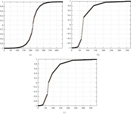
Figure_{7: The abscissa valuesxn}

mobtained with the sampling schemesα(a),β(b), andγ(c).

The presented design was implemented using the soft-wares Integrated Software Environment (ISE) and System Generator (SysGen) from Xilinx, on a Spartan-3 develop-ment kit from Avnet with a XC3S2000-5 FG676 Spartan 3 FPGA. The synthesis details of this realization can be seen on

Table 3.

4. Programmable Noise Generator

As a study case, the proposed nonuniform LUT-based inter-polator was used as a programmable noise generator able to output noise with different Probability Density Functions (PDFs). A controlled level of approximation error is achieved by using the proposed programmable nonuniform sampling scheme.

A given transformation functiong(x) is responsible for changing the PDF of a source uniformly distributed noise into a noise with a different and configurable PDF. The configuration parameters presented as an example in Tables

1and2were constructed having in mind the minimization of the approximation error of a Gaussian noise generator.

It uses a specificg1(x) transformation function [20],

repre-sented in (14), for transforming a uniform distributed noise into a Gaussian one:

g1(x)=

√

2σyerf−1(x). (14)

The transformation functiong1(x) has two poles located

at the abscissas x _{= −}1 and x ₌ +1, which are characterized by high values of curvature and derivatives. Both the uniformly distributed input signal and the domain of g1(x) are represented by the interval [x1,xP+1) =

[−1, +0.99993896484375). The ordinate of this function ideally goes from −∞ to +∞, what is expected since the output is an unlimited normally distributed signal.

One advantage of implementing a nonuniform sampling scheme for the interpolation of g1(x) is the lower RAM

space necessary for storing both theg1(xnm) ordinates and

g′

1(xnm) derivatives, allied to a lower approximation error.

−3

−2

−1 0 1 2 3

−1 −0.8 −0.6−0.4 −0.2 0 0.2 0.4 0.6 0.8 1 ×10−5

(a)

−1 −0.8 −0.6 −0.4 −0.2 0 0.2 0.4 0.6 0.8 1 ×10−3

−1

−0.8

−0.6 −0.4

−0.2 0 0.2 0.4 0.6 0.8 1

(b)

×10−3

−1 −0.8 −0.6 −0.4 −0.2 0 0.2 0.4 0.6 0.8 1 −1

−0.5 0 0.5 1

(c)

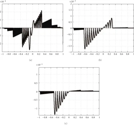
Figure_{8: Approximation error obtained for the Displaced Error Function (15) using the sampling schemesα(a),β(b), andγ(c).}

graphs show the absolute approximation error verified when two di_fferent uniform sampling schemes were applied to the whole [x1,xP+1) domain: the upper graph shows the error for fn = 128, what requires the storage ofin = 256 positions of g1(xnm) ordinates plus in = 256 for g1′(xnm) derivatives;

and the lower graph (observe the zoom on x axis) shows the error for the case where fn = 16384, that results in

in = 32768 + 32768 = 65536 positions for both RAM blocks. The horizontal line inFigure 3represents a boundary approximation error limit equal to 3.0518×10−5_{: the input}

values are 15 bits long, and any error lower than that boundary does not decrease the quality of the interpolation. If a uniform sampling scheme is used, the only solution to keep the absolute approximation error below this bound-ary for all abscissas x would be to use fn = 32768, what makes the approximation error equal to zero for all possible abscissasx. This happens because, in this extreme case, there

is not a really interpolation, but a one-to-one mapping of all possible input valuesx. But such linear sampling scheme requires a RAM block with a high depth equal toin=65536 positions for storingg1(xnm), hard to implement on an FPGA

due to the number of bits necessary to represent each stored value.

The solution is to use the proposed nonuniform sam-pling scheme which stores lessg1(xnm) ordinates andg1′(xnm)

derivatives for input values aroundx=0, and more samples near the polesx=+1 andx= −1, where the approximation error is bigger, saving significant amount of memory space (the proposed LUT-based interpolator reserves only 512 positions for each ordinate and derivative RAM blocks). This approach is graphically presented in Figure 4, where you can see the 1st quadrant ofg1(x)—the 3rd quadrant is

−2 −1 0 1 2

×10−4

−1 −0.8 −0.6 −0.4 −0.2 0 0.2 0.4 0.6 0.8 1

(a)

−2 −1.5

−1

−0.5 0 0.5 1 1.5 2

×10−3

−1 −0.8 −0.6 −0.4 −0.2 0 0.2 0.4 0.6 0.8 1

(b)

−0.5

−1 0 0.5 1

×10−3

−1 −0.8 −0.6 −0.4 −0.2 0 0.2 0.4 0.6 0.8 1

(c)

Figure_{9: Approximation error obtained for the Cubic Function (18) using the sampling schemesα(a),β(b), andγ(c).}

nonuniform approach remains under the boundary limit (3.0518×10−5_{) even near the poles of g}

1(x), as seen in

Figure 5.

When the proposed programmable nonuniform LUT-based interpolator is configured to represent (14), according to the sampling scheme of Tables 1 and 2, it works as a Gaussian noise generator: by applying to its input a signal with a uniform PDF (Figure 6(a)), it outputs a signal with Gaussian PDF (Figure 6(b)).

Tables1and2are just one example of configuration data for the proposed programmable LUT-based interpolator. In this work, 3 different sampling schemes (α, β, and γ) were formulated. The sampling scheme α was the one demonstrated in Tables 1 and 2. The abscissas xnm of

sampling schemesα,β, andγare plotted inFigure 7. As can be seen in these figures, there are P

n=1in = 445 sampling points on scheme α, P

n=1in = 374 on scheme β, and P

n=1in = 390 on scheme γ. As expected, the amount of sampling points is always smaller than the depth (equal to

512) of the two RAM blocks that store the corresponding ordinates g(xnm) and derivatives g′(xnm). Observe that the

inclination on these graphs is inversely proportional to the sampling frequency fn of each partition n: the higher the frequency fn, the bigger the number of abscissasxnm, and the

smaller the inclination inFigure 7.

To show the flexibility of the proposed design, the three sampling schemes (α,β, andγ) discussed above were applied to eight di_fferentg(x) transformation functions, represented by (14) to (21), which gave us a total of 24 di_fferent examples for configuring the proposed LUT-based interpolator. These equations were selected as mathematical examples, and they are not related to the generation of noise with a natural response:

g2(x)=3 +

√

2σyerf−1(x), (15)

g3(x)= − 1

0 1 2 3 4 5 6

×104

0 0.5 1 1.5 2 2.5 3 3.5 4 4.5

(a)

0 1 2 3 4 5 6 7 8 9 10

×104

−1 −0.8 −0.6 −0.4 −0.2 0 0.2 0.4 0.6 0.8 1

(b)

×104

0 1 2 3 4 5 6 7 8

0 0.1 0.2 0.3 0.4 0.5 0.6 0.7 0.8 0.9 1

(c)

×104

0 1 2 3 4 5 6 7

−1 −0.5 0 0.5 1 1.5 2 2.5 3

(d)

Figure_{10: Probability density function (PDF) of the output signal obtained with the sampling schemeαand the following functions ((a) to} (d)): Displaced Error Function (15), Cubic Function (18), first (19) and second Quadratic Function (20).

g4(x)=ex, (17)

g5(x)=x3, (18)

g6(x)=x2, (19)

g7(x)= −x2−2x−2, (20)

g8(x)=x2−6x−25. (21)

Each sampling scheme was designed to minimize the approximation error for xabscissa values belonging to the sampling region with higher fn values. As a matter of fact, high frequencies should be used for regions where g(x) presents a strong nonlinear behavior and low frequencies for regions with a linear behavior. For example, the sam-pling scheme α was specifically designed for the Gaussian transformation function (14). It applies high frequencies (fn = 16384) near the poles x = +1 and x = −1 and

low frequencies (fn = 32) near the origin x = 0. The approximation error for the three sampling schemesα,β, and

γ can be seen in Figure 8, in a case of using the displaced Gaussian transformation function (15), and inFigure 9, for the Cubic Function (18) case.

The frequency assignment of the P = 22 partitions for sampling schemesβ andγ is presented inTable 4. The corresponding configuration parameters for these sampling schemes are calculated via (2) to (12) and are presented in Tables 5 and 6. Observe that the sampling limits xn for sampling scheme β are the same as sampling scheme

α, only the frequencies fn are distributed differently. But in the sampling scheme γ, both sampling limits xn and the frequencies fnare distributed differently from sampling schemesαandβ, what shows the flexibility for reconfiguring the designed programmable noise generator.

lower frequencies near the origin, as can be graphically seen in Figures8and9(upper graphs): the semiarcs with bigger diameters (related to fn=32) are located around the origin, in the interval−0.125 < x < 0.125. As seen inTable 4, the schemesβandγ distribute the lower sampling frequencies (fn=32) on the intervals−0.64< x <0.34 and−0.5< x < 0.0, respectively, as can be graphically seen in Figures8and

9((b) and (c) graphs, resp.).

The designed programmable noise generator can gen-erate different noise signals by properly filling the ordinate

g(xnm) and the derivativeg′(xnm) RAM blocks (Figure 1) and

configuring its internal parameters on theDifference Address subsystem (Figure 2). For example, Figure 10 shows the Probability Density Functions (PDFs) of four di_fferent signals produced by the programmable noise generator when: (1) its input is fed with a uniform distributed noise, (2) it is configured with the sampling schemeα, and (3) it was configured to interpolate four different functions: the Displaced Error Function (15), the Cubic Function (18), the first (19), and the second (20) Quadratic Function.

5. Conclusion

A programmable Look-Up Table-based interpolator with nonuniform sampling scheme was implemented using a Avnet development kit containing an XC3S2000-5 FG676 Xilinx Spartan-3 FPGA. This LUT-based interpolator can be programmed on the fly by loading the proper configuration parameters presented in Section 2, including the g(xnm)

ordinate and g′_(x

nm) derivative, inside RAM blocks. The

complete reconfiguration takes 512 clocks cycles. When these parameters are changed, they can interpolate different

g(x) functions, sampled according to different nonuniform sampling schemes. The ability of changing the sampling scheme allows the minimization of both the approximation error and memory space: for instance, the sampling schemaα

(Table 1) applied to (14) was able to keep the approximation error below a threshold of 3.0518_×10−5 _{while reducing}

the memory usage to 2.71% for a Gaussian noise generator application.

As a study case, the LUT-based interpolator was used as the core of a programmable noise generator able to output signals with different Probability Density Functions (PDFs). The flexibility of this design was proved by interpolating 8 differentg(x) functions, according to 3 different nonuniform sampling schemes (α,β, andγ) described in Tables1and4, each one definingP=22 partitions each characterized by a chosen sampling frequency fn.

As future work, we recommend the implementation of a programmable nonuniform LUT-based interpolator with a domain not fixed to [x1,xP+1)= [−1, +1) and where the

numberPof sampling regions can be changed on the fly.

References

[1] K. Stewart, “Non-technical interoperability: the challenge of command leadership in multinational operations,” Tech. Rep., DTIC Document, 2004.

[2] P. Reddy, “Joint interoperability: Fog or lens for joint vision 2010,” Tech. Rep., DTIC Document, 1997.

[3] A. Tolk, Beyond Technical Interoperability—Introducing A Reference Model for Measures of Merit for Coalition Interoper-ability, Edited by O. D. U. N. Va, Citeseer, 2003.

[4] P. Van Oorschot, A. Menezes, and S. Vanstone,Handbook of Applied Cryptography, Crc Press, 1996.

[5] M. McLoone and J. V. McCanny, “Rijndael FPGA imple-mentations utilising look-up tables,” Journal of VLSI Signal Processing, vol. 34, no. 3, pp. 261–275, 2003.

[6] U. Farooq, Z. Marrakchi, H. Mrabet, and H. Mehrez, “The effect of LUT and cluster size on a tree based FPGA architecture,” inProceedings of the International Conference on Reconfigurable Computing and FPGAs (ReConFig ’08), pp. 115– 120, December 2008.

[7] K. H. Lee, D. H. Youn, and C. Lee, “An area-efficient interpolation filter using block structure,” inProceedings of the 8th IEEE International Conference on Electronics, Circuits and Systems (ICECS ’01), vol. 2, pp. 925–928, September 2001. [8] S. N. Ba, K. Waheed, and G. T. Zhou, “Efficient spacing

scheme for a linearly interpolated lookup table predistorter,” inProceedings of the IEEE International Symposium on Circuits and Systems (ISCAS ’08), pp. 1512–1515, May 2008.

[9] S. N. Ba, K. Waheed, and G. T. Zhou, “Optimal spacing of a linearly interpolated complex-gain LUT predistorter,”IEEE Transactions on Vehicular Technology, vol. 59, no. 2, pp. 673– 681, 2010.

[10] V. Monga and R. Bala, “Algorithms for color look-up-table (LUT) design via joint optimization of node locations and output values,” inProceedings of the IEEE International Conference on Acoustics, Speech, and Signal Processing (ICASSP ’10), pp. 998–1001, March 2010.

[11] D. Seidner, “Efficient iplementation of 10Y lookup table in FPGA,” inProceedings of the IEEE International Symposium on Industrial Electronics (ISIE ’09), pp. 686–689, July 2009. [12] L. Colavito and D. Silage, “Composite look-up table Gaussian

pseudo-random number generator,” in Proceedings of the International Conference on ReConfigurable Computing and FPGAs (ReConFig ’09), pp. 314–319, December 2009. [13] S. Shah, R. Velegalati, J. P. Kaps, and D. Hwang, “Investigation

of DPA resistance of block RAMs in cryptographic implemen-tations on FPGAs,” inProceedings of the International Confer-ence on Reconfigurable Computing and FPGAs (ReConFig ’10), pp. 274–279, December 2010.

[14] M. Vazquez, G. Sutter, G. Bioul, and J. P. Deschamps, “Decimal adders/subtractors in FPGA: efficient 6-input LUT imple-mentations,” inProceedings of the International Conference on ReConFigurable Computing and FPGAs (ReConFig ’09), pp. 42–47, December 2009.

[15] Z. Yan and A. M¨ammel¨a, “Comparison of look-up table minimization methods for real-time power amplifier simula-tion,” inProceedings of the IEEE Workshop on Signal Processing Systems—Design and Implementation (SiPS ’05), pp. 629–634, November 2005.

[16] J. K. Cavers, “Optimum table spacing in predistorting ampli-fier linearizers,”IEEE Transactions on Vehicular Technology, vol. 48, no. 5, pp. 1699–1705, 1999.

[18] S. Boumaiza, J. Li, M. Jaidane-Saidane, and F. M. Ghannouchi, “Adaptive digital/RF predistortion using a nonuniform LUT indexing function with built-in dependence on the amplifier nonlinearity,” IEEE Transactions on Microwave Theory and Techniques, vol. 52, no. 12, pp. 2670–2677, 2004.

[19] E. Dutra, L. Indrusiak, and M. Glesner, “Non-linear address-ing scheme for a lookup-based transformation function in a reconfigurable noise generator,” inProceedings of the 18th Symposium on Integrated Circuits and Systems Design (SBCCI ’05), pp. 242–247, September 2005.