This is a repository copy of
Unsupervised detector adaptation by joint dataset feature
learning
.
White Rose Research Online URL for this paper:
http://eprints.whiterose.ac.uk/84866/
Version: Accepted Version
Proceedings Paper:
Htike, KK and Hogg, D (2014) Unsupervised detector adaptation by joint dataset feature
learning. In: Chmielewski, LJ, Kozera, R, Shin, B-S and Wojciechowski, K, (eds.)
Computer Vision and Graphics International Conference, ICCVG 2014, Proceedings.
International Conference, ICCVG, 15-17 Sep 2014, Warsaw. Springer Verlag , 270 - 277.
ISBN 978-3-319-11331-9
[email protected] https://eprints.whiterose.ac.uk/
Reuse
Unless indicated otherwise, fulltext items are protected by copyright with all rights reserved. The copyright exception in section 29 of the Copyright, Designs and Patents Act 1988 allows the making of a single copy solely for the purpose of non-commercial research or private study within the limits of fair dealing. The publisher or other rights-holder may allow further reproduction and re-use of this version - refer to the White Rose Research Online record for this item. Where records identify the publisher as the copyright holder, users can verify any specific terms of use on the publisher’s website.
Takedown
If you consider content in White Rose Research Online to be in breach of UK law, please notify us by
Joint Dataset Feature Learning
Kyaw Kyaw Htike and David Hogg
School of Computing, University of Leeds Leeds, UK
{sckkh, d.c.hogg}@leeds.ac.uk
Abstract. Object detection is an important step in automated scene
un-derstanding. Training state-of-the-art object detectors typically require manual annotation of training data which can be labor-intensive. In this paper, we propose a novel algorithm to automatically adapt a pedestrian detector trained on a generic image dataset to a video in an unsupervised way using joint dataset deep feature learning. Our approach does not re-quire any background subtraction or tracking in the video. Experiments on two challenging video datasets show that our algorithm is effective and outperforms the state-of-the-art approach.
1
Introduction
Object detection has received a lot of attention in the field of Computer Vision. Pedestrians are one of the most common object categories in natural scenes. Most state-of-the-art pedestrian detectors are trained in a supervised fashion using large publicly available generic datasets [1, 2].
However, it has been recently shown that every dataset has an inherent bias [11]. This implies that a pedestrian detector that has been specifically trained for (and is tuned to) a specific scene would do better than a generic detector for that scene. In fact, it has been shown that generic detectors often exhibit unsatisfactory performance when applied to scenes that differ from the original training data in some ways (such as image resolution, camera angle, illumination conditions and image compression effects) [2].
We tackle this problem by formulating a novelunsupervised domain adapta-tion framework that starts with a readily available generic image dataset and automatically adapt it to a target video (of a particular scene) without requiring any annotation in the target scene, thereby generating ascene-specificpedestrian detector.
Domain adaptation for object detectors is a relatively new area. Most state-of-the-art research use some variations of an iterative self-training algorithm [12, 7]. Unfortunately, self-training carries the risk of classifierdrifting. In this paper, we investigate a different approach: domain adaptation purely by exploiting the
manifold propertyof data.
2 K. Htike and D. Hogg
learnt using unsupervised approaches. The most relevant works to our research in this area are [6, 5]. Gopalanet al. [6] propose building intermediate represen-tations between source and target domains by using geodesic flows. However, their approach requires sampling a finite number of subspaces and tuning many parameters such as the number of intermediate representations.
Gong et al. [5] improved on [6] by giving a kernel version of [6]. However both [6, 5] are dealing with only image data for both source and target domains and not videos. For videos, unique challenges are present such as the largely imbalanced nature of positive and negative data. Moreover, their approach does
notlearn deep representations required for manifolds that are highly non-linear. In this paper we propose, using state-of-the-art deep learning, to learn the nonlinear manifold spanned by the union of the source image dataset and the sampled data of the target video. The intuition is that by learning a represen-tation in that manifold and training a classifier on data in that represenrepresen-tation, the resulting detector would generalize well for the target scene. This can then be used as a scene-specific detector.
Contributions. We make the following novel contributions:
1. An algorithm that adapts a pedestrian detector from an imagedataset to a
videousing only the manifold assumption.
2. An application of state-of-the-art deep feature learning for detector adapta-tion invideosand showing its effectiveness. Furthermore, instead of starting with raw pixel values (as in standard deep learning), our approach takes as input, features such as Histogram of Oriented Gradients (HOGs) [1]. 3. For videos, due to huge class imbalance, random sampling of data will result
in almost all samples to be from non-pedestrian class. We propose a simple and effective biased sampling approach to minimize this problem.
4. A technique to automatically set the deep network structure with no tuning. 5. The integration of all of the above components into a system.
2
Proposed Approach
2.1 Overview
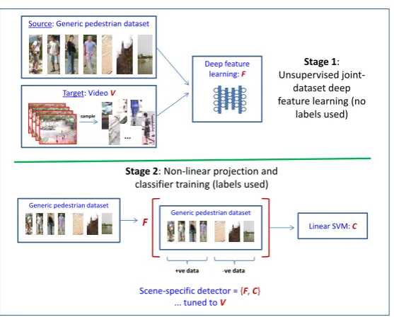
The overview of the algorithm is illustrated in Fig. 1. The algorithm is made up of two stages: (1) unsupervised deep feature learning (no supervision labels used) and (2) non-linear projection and classifier training (with labelled data). We use HOGs as the base features (before learning higher non-linear represen-tations). In Fig. 1, we have omitted the HOG feature extraction for clarity. Our algorithm can work with any type of base features and classifier combination. However, for simplicity, we use HOGs and a linear Support Vector Machine (SVM) respectively.
Let the generic pedestrian dataset G ={Gpos, Gneg} be a set of fixed-sized pedestrian and non-pedestrian patches, Gpos = {p+1, p
+ 2, . . . , p
+
N1} and Gneg = {p−
Source: Generic pedestrian dataset
Target: Video V
Deep feature learning:F
Linear SVM: C
Scene-specific detector = {F, C} ... tuned to V
Stage 1: Unsupervised
joint-dataset deep feature learning (no
labels used)
Stage 2: Non-linear projection and classifier training (labels used)
Generic pedestrian dataset
Generic pedestrian dataset
F
+ve data -ve data sample
[image:4.595.170.449.111.335.2]...
Fig. 1.Overview of the proposed algorithm.
N2 is the number of non-pedestrian patches. Let the target video be V =
{I1, I2, . . . , IM} where M is the number of frames in V. Furthermore, let the Hbe the function to extract base features on a given image patch.
Algorithm 1 describes the detector adaptation process. The patches obtained from the generic datasetGare combined with the patches sampled from the tar-get videoV. The sampling technique is detailed in Algorithm 2. After obtaining all the patchesDpatches, we extract HOG features from each of them, producing a feature vector for each patch. These feature vectors are input to the deep learn-ing algorithm described in Algorithm 3. The deep learnlearn-ing algorithm produces,
as output, a function H which takes in a HOG feature vector and produces a
feature vector of much smaller dimension by projecting the HOG feature vector onto the learnt manifold. We then project all the HOG features of the positive and negative data of the generic dataset into this space and train a linear SVM.
Algorithm 1Detector adaptation overview
Input: G,V,H
Output: Scene-specific detector ={F,C}
1: Dpatches← G
2: S←SamplePatchesFromVideo(V,G,H)
3: Dpatches←Dpatches∪S
4: D← H(Dpatches)
5: F= LearnDeepFeatures(D)
6: C= TrainSVM(F(H(Gpos)),F(H(Gneg)))
4 K. Htike and D. Hogg
Algorithm 2Biased sampling of patches from video
Input: V,G,H
Output: Sampled patches,Dpatches
1: C= TrainSVM(H(Gpos),H(Gneg))
2: SampleN frames fromV.
3: Run sliding-window detector withC on theN sampled frames
4: Dpatches←positive detections from detector
5: return Dpatches
Algorithm 3Deep Feature Learning
Input: HOG features,D
Output: Learnt non-linear projection function,F
1: Apply PCA onDand keep 99% variance 2: D←ProjectDonto principal component space 3: ndimsIn←number of dimensions ofD
4: Estimate intrinsic dimension ofDusing [8] 5: ndimsOut←Estimated intrinsic dimension 6: A ←SetUpAutoEncoder(ndimsIn,ndimsOut) 7: A ←initialiseAusing [4]
8: A ←Min LossFunc(A,D) using mini-batch L-BFGS 9: F ←Remove the decoder part ofA
10: return F
2.2 Sampling representative data from video
Although we are not concerned with any supervision labels during the fea-ture learning stage, we would like to get a mixfea-ture of both pedestrian and non-pedestrian patches from the video. However, naive random sampling of pedestrian-sized patches from video in the space of multi-scale sliding windows would result in pedestrian patches being sampled only with extremely low proba-bility. Therefore, we propose a biased sampling strategy as given in Algorithm 2.
2.3 Deep feature learning
In order to learn deep non-linear features, we use a deep autoencoder. We do not use any layer-wise stacked pre-training for initialization since recent research [10, 9] has shown that one of the main problems with deep networks ispathological curvaturewhich looks like local optima to 1st-order optimization techniques such as gradient descent, but not to 2nd-order optimization methods.
Data normalization & intrinsic dimensionality estimation. We first perform PCA and keep 99% of the total variance to condition the data for faster convergence during subsequent deep learning. After projecting the data using PCA coefficients, we estimate the intrinsic dimensionality of the data using [8].
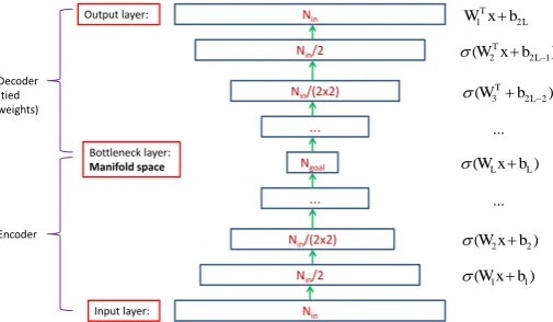
Setting up the deep autoencoder architecture & initialization. The ar-chitecture is shown in Fig. 2. Note that the network structure is obtained auto-matically and systeauto-matically and we do not have to manually tune it. After the network has been set up, we randomly initialize it using the method in [4].
Nin Nin/2
Nin/(2x2) ... Ngoal
... Nin/(2x2)
Nin/2
Nin Bottleneck layer: Manifold space Input layer: Output layer: Decoder (tied weights) Encoder ) (W1xb1
) (W2xb2
) (WLxbL
) ( 3 2L2
T
b W
) ( 2 2L1
T b x W L T b x W1 2
[image:6.595.181.434.252.399.2]... ...
Fig. 2.The deep autoencoder architecture.Nin is the number of data dimensions
af-ter normalization.Ngoalis the automatically estimated intrinsic dimensionality. Each
hidden layer has half of the number of hidden neurons as its previous layer and this is repeated until Ngoal is reached. After that, the decoding layers is mirrored to the
encoding layers. The encoding and decoding parts are symmetric and weights are tied (but not the biases). All hidden layers have hyperbolic tangent nonlinearity activation (represented by σ(•)). There are a total ofL hidden nonlinear layers in the encoder (which produces a total of 2Llayers feed-forward neural network.)
Network optimization. In order to train the autoencoder, the network in Fig. 2 can be mathematically written as a smooth differentiable multivariate loss function which should be minimized. This is given in Equation 1; mrefers to the number of data in each mini-batch,Wj is affine projection matrix for layer
j,x(i) is a column vector of data pointiandb
j is a vector of bias for layerj.
arg min
W1,...,WL,
b1,...,b2L
1 2m m X i=1 L X j=1
σ(Wjx(i)+bj) +
2L−1 X
j=L+1
σ(W(2TL−j+1)x (i)+
bj)+
WT
6 K. Htike and D. Hogg
Removing the decoding part. After training the deep network, the decoder part is no longer needed and is thus removed. We now have a deep non-linear projection functionF with the number of projection layers given byL.
2.4 Training scene-specific detector
We use the learnt encoder,F, to project the generic datasetGand train a SVM on these features. This is illustrated in Fig. 3.
Nin
Nin/2
Nin/(2x2)
... Ngoal
Bottleneck layer: Manifold space
Input layer: Encoder
) (W1xb1
) (W2xb2
) (WLxbL
...
Linear SVM
pos
[image:7.595.176.440.229.354.2]G Gneg
Fig. 3.Training the scene-specific detector.
3
Experimental Results
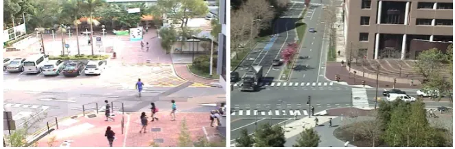
Datasets. INRIA pedestrian dataset [1] is used as the source dataset. We eval-uate on two target datasets: CUHK Square (a 60 mins video) and MIT Traffic (90 mins) [12]. Frame samples are shown in Fig. 4. Each dataset is divided into two halves: the 1sthalf is used for unsupervised detector adaptation and the 2nd half for quantitative evaluation. These datasets are very challenging: they vary greatly from the INRIA dataset in terms of resolution, camera angle and poses.
[image:7.595.141.473.518.627.2]Deep learning parameters. For CUHK experiments, the layer sizes for en-coder part of the deep network are found to beE = [1498,749,375,187,94,35]. The decoder layer sizes are D = [94,187,375,749,1498]. The complete layer sizes for the whole network is therefore given by R = [E,D]. The first and last elements ofRcorrespond to input and output layer sizes respectively (i.e. the number of dimensions after PCA projection) and the ones in the middle are hidden layers. In this case, 35 is the size of the bottleneck layer. For MIT,
E = [1536,768,384,192,96,48,23]. Mini-batch size for training is fixed at 1000 for both CUHK and MIT.
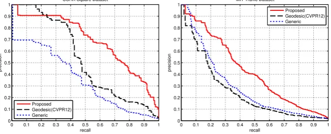
Evaluation and discussion. We use precision-recall (PR) curves in order to compare the performance. Detection bounding boxes are scored according to the PASCAL 50% overlap criteria [3]. Average Precision (AP) is calculated for each PR curve by integrating the area under the curve. For each target dataset, we perform 3 different types of experiments:
1. Generic: The detector (HOG+SVM) trained on INRIA dataset. This is the baselinewithoutany domain adaptation.
2. Geodesic(CVPR12): The approach proposed by Gonget al. [5]. We use the code made available by them and extend it to be applicable to video. 3. Proposed: Our proposed detector adaptation algorithm.
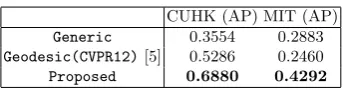
The PR curves are shown in Fig. 5 and the corresponding APs are shown in Table 1. As can be seen, our algorithm (Proposed) outperforms the base-line (Generic) and the state-of-art (Geodesic) in both datasets. For CUHK,
Proposedachieves almost twice the AP of baseline (0.6880 vs. 0.3554), whereas
Geodesic has less improvement over the baseline (0.5286 vs. 0.3554).
Interest-ingly, for MIT, Geodesicperforms worse than the baseline whereas Proposed
clearly improves over the baseline and attains an AP which is around 1.5 times that of the baseline. This suggests that for the MIT traffic dataset, which is a more difficult dataset than the CUHK dataset (partly due to much lower reso-lution), the state-of-the-artGeodesicfails to improve over the baseline whereas
0 0.1 0.2 0.3 0.4 0.5 0.6 0.7 0.8 0.9 1 0
0.1 0.2 0.3 0.4 0.5 0.6 0.7 0.8 0.9 1
recall
precision
CUHK Square Dataset
Proposed Geodesic(CVPR12) Generic
0 0.1 0.2 0.3 0.4 0.5 0.6 0.7 0.8 0.9 1 0
0.1 0.2 0.3 0.4 0.5 0.6 0.7 0.8 0.9 1
recall
precision
MIT Traffic Dataset
[image:8.595.141.478.517.653.2]Proposed Geodesic(CVPR12) Generic
8 K. Htike and D. Hogg
[image:9.595.222.394.163.208.2]our approach, due to unsupervised learning of deep non-linear features and the resulting implicit manifold regularization, achieves much better results.
Table 1.Average precision results
CUHK (AP) MIT (AP)
Generic 0.3554 0.2883
Geodesic(CVPR12)[5] 0.5286 0.2460
Proposed 0.6880 0.4292
4
Conclusion
In this paper, we propose an algorithm to automatically generate a scene-specific pedestrian detector that is tuned to a particular scene by unsupervised domain adaptation of a generic detector. Our algorithm learns the underlying manifold where both the generic and the target dataset jointly reside and a detector is trained in this space, implicitly regularized to perform well on the target scene. Evaluation on two public video datasets show the effectiveness of our approach.
References
1. Dalal, N., Triggs, B.: Histograms of oriented gradients for human detection. In: CVPR (1). pp. 886–893 (2005)
2. Doll´ar, P., Wojek, C., Schiele, B., Perona, P.: Pedestrian detection: A benchmark. In: CVPR. pp. 304–311 (2009)
3. Everingham, M., Gool, L.J.V., Williams, C.K.I., Winn, J.M., Zisserman, A.: The pascal visual object classes (voc) challenge. International Journal of Computer Vision 88(2), 303–338 (2010)
4. Glorot, X., Bengio, Y.: Understanding the difficulty of training deep feedforward neural networks. In: International Conference on Artificial Intelligence and Statis-tics. pp. 249–256 (2010)
5. Gong, B., Shi, Y., Sha, F., Grauman, K.: Geodesic flow kernel for unsupervised domain adaptation. In: CVPR. pp. 2066–2073 (2012)
6. Gopalan, R., Li, R., Chellappa, R.: Domain adaptation for object recognition: An unsupervised approach. In: ICCV. pp. 999–1006 (2011)
7. Kevin Tang, Vignesh Ramanathan, L.F.F.D.K.: Shifting weights: Adapting object detectors from image to video. In: Neural Information Processing Systems (NIPS) (2012)
8. Levina, E., Bickel, P.J.: Maximum likelihood estimation of intrinsic dimension. In: Advances in neural information processing systems. pp. 777–784 (2004)
9. Martens, J.: Deep learning via hessian-free optimization. In: Proceedings of the 27th International Conference on Machine Learning (ICML-10). pp. 735–742 (2010) 10. Ngiam, J., Coates, A., Lahiri, A., Prochnow, B., Ng, A., Le, Q.V.: On optimization methods for deep learning. In: Proceedings of the 28th International Conference on Machine Learning (ICML-11). pp. 265–272 (2011)
11. Torralba, A., Efros, A.A.: Unbiased look at dataset bias. In: Computer Vision and Pattern Recognition (CVPR), 2011 IEEE Conference pp. 1521–1528. IEEE (2011) 12. Wang, M., Li, W., Wang, X.: Transferring a generic pedestrian detector towards