sampling platforms to assess deep-water
rocky reef ecosystems on the
continental shelf
Jan Seiler
BSc (Applied Marine Biology)
Submitted in fulfilment of the requirements for the Degree of Doctor
of Philosophy, in the CSIRO-UTAS PhD Program in Quantitative
Marine Science
at University of Tasmania.
I declare that this thesis contains no material which has been
accepted for a degree or diploma by the University or any other
institution, except by way of background information and duly
acknowledged in the thesis, and to the best of my knowledge
and belief no material previously published or written by another
person except where due acknowledgement is made in the text of
the thesis, nor does the thesis contain any material that infringes
copyright.
The publishers of the papers comprising Chapters 3 and 5 hold the
copyright for that content, and access to the material should be
sought from the respective journals. The remaining non published
content of the thesis may be made available for loan and limited
copying and communication in accordance with the Copyright Act
1968.
Jan Seiler
Traditional extractive sampling methods, such as netting and trawling, to assess
benthic species diversity, size and abundance are unable to sample complex hard
substrates, e.g., rocky reefs. This inability led to the development of alternative
non-extractive sampling platforms, such as digital stills and video cameras mounted
onto stationary or moving platforms. This thesis examined two moving platforms,
autonomous underwater vehicle (AUV) and towed video platform and one stationary
platform, stereo baited underwater video systems (BUVS). These platforms were
used as sampling tools to assess reef fish diversity, size distribution and absolute
and relative abundance in complex deep-water (30 – 100 m) rocky reefs in temperate
Australia (Tasmania). Each platform was evaluated with respect to their efficiency
and reliability within a sustainable resource management framework. A novel feature
extraction routine, using colour, texture, patch-gap summaries and rugosity, to
semi-automatically classify AUV images into habitat classes is proposed. Here,
the randomForest classification tree algorithm was used to assign habitat classes
to images after initial training (i.e., 500 images annotated by a trained human
expert). Classifier accuracy was assessed using this human scored image set. Habitat
prediction accuracy was 84% (with a kappa statistic of 0.793).
The evaluation of stereo BUVS as a tool to inventory and monitor deep-water
temperate reef fish diversity can inform resource managers of advantages and
abundance across different survey sites over two years were investigated. In addition,
stereophotogrammetric fish length estimation of two commercially important
species, striped trumpeter (Latris lineata) and blue-throated wrasse (Notolabrus
tetricus), were utilised to set a benchmark for future reference and compared to
line-fishing (L. lineata) and trapping data (N. tetricus).
All three platforms were compared to evaluate their ability to assess reef fish diversity
and abundance. Sample variability for each tool was assessed statistically and
synergy between platforms proposed. The cost-effectiveness of each platform was
assessed qualitatively.
An assessment of the size and abundance distribution of the ocean perch
Helicolenus percoides was conducted using photographic records taken by the AUV.
Stereophotogrammetric size estimates were converted into biomass and examined
with respect to depth and habitat types. Habitat preferences of adult and juvenile
ocean perch were also investigated. The results suggest that AUVSiriusis a mature
survey platform in complex hard substratum environments. The utility of this
non-extractive sampling tool in a fisheries context is discussed.
Non-extractive imagery-yielding sampling platforms provide useful alternatives
when sampling complex environments. Data quality, derived from imagery, is
benefitting from rapidly developing technology, e.g., high-definition video and
megapixel digital cameras. Non-extractive methods provide the only means to
sample marine protected areas. Advantages and disadvantages of each platform
are now readily accessible to advise resource management agencies.
Statement of Declaration i
Abstract iii
Contents vii
List of Figures xv
List of Tables xvii
Statement of co-author contributions xix
Acknowledgements xxiii
1 Introduction 1
1.1 In a nutshell . . . 1
1.2 Sustainable resource management – a fisheries example . . . 1
1.3 Australia’s recent EBM history . . . 3
1.4 Consequences of adopting EBM . . . 4
1.5 Current EBM challenges . . . 5
1.6 Solutions – thesis objectives . . . 7
1.7 Thesis outcomes and future research . . . 12
2.1 Introduction . . . 17
2.2 Study area . . . 18
2.3 Bathymetric mapping . . . 20
2.4 Autonomous Underwater Vehicle . . . 20
2.4.1 AUV camera calibration . . . 21
2.4.2 AUV sampling design . . . 23
2.4.3 AUV image annotation . . . 24
2.5 Baited Underwater Video Systems . . . 25
2.5.1 BUVS design and components . . . 26
2.5.2 BUVS camera calibration . . . 28
2.5.3 BUVS sampling design . . . 29
2.5.4 BUVS video annotation . . . 32
2.6 Towed video platform . . . 34
2.6.1 Towed video sampling design . . . 34
2.6.2 Towed video annotation . . . 36
3 Image-based continental shelf habitat mapping using novel automated data extraction techniques 39 3.1 Abstract . . . 39
3.2 Introduction . . . 40
3.3.1 Study area . . . 44
3.3.2 Data acquisition . . . 45
3.3.3 Automated feature extraction . . . 46
3.3.4 Modified hue-saturation values (HSV) . . . 47
3.3.5 Local binary pattern (LBP) . . . 49
3.3.6 Patch-gap summaries . . . 50
3.3.7 Deriving rugosity . . . 52
3.3.8 Manual image scoring . . . 52
3.3.9 Random forests classifier training and evaluation . . . 53
3.4 Results . . . 58
3.4.1 Prediction accuracy . . . 58
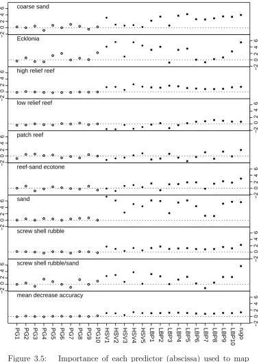
3.4.2 Predictor importance . . . 59
3.4.3 Confusion matrices . . . 60
3.4.4 χ2 and permutation . . . 62
3.4.5 Multi-dimensional scaling and proximity . . . 65
3.4.6 Habitat mapping . . . 66
3.5 Discussion . . . 69
assemblages on the continental shelf 75
4.1 Abstract . . . 75
4.2 Introduction . . . 76
4.2.1 Individual species abundances of reef fish assemblages . . . 80
4.2.2 Size structure of two commercial species . . . 81
4.2.3 Improving estimates of relative abundance . . . 82
4.2.4 Power analysis . . . 82
4.3 Material and Methods . . . 84
4.3.1 Composition of reef fish assemblages . . . 86
4.3.2 Individual species abundances of reef fish assemblages . . . 89
4.3.3 Size structure of two commercial species . . . 90
4.3.4 Improving estimates of relative abundance . . . 91
4.3.5 Power analysis . . . 93
4.4 Results . . . 95
4.4.1 Composition of reef fish assemblages . . . 95
4.4.2 Individual species abundances of reef fish assemblages . . . 99
4.4.3 Size structure of two commercial species obtained by photogrammetric length estimation . . . 101
4.4.4 Improving estimates of relative abundance . . . 108
4.5 Discussion . . . 114
4.5.1 Composition of reef fish assemblages . . . 114
4.5.2 Individual species abundances of reef fish assemblages . . . 117
4.5.3 Size structure of two commercial species obtained by photogrammetric length estimation . . . 118
4.5.4 Improving estimates of relative abundance . . . 121
4.5.5 Power analysis . . . 125
4.6 Conclusion . . . 126
5 Assessing size, abundance and habitat preferences of the ocean perch Helicolenus percoides using a AUV-borne stereo camera system 127 5.1 Abstract . . . 127
5.2 Introduction . . . 128
5.3 Material and Methods . . . 131
5.3.1 Field Sampling . . . 131
5.3.2 Data acquisition and processing . . . 133
5.3.3 Statistical analysis . . . 137
5.4 Results . . . 142
5.4.1 Measurement precision . . . 142
5.4.2 Habitat association and spatial autocorrelation . . . 142
5.4.3 Fish occurrence, length and biomass . . . 143
5.4.4 Habitat preferences . . . 148
5.5 Discussion . . . 151
5.5.1 Distribution and size composition of H. percoides across habitat types . . . 151
5.5.2 Improving efficiency and quality of image-based data . . . 154
5.5.3 Utility of AUV Siriusfor fishery assessments . . . 157
– a comparison 161
6.1 Abstract . . . 161
6.2 Introduction . . . 162
6.3 Materials and methods . . . 165
6.3.1 Study area and sites . . . 165
6.3.2 Sampling platforms . . . 166
6.3.3 Data analysis . . . 170
6.4 Results . . . 172
6.4.1 Species richness and total number of individuals . . . 172
6.4.2 Individual species abundances . . . 178
6.5 Discussion . . . 186
6.5.1 Platform strengths and weaknesses . . . 187
6.5.2 To bait, or not to bait . . . 192
6.5.3 Dissecting assemblage composition – platform-specific species detection . . . 195
6.5.4 Future research . . . 195
6.5.5 Concluding remarks . . . 196
7 Discussion and conclusion 197 7.1 Summary of achievements . . . 197
7.1.2 Mapping marine habitats – essential information for
sustainable resource management . . . 198
7.1.3 Beyond diver’s depth – assessing reef-fish assemblages using baited underwater video systems . . . 200
7.1.4 Collecting fisheries-independent stock assessment data using a stereo-vision AUV . . . 201
7.1.5 Observing deep-water temperate rocky reef fish assemblages on the continental shelf using three non-extractive sampling platforms . . . 202
7.1.6 Utilising non-extractive imagery-yielding samplers in an ecosystem-based management context . . . 203
7.2 Future research . . . 205
7.2.1 AUV . . . 205
7.2.2 BUVS . . . 208
7.2.3 Size selectivity . . . 210
7.3 Summary . . . 211
References 213
1.1 Schema diagram elucidating thesis structure . . . 15
2.1 Study area location . . . 19
2.2 Autonomous Underwater Vehicle schematic . . . 23
2.3 Schematic of BUVS unit . . . 28
2.4 Calibration cube . . . 30
2.5 Schematic of towed video system . . . 35
3.1 Study area off O’Hara Bluff with superimposed AUV transect . . . . 45
3.2 Schematic illustrating the concept of Local Binary Patterns (LBP) . . 50
3.3 Example images for each habitat class . . . 55
3.4 Comparison of different predictors . . . 59
3.5 Predictor importance . . . 61
3.6 Frequency of occurrence of observed and predicted habitat classes . . 64
3.7 Multi-dimensional scaling plot of the proximity matrix . . . 67
3.8 Colour-coded observed and predicted habitat classes . . . 68
4.1 Map depciting BUVS deployments . . . 85
4.2 Two-dimensional nMDS plot of inshore and offshore fish assemblages 97
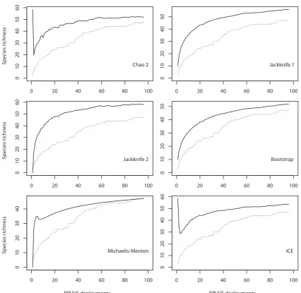
4.4 Species accumulation curve against estimates . . . 100
4.5 Size and weight frequency histogram of striped trumpeter . . . 104
4.6 Size frequency histogram of blue-throated wrasse . . . 106
4.7 N. tetricusby depth probability . . . 107
4.8 Barplot of fit and line plot of statistical power . . . 112
4.9 Line plot of statistical power and sample size . . . 113
5.1 AUV dive locations . . . 132
5.2 Calibration chequerboard . . . 135
5.3 PhotoMeasure user interface . . . 137
5.4 Histogram of measurement error . . . 143
5.5 Correlograms with 95% point-wise bootstrap confidence intervals . . . 144
5.6 Mean biomass in gram of H. percoides by habitat . . . 145
5.7 GLMM predicted probabilities ofH. percoides presence per image . . 147
5.8 Histograms ofH. percoides length and weight . . . 148
5.9 Habitat preference index by habitat . . . 150
5.10 Percentage of juveniles and adult fish by habitat . . . 151
6.1 AUV, BUVS, towed video sampling locations . . . 167
6.2 Barplot of mean species richness and total number of individuals at each site for each platform . . . 179
6.3 Barplot of selected mean species abundance at each site for each platform . . . 181
6.4 nMDS plot based on fourth-root transformed species composition . . 183
6.5 nMDS plot based on species presence/absence . . . 184
6.6 Species accumulation curve for each platform . . . 186
2.1 List of AUV specifications and sensors . . . 22
2.2 Habitat types scored during AUV image annotation with brief
description . . . 25
3.1 Overview of extracted image features and brief description . . . 48
3.2 Habitat class code, habitat class, brief habitat description and
frequency of occurrence . . . 54
3.3 Confusion matrix for habitat classification prediction . . . 63
4.1 Habitat complexity measures derived from DEM with definition and
references . . . 88
4.2 Total species richness estimates . . . 99
4.3 Species and common names and total MaxN count of the five most
numerous fish species in the BUVS data set . . . 99
4.4 Negative binomial GLM results comparing fish abundance between
inshore and offshore sites . . . 102
4.5 MaxNand Ncomparison L. lineata . . . 109
4.6 MaxNand Ncomparison N. tetricus. . . 111
4.7 Distribution and parameters µ and k used in the power analysis for
the three species . . . 113
5.1 ANOVA results for H. percoides biomass in response to habitat . . . . 148
6.1 Species list . . . 174
6.3 Univariate ANOVA results for C. lepidoptera and P. psittaculus
ln(x+ 1) transformed abundance data in response to site and platform.181
6.4 GLMs parameter estimates for untransformed Helicolenus percoides
and Nemadactylus macropterus counts . . . 182
6.5 PERMANOVA results based on Bray-Curtis dissimilarity of
fourth-root transformed relative abundance and presence/absence data. The two factors P and S refer to platform and site, respectively. . . 183
Chapters 3 and 5 of this thesis have been accepted for publication in peer-reviewed
journals. Research design and implementation, data analysis, interpretation of
results and manuscript preparation were the sole responsibility of the research
candidate in consultation with supervisors and with input from specialist
contributors.
The following people and institutions contributed to the publication of work
under-taken as part of this thesis:
Jan Seiler (University of Tasmania)
Ariell Friedman and Daniel Steinberg (University of Sydney)
Dr Alan Williams (CSIRO)
Dr Neville Barrett and Dr Neil Holbrook (University of Tasmania)
Author details and their roles:
The candidate was the primary author for the publication “Image-based continental
shelf habitat mapping using novel automated data extraction techniques”
Ariell Friedman and Daniel Steinberg extracted additional image features to extent
the suite of predictors for the random forests model. Dr Alan Williams, Dr Neville
Barrett and Dr Neil Holbrook provided advice on approaches to habitat mapping
and commented the manuscript.
Jan Seiler (University of Tasmania)
Dr Alan Williams (CSIRO)
Dr Neville Barrett (University of Tasmania)
Author details and their roles:
The candidate was the primary author for the publication “Assessing
size, abundance and habitat preferences of the Ocean perch Helicolenus
percoides using a AUV-borne stereo camera system” (Fisheries Research,
doi:10.1016/j.fishres.2012.06.011), located in chapter 5. Dr Alan Williams and Dr
Neville Barrett provided advice on approaches to assess benthic reef fish stocks and
commented the manuscript.
We the undersigned agree with the above stated “proportion of work undertaken” for
each of the above published (or submitted) peer-reviewed manuscripts contributing
to this thesis:
Neville Barrett
Supervisor Head of School
IMAS IMAS
University of Tasmania University of Tasmania
This work has been funded through the Commonwealth Environment Research
Facilities (CERF) program, an Australian Government initiative supporting world
class, public good research. The CERF Marine Biodiversity Hub is a collaborative
partnership between the University of Tasmania, CSIRO Wealth from Oceans
Flagship, Geoscience Australia, Australian Institute of Marine Science and Museum
Victoria. Logistic support for the AUV Sirius, used for this project, was provided
by the Australian Centre for Field Robotics at the University of Sydney and
the Integrated Marine Observing System (IMOS) - which collectively represents
nationally distributed equipment and data-information services. The assistance
and support of the following people is greatly appreciated; Colin Buxton and
Justin Hulls (Institute for Marine and Antarctic Studies, UTas), Stefan Williams,
Oscar Pizzaro, Michael Jakuba, Duncan Mercer and George Powell (University of
Sydney) and Matthew Francis and Jac Gibson (R/V Challenger crew). Richard
Coleman (Australian Research Council) initiated the use of the AUV in Tasmanian
waters. The gridded bathymetric dataset was collected and processed by Geoscience
Australia.
Chapter
1
Introduction
1.1
In a nutshell
Continental shelves provide more than 90% per cent of the world’s fisheries landings
and for 3 billion people, fish constitutes 15% of their animal protein intake
per capita (FAO, 2010). Rocky reefs are highly productive and an ecologically
important component of continental shelves due to their high species numbers and
habitat diversity (Taylor, 1998). Sustainable management of finite resources on the
continental shelf requires efficient and preferably non-extractive methods to assess
and monitor these assets. This thesis tests and evaluates three novel non-extractive
methods to sample marine resources with respect to efficiency and applicability to
current managerial needs such as habitat mapping and fisheries and conservation
management.
1.2
Sustainable resource management – a fisheries example
Traditional single-species fisheries management has often been ineffective as it
ignores ecosystem components of the target species such as habitat, predators
and prey (Pikitch et al., 2004). Over the past decade many nations adopted an
and the fisheries they support (Pikitch et al., 2004). This alternative is called
the Ecosytem-Based Fisheries Management (EBFM) or the ecosystem approach to
fisheries (Garcia et al., 2003). Ecosystem-based management (EBM) is not exclusive
to fisheries but finds application in contemporary ocean and living marine resource
management (Murawski, 2007). According to Pikitch et al. (2004) EBFM should
(i) avoid degradation of ecosystems, as measured by indicators of environmental
quality and system status; (ii) minimize the risk of irreversible change to natural
assemblages of species and ecosystem processes; (iii) obtain and maintain
long-term socioeconomic benefits without compromising the ecosystem; (iv) generate
knowledge of ecosystem processes sufficient to understand the likely consequences of
human actions. Where knowledge is insufficient, robust and precautionary fishery
management measures that favour the ecosystem should be adopted (Pikitch et al.,
2004). The central piece of legislation in Australia to address these four points
is the Environment Protection and Biodiversity Conservation Act 1999 (EPBC).
The EPBC Act provides a legal framework to protect and manage nationally and
internationally important flora, fauna and ecological communities (DSEWPC, 2012).
This includes measures to mitigate threats through global warming, i.e., sea-level rise
(to protect reef-forming corals) and increased occurrences of severe weather events
(cyclones and droughts) and reducing river pollution and sediment loads in rivers
(both are factors that affect mangrove forest and coral reef ecosystem health; Rogers
(1990); Fabricius et al. (2005)). Under the EPBC Act, the Australian Government
identified a network of marine reserves to halt the decline in biodiversity and
form part of this network with the following activities still allowed: recreational and
commercial fishing, marine tourism, charter boat operations (fishing), recreational
boating, mining and oil and gas activities and port development and shipping.
Protection of CMRs is provided by fishing gear restrictions, gear with no or
little impact on the benthic fauna, control over the extent of fishing activities,
environmental assessments before commencing mining and port development and
licensing for tourism and charter boat operators.
1.3
Australia’s recent EBM history
“Australia aims to realise its international commitments as a signatory to the
Convention on Biological Diversity through the significant expansion of its existing
MPA network throughout Australia’s Exclusive Economic Zone (EEZ) by 2012”
(DSEWPC, 2012). This expansion is achieved through the establishment of a
National Representative System of Marine Protected Areas (NRSMPA). “The
primary goal of the NRSMPA is to establish and manage a comprehensive, adequate
and representative system of marine protected areas to contribute to the long-term
ecological viability of marine and estuarine systems, to maintain ecological processes
and systems, and to protect Australia’s biological diversity at all levels” (DSEWPC,
2012). One of the secondary NRSMPA objectives is to provide scientific reference
sites. These reference sites provide a benchmark against which the effects of human
1.4
Consequences of adopting EBM
Currently, ∼ 880,000 km2 or 10% of Australia’s EEZ, excluding the Australian
Antarctic Territory are part of the NRSMPA (DSEWPC, 2012). However, only a
fraction of this area, usually areas in State coastal water and parts of the Great
Barrier Reef, has been inventoried or was subjected to baseline MPA monitoring
to capture the variability of natural processes. Actual knowledge of what the
NRSMPA comprise is so poorly known, that surveys of the Australian continental
shelf and slope typically find that 30 – 50% of the decapod species sampled are
new to science (Poore et al., 2008). Protected areas within the NRSMPA need to
contribute to the representativeness, comprehensiveness or adequacy of the national
system which, given the poor knowledge of what the areas actually comprise, is a
challenging prospect. This only highlights the difficulties encountered during the
planning phase regardless of meeting the 2012 target. Once established [NRSMPA],
the Environment Protection and Biodiversity Conservation Act requires an annual
environmental performance report. Currently, surveys of State managed marine
reserves provide the most comprehensive knowledge of continental shelf habitats and
therefore allow CAR (Comprehensive Adequate and Representative) principles to
be fully implemented. Consequently, adopting ecosystem-based management (EBM)
requires solutions to address (1) rapid resource and habitat mapping, (2) baseline
data to evaluate management strategies and (3) regular monitoring techniques.
With respect to habitat mapping in an EBM context, it is not sufficient to identify
above). Rather, EBFM should generate knowledge of ecosystem processes such as
fish-habitat associations and inter-habitat relationships.
1.5
Current EBM challenges
Qualitative and quantitative data are a prerequisite for managing coastal marine
resources. This knowledge is fundamental during the planning phase (inventory)
as well as after implementation (monitoring). Underwater visual census (UVC)
techniques are the most commonly used methods for monitoring biotic change in
coastal MPAs [Marine Protected Areas] (Barrett and Buxton, 2002). UVC is a
diver-based sampling method. Despite its [UVC] popularity it is ineffective in
sampling most managed fishing grounds and reserves; UVC is restricted to water
depths, that are safe for SCUBA divers (< 30 m). To address the critical need
for efficient sampling tools without depth restrictions, the Marine Biodiversity Hub
funded by the Commonwealth Environmental Research Facilities program tested and
integrated, relatively new survey technologies such as multibeam sonar, underwater
video and autonomous underwater vehicle (AUV) imagery (Bax, 2011; Brown et al.,
2011; Kostylev et al., 2001). Desirable characteristics of these new sampling
tools include being quantitative, non-extractive and suitable for monitoring, i.e.,
cost-effective and able to return to the exact sampling location for subsequent
surveys. Marine habitat maps are fundamental prerequisites for scientific fisheries
management and monitoring environmental changes and anthropogenic impacts on
benthic habitats (Kostylev et al., 2001; Diaz et al., 2004; Halpern et al., 2008;
bathymetrically mapped (Bax, 2011). This territory does not exceed 200 nautical
miles from the baseline, i.e., low water line along the coast, unless the geological
continental shelf extends beyond the 200 nm limit. Hence, the continental shelf
and slope, abyssal plains, canyons and other submarine features can occur within
this geologically arbitrary 200 nm limit. Current notable mapping coverage include
almost all MPAs in Australia, Cape Nelson, Victoria (Rattray et al., 2009) and the
Hopkins site in Victoria (Ierodiaconou et al., 2007). The aforementioned habitat
maps are based on multibeam sonar data (bathymetry and acoustic backscatter)
and fine-scale ground-truthing data using video imagery of the seafloor. Although
sonar data in isolation can provide coarse habitat maps using morphometric feature
classification (Lucieer and Pederson, 2008) they cannot provide ecologically more
meaningful maps of kelp forest, sponge garden or coral reef extent (Wilson et al.,
2007). Morphometric feature classification is based on nearest neighbour statistics
on gridded bathymetry data. For example, by examining relationships between
neighbouring grid cells and the central grid cell in a 3 × 3 window an algorithm
developed by Wood (1996) classifies each cell into one of six feature (habitat) classes:
plains, passes, ridges, peaks, channels or pits. However, the creation of ecologically
more meaningful habitat maps relies on the combination of bathymetric data and
fine-scale data obtained from grab samplers, sediment cores or imagery
(ground-truthing). In recent years multibeam sonar backscatter analysis has provided some
insight to the nature of seabed features such as hard or soft substratum (Hasan et al.,
2012). Both techniques in conjunction with ground-truthing, either extractive or
(Kostylev et al., 2001). Processing fine-scale (∼ 1 m2) samples is time-consuming
and resource-intensive. This processing stage is often considered the proverbial
bottleneck during map production. However, this extraction of information is
essential to acquire qualitative and quantitative data using fine-scale imagery.
1.6
Solutions – thesis objectives
As part of the Marine Biodiversity Hub this study tested and evaluated
imagery-yielding samplers that are non-extractive and quantitative. An advantageous
characteristic of imagery-yielding samplers is the permanent record and auxiliary
information contained in the imagery, e.g., the target species AND its environment.
Testing and evaluation was conducted under the following criteria: (1)
cost-effectiveness with respect to collecting an inventory of habitats and monitoring
fragile and/or protected environments, applicability to existing needs, e.g.,
fisheries-independent stock assessment, MPA planning and monitoring and habitat mapping.
Three different sampling tools were tested to address several challenges with respect
to the current EBM challenges outlined above.
Advanced habitat mapping techniques – chapter 3 (Seiler et al.,
doi.10.1016/j.csr.2012.06.003)
Almost 90% of Australia’s EEZ remains to be bathymetrically mapped. However,
within this 200 nm EEZ there are several geological features, such as the continental
continental shelf. Currently, multibeam echo sounders (MBES) are the only means
to efficiently fathom Australia’s continental shelves, especially areas with high
conservation value such as Australia’s MPAs. Most notable areas that were mapped
using scientific multibeam echo sounders are Jervis Bay, NSW (Anderson et al.,
2009) and the Freycinet and Huon Commonwealth Marine Reserves, TAS (Nichol
et al., 2009). However, the resolution and information provided by MBES alone
is insufficient at the habitat scale – the scale at which EBM [ecosystem-based
management] operates. At the habitat scale (area that comprises ecologically
linked multi-species assemblages, such as kelp, invertebrates and fish in a kelp
forest habitat), imagery-yielding samplers are the only means of mapping benthic
habitats on hard substrates such as sponge gardens or kelp forests on rocky reef
(Copeland et al., 2011). However, there are examples where Regional Marine
Planning is based on geomorphic features, such as continental rise, pinnacle, canyon,
terrace, trench/trough, etc, which are derived from grid-based terrain analysis
using multibeam bathymetry data (Harris et al., 2003). Two dominant methods
of producing marine habitat maps of hard substrates are currently in use (i) seafloor
images (point samples) combined with continuous interpreted MBES data and
(ii) transect or full-area photographic surveys. The former uses machine-learning
algorithms to establish relationships between topographic attributes, obtained from
terrain analysis using digital elevation models (MBES data), and distinct habitat
classes, annotated seafloor images, to predict habitat distribution outside the
photographed area (Rattray et al., 2009). The latter, photographic surveys, are
require annotation of imagery by a trained expert, which is time-consuming and
often subjective. A widely used habitat classification scheme based on substratum
type, requires classification based on a primary (> 50% coverage) and secondary
(>20% coverage) substratum type (Greene et al., 1995). Subjectivity, or observer
bias, can cause coverage estimates to differ by 20% (personal communication Mark
Green, CSIRO). However, image annotation time can be significantly reduced and
observer bias eliminated using computer vision techniques. By combining several
computer vision techniques, such as edge and scene detection, assigning habitat
classes to images based on image content can be automated. Once the automation
routine is set up it only takes a few seconds to classify additional images thereby
increasing statistical power and precision (Purser et al., 2009). Chapter 3 describes
a method to automatically classify seafloor images into habitats based on a training
data set.
Effective sampling beyond diver’s depths – chapter 4
Underwater visual census is commonly used to monitor temperate marine protected
areas (Barrett and Buxton, 2002). However, high quality optical surveys are needed
to monitor MPAs beyond the range of safe SCUBA diving operations (Singh et al.,
2004a). For example, only 6% of the Great Barrier Reef Marine Park can be
safely monitored using SCUBA (Cappo et al., 2003). However, within depth ranges
encountered on continental shelves, remote or tethered camera platforms are free
from depth restrictions and serve as reliable samplers in deeper depths (> 30 m).
data quality as good, or better than those provided by SCUBA divers in shallow
depths. Assis et al. (2007) found that their towed video platform could assess a
larger protected area with respect to number of observed elasmobranch species and
individuals within the same time compared to UVC. However, Colton and Swearer
(2010) found that UVC recorded more individuals (fish species), higher richness at
species and family level than Baited Underwater Video Systems (BUVS). Chapter
4 tested the hypothesis whether BUVS are an equivalent to underwater visual
census in deeper waters with respect to reef-fish assemblage composition, species
richness and abundance and size structure. Further chapter objectives include a
test whether a new relative abundance index based on stereophotogrammetric fish
length measurements to identify individuals by length is superior to the current
relative abundance standard MaxN – maximum number of individuals of species
x in videoframe y and to develop a novel statistical approach to conduct power
analysis using count data, for which the common assumption of normality do not
apply.
Non-extractive fisheries-independent stock assessment – chapter 5
(Seiler et al., doi:10.1016/j.fishres.2012.06.011)
Traditional fishery resource assessment methods using extractive trawl gear are
unable to sample rocky substratum and are prone to underestimate the biomass
of species having partial or strong association with rocky reefs. The ocean
perch Helicolenus percoides, a species with strong association with rocky reefs was
and Bax, 2001). Non-extractive imagery-yielding alternatives, that can sample
rocky substratum include manned submersibles (Yoklavich et al., 2000) and
autonomous underwater vehicles (Tolimieri et al., 2008). Tolimieri et al. (2008)
report rosethorn rockfish (Sebastes helvomaculatus) densities and habitat preferences
over different substrata, i.e., rock, sand and mud in depth ranging from 100 – 300
m based on digital images taken by an AUV. One major advantage of camera
platforms over trawl gear is the ability to observe species-habitat interactions.
For example, trawl gear usually samples several kilometers of seafloor, thereby
traversing several habitat types, however, the trawl catch comprises only fish and
bycatch and provides no information as to where a particular fish was caught.
In contrast, images capture fish in their natural environment and therefore allow
species-habitat investigations. Chapter 5 details the use of the stereo-camera
onboard the autonomous underwater vehicle Sirius to collect fisheries-independent
complementary data, such as abundance, size structure and habitat preferences of
the ocean perch Helicolenus percoides. More specifically, I tested the hypothesis
whether annotated, geo-referenced digital images taken by the AUV Sirius can
provide data required for ocean perch stock assessments under constraints of spatial
autocorrelation and untrawlable terrain, i.e. rocky reefs.
Efficiency testing three non-extractive samplers – chapter 6
Several non-extractive samplers are available to resource managers to inventory
and monitor protected or restricted marine areas. From a resource management
to various management objectives. One management objective, to halt the decline
of biodiversity, encompasses enumeration of individuals (abundance) and species
(species richness). In order to halt or reverse biodiversity decline an understanding
of fish assemblage distribution over various spatial and temporal scales is essential.
BUVS studies in three marine parks in New South Wales, Australia by Malcolm
et al. (2007) found that total species richness of fish assemblages did not follow the
latitudinal gradient phenomenon and that the temporal component (5 yr) is small
compared to the spatial component. Other imagery-yielding platforms such as towed
video and AUVs are potentially useful to assess temporal and spatial differences
in fish assemblage composition. Chapter 6 tests three non-extractive
imagery-yielding samplers and their ability to efficiently assess abundance and diversity of
fish assemblages on temperate rocky reefs.
1.7
Thesis outcomes and future research
The schema diagram in Fig. 1.1 shows various research question presented in this
thesis to address EBM needs and requirements such as resource maps, cost-effective
monitoring methods and management regime performance measures. The results in
this thesis show that several challenges, sustainable resource management agencies
are currently facing, such as effective habitat mapping, non-extractive
fisheries-independent benthic reef fish stock and biodiversity assessments, can be solved
using the methods presented in this thesis. Automated extraction of image features
enables semi-automated habitat mapping using imagery collected by the AUVSirius.
diving depths and Australia’s pledge to sustainable resource management, which
includes habitats, AUVs, such as Sirius, in conjunction with automation routines
can significantly curtail processing time to produce habitat maps. An assessment of
size, abundance and habitat preference that can potentially complement
fisheries-independent ocean perch H. percoides stock assessments is presented in this thesis,
which showed the value of non-extractive imagery-yielding samplers (e.g., AUV
Sirius) compared to traditional fishing techniques (e.g., bottom trawls). With
respect to benthic reef fish, AUV imagery is free from sampling gear bias (size
selectivity) and AUVs can be deployed over rugged terrain, inaccessible to trawl
gear. This positive outcome is likely to encourage resource managers to adopt
sophisticated non-extractive sampling techniques (i.e., AUVs, BUVS and towed
video). The Convention on Biological Diversity (United Nations, 1992) defines
sustainable use as; resource use without a long-term decline in biodiversity. Trends
in biodiversity can only be detected using reliable sampling platforms within a
monitoring framework. With respect to temperate reef fish biodiversity below
safe SCUBA diving depths, chapter 4 showed that BUVS are efficient and reliable
samplers to monitor assemblage composition (i.e., species richness and abundance).
Although, BUVS have been used to assess fish diversity in the tropics (Great Barrier
Reef Biodiversity Assessment), its use in temperate deep-water reef environments is
sparse. South-eastern Australia, including Tasmania, is one of the fastest warming
regions in the southern hemisphere (Ridgway, 2007; Johnson et al., 2011) and it is
anticipated that BUVS will be the preferred method of assessing flow-on effects to
Although some solutions to current sustainable resource management challenges
in Australia are presented in this thesis, other challenges remain to be solved.
The biggest problem since the inception of baited video systems, unknown sample
volume, needs more attention. Visible sampling volume can now be determined
using stereophotogrammetry (i.e., calculating the point cloud volume using
x-y-z coordinates), however, bait plume dispersal in rugged terrain remains elusive.
Major improvements have been made to model sewage outfall plumes and coral
larval dispersal using computational fluid dynamics (Wild-Allen et al., 2010) and it
is likely that the same models can be applied to model bait plume dispersal.
Although, my results showed how applying computer vision routines can expedite
the process of habitat mapping, another branch of computer vision – object
recognition – could further expedite image processing. However, object recognition
of fish, invertebrates and macroalgae in their natural environment is still in its early
Ecosystem-Based Management ne w an d i m pro v e d a na l ys is t ool
s cos
t-eff e ct i ve s a m pl in g t oo l s
habitat maps
Needs and requirements for
EBM introduced in chapter 1 Thesis chapter addressingneeds and requirements
CHAP
TER 6
CH APT ER 3 nov el t ech niq ue t o
comparis
on of
3 wid
ely a u to m ate h ab ita t
availablei
magery-y ielding m ap p in g C HA PT E R 3 n o ve l te c hn i qu e to e xp e di t e i m ag e an no t at i on CHA PTE
R 4
pow
era
naly
sis fo
r cou
nt
data
, i.e
., fis h
abu
nda nce
CHAPTE
R4
improvin
gMaxN,
the rel
ativeab
undance
stand
ardusin
g BUVS non-extrac
tive too
ls C HA PTE R 5 asse ss ing
siz
e,ab
und
an
ce an
d ha
b itat pref ere nce of ro
ck fis
[image:40.595.148.506.184.611.2]h AU V im ag e s CH A P TE R 4 ass e s sin g ree f fish as s e m b lag e co m po s i ti on b e yo n d S C U BA d iv i n g de p t h s
Figure 1.1: Schema diagram elucidating how research questions
Chapter
2
Data acquisition
2.1
Introduction
Sampling conducted during this thesis was under the auspices of the Commonwealth
Environmental Research Facilities funded Marine Biodiversity Hub. The majority
of data were collected during three surveys using R/V Challenger. Survey one was
conducted 13 – 26 June 2008, survey two 6 – 14 October 2008 and survey three 23
February – 14 March 2009. All surveys were conducted in south-east Tasmanian
waters, Tasmanian, Australia. “The purpose of field surveys in the Surrogates
Program [program within the Marine Biodiversity Hub] is to collect high-resolution,
accurately co-located physical and biological data to enable the robust testing of
a range of physical parameters as surrogates of patterns of benthic biodiversity at
relatively fine spatial scales” (Nichol et al., 2009). This chapter describes three
non-extractive, imagery-yielding sampling platforms used during this candidature. The
three sampling platforms below surveyed the same reef complexes Fig. 2.1.
(i) Autonomous Underwater Vehicle (AUV)
(ii) towed video system
AUV and the towed video system were deployed using R/VChallenger. BUVS were
deployed using small (6 m) boats. The basic design and components are described
for each platform. BUVS and the towed video system recorded digital video footage
and the AUV recorded digital still images. BUVS and AUV were equipped with a
stereo camera setup and provided photogrammetric length measurements of objects
in the imagery. BUVS deployment locations were chosen based on known habitat
types derived from annotated AUV images. Towed video transects were placed to
overlap AUV mission tracks and to cover roughly the same areal extent.
2.2
Study area
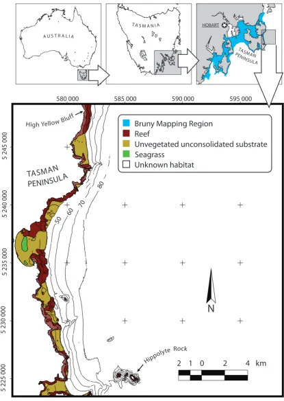
The study area stretched over some 50 km of coastline in south-eastern Tasmania
between High Yellow Bluff and the Hippolyte Rocks (Fig. 2.1). Despite being a
popular recreational SCUBA dive destination, little was known about the benthic
assemblages below diver’s depths (< 30 m). The “Peninsula Mapping Region”
(Barrett et al., 2001) has a dominantely easterly aspect, high vertical cliffs,
deepwater reefs (to 100 m depth) and medium to high wave exposure 2.1. Key
ecological features down to the 40 m depth contour were mapped during the
SEAMAP (www.seamap.imas.utas.edu.au/) project using a range of towed video
surveys Barrett et al. (2001). Geologically the coastline is composed of dolerite,
sedimentary rock and to a lesser extent granite, i.e., the Sisters, see Fig. 2.1 (Barrett
A U S T R A L I A
T A S M A N I A
TASMAN
PENINSULA
High Yellow Blu
ff
Hippol
yte Rock
0 2 4 km
2 1
N
595 000
585 000 590 000
580 000
5 245 000
5 235 000
5 225 000
5 240 000
5 230 000
HOBART
TASMAN
PEN
INSULA
50
60 70
[image:44.595.117.533.95.680.2]80
Figure 2.1: Location of study area (High Yellow Bluff to Hippolyte
Rock). Extent of Bruny Mapping Region (Barrett et al. (2001))
highlighted in blue. Habitats from shoreline to 40 m depth contour
according to www.seamap.imas.utas.edu.au. Depth contours from
2.3
Bathymetric mapping
A ship-borne Simrad EM3002(D) 300 kHz multibeam echo sounder (MBES) in single
transducer mode was used for bathymetric mapping from 13 – 26 June 2008 (Nichol
et al., 2009). The Applanix Position and Orientation system (Applanix Corporation)
collected motion referencing and navigation data. Geographical position during the
survey was recorded using the C-Nav GPS system (C-Nav World DGNSS). Vessel
survey speed in inshore and shallow water areas was 5 knots and 10 knots in deeper
offshore waters. Multibeam data were corrected for tides and vessel motion using
CARIS Hips and Sips v6.1 software (CARIS). The final raster digital elevation model
had a resolution of 2×2 m.
2.4
Autonomous underwater vehicle
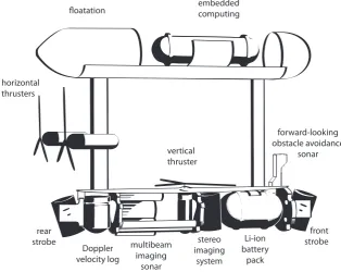
The Autonomous Underwater Vehicle (AUV) Sirius, operated by the Australian
Centre for Field Robotics at the University of Sydney, sampled benthic fauna by
means of digital photography. Sirius was a modified version of the SeaBED AUV
(Singh et al. 2004) built by the Woods Hole Oceanographic Institution (Fig. 2.2).
This ocean-going survey AUV was designed to be passively stable in pitch and
roll. Stability was achieved by two torpedo-like components joined by
turbulence-reducing vertical struts. The upper component consisted of flotation bodies and the
electronics housing, giving the AUV positive buoyancy and the lower component
contained the various sensors and batteries. The overall dimensions of the AUV
on payload, was ∼200 kg. The vehicle was rated to 700 m depth. Yaw, forward
and backward movement was controlled by a pair of aft-facing thrusters. Vertical
(depth) movement was accomplished by one vertical thruster. Geographical vehicle
positioning on the surface was accomplished using GPS. Navigation underwater was
achieved using a Doppler velocity log, inertial measurement unit, ultra-short baseline
acoustic positioning system, pressure sensor and compass. For an exhaustive list of
all vehicle specifications and sensors see Table 2.1. The AUV’s ability to ‘hover’
facilitated a virtually constant altitude of 2 m above the seafloor which equated
to an image footprint of 1.6 × 1.3 m (∼2 m2). Average image area was 2.04 m2
(±0.09 SD). The relatively slow ‘flying’ speed of the AUV is ∼0.4 m/s. A pair of
downward-looking Pixelfly HiRes (1360 ×1024 pixels) digital cameras took images
at a one second interval. Two strobes, one situated at the front and the other at
the back of the AUV, synchronously illuminated the field of view.
2.4.1 AUV camera calibration
The stereo camera setup was calibrated to ensure precise photogrammetric
measurements. Images of an object with known dimension were recorded using
the stereo camera setup in a circular pool filled with seawater. This object was
a printed chequerboard-pattern laminated to a 80 × 80 mm stiff perspex board.
The photogrammetric bundle adjustment package CAL (Seager, 2009c) was used to
derive a set of constants specifying the coordinate system of the stereo camera unit
(datum). The resultant parameters were necessary for photogrammetric length, area
Table 2.1: List of AUV specifications and sensors
Vehicle Specifications
Depth rating 700 m
Size 2.0 m (L) × 1.5 m (H) ×1.5 m (W)
Mass 200 kg, depending on payload
Maximum Speed 1.2 m/s
Batteries 1.5 kWh Li-ion pack
Propulsion 3 ×150 W brushless DC thrusters
Navigation
Attitude/Heading Tilt (±0.5◦), Compass (±2◦)
Depth Paroscientific pressure sensor (0.01 %)
Velocity RDI Navigator ADCP (1 - 2 mm/s)
Altitude RDI Navigator
USBL TrackLink 1500 HA (0.2 m range, 0.25◦)
GPS Ashtech A12
Optical Sensing
Camera Stereo Prosilica 12bit 1360 × 1024 CCD
Lighting 2 ×2.8 J strobe
Separation ∼1 m between camera and strobe
Acoustic Sensing
Multibeam sonar Imagenex DeltaT 837 Profiling 260 kHz
Imaging sonar Tritech Seaking (optional)
Obstacle Avoidance lmagenex 852 Echo Sounder
Other Sensors
CTD Seabird 37SBI
Fluorometers Wetlabs Ecopuck (chlorophylla, CDOM, scattering red)
dissolved oxygen Aanderaa Optode
Communications
Radio Frequency Freewave 900kHz radio + ethernet
embedded computing floatation
rear strobe
front strobe Doppler
velocity log
stereo imaging
system multibeam
imaging sonar
Li-ion battery
pack
forward-looking obstacle avoidance
sonar horizontal
thrusters
[image:48.595.167.482.98.348.2]vertical thruster
Figure 2.2: Labelled schematic of Autonomous Underwater Vehicle
and its components. Note: Top and bottom hull cover removed for clarity.
2009a).
2.4.2 AUV sampling design
The AUV sampled rocky reefs from 6 – 14 October 2008 with the support of R/V
Challenger (Nichol et al., 2009). Total transect length was ∼60 km (16 dives).
Individual AUV dives were haphazardly placed on prominent deep-water rocky reefs
(25 – 100 m depth) emphasising on rocky reefs as well as transition zones between
reef and adjacent sandy areas. Transect placement was based on visual assessments
of sun-illuminated geoTIFF files from a previous multibeam survey (Nichol et al.,
2009). The intersecting survey pattern (Fig. 5.1) was necessary to maintain high
it is anticipated that the AUV is sampling the same transect during each survey.
This survey pattern reduced positional error, introduced by dead-reckoning and
sensor inaccuracies, by using the simultaneous localisation and mapping (SLAM)
technique. SLAM re-navigated the estimated vehicle trajectories (Williams et al.,
2008b) based on matching images (intersections).
2.4.3 AUV image annotation
AUV images were manually annotated, recording habitat type and mobile
megafauna, e.g., fishes, echinoderms, crustaceans and molluscs. Eleven habitat
types in three subgroups, hard and soft substrate and transition zones are described
in Table 2.2. Annotation was based on the dominating (> 50%) visible feature
within the image irrespective whether it is a physical and biological structuring
component. For example, although it is a fair assumption that the macroalga
Ecklonia radiata resides on hard substrate, images containing E. radiata were
classified as ECKLONIA (provided E. radiata cover was > 50%). During habitat
scoring only changes in habitat type were recorded. For example, if image 1 – 100
depicted habitat type sand and image 101 - 120 depicted habitat type high relief
reef, there would be only two records; image 1 - sand, image 101 - high relief reef.
The remaining images, 2 – 100 and 102 – 120, were automatically labelled based
on its predecessor’s label using a MATLAB script. Species identification was based
on identification guides (Gomon et al., 2008; Edgar, 1997) and expert advice from
leading taxonomists. Each image was recorded with a unique date and time stamp.
depth, salinity, temperature, etc.
Table 2.2: Habitat types scored during AUV image annotation with
brief description
habitat type description
Caulerpa macroalgae, Caulerpa spp, covering more
than 50% of the rocky seafloor
Ecklonia macroalga Ecklonia radiata covering more
than 50% of the rocky seafloor
high relief reef rocky reef, elevation change more than 20 cm
(within image)
low relief reef rocky reef, elevation change less than 20 cm
(within image)
coarse sand coarse sand with small pebbles and gravel
pebble and tuft coarse sand with small pebbles and gravel
dominated by bryozoan tuft
sand fine sand
screw shell rubble screw shells, Maoricolpus roseus, covering
more than 50% of the sandy seafloor (within image)
screw shell
rub-ble/sand
screw shells covering less than 50% of the sandy seafloor
patch reef patches of rocky reef within sand
reef-sand ecotone rocky reef edge, transition to/from sand
2.5
Baited underwater video system
Although, underwater photography is almost as old as photography itself (Norton,
2000), baited underwater video systems were first deployed in 1996 by Willis and
Babcock (2000). Their downward-looking (vertical) camera design was subsequently
changed to a forward-looking (horizontal) camera design, culminating in stereo
BUVS pioneered by Harvey and Shortis (1996). BUVS are primarily used to
assess fish assemblage composition. Cappo et al. (2004) found that BUVS sampled
significantly different tropical reef fish assemblages compared to prawn trawls. In
abundance, comparing BUVS with UVC and angling. Several other studies tested
BUVS performance compared to UVC and unbaited underwater video systems
(Langlois et al., 2010; Watson et al., 2005). Watson et al. (2007) found that the
establishment of a marine reserve caused changes in assemblage composition in a
temperate-tropical transition zone. All references above are studies in shallow (<30
m) waters and do not assess fish assemblage compositions below safe SCUBA diving
depths. This study used BUVS to describe benthic fish assemblages in temperate
deep-water (>30 m) rocky reef environments.
2.5.1 BUVS design and components
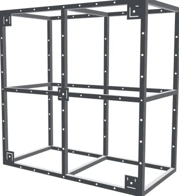
The BUVS frame was shaped like a truncated pyramid with an oblong base. It
consisted of four galvanised steel parts, these were:
(i) the frame base, which besides forming the base of the frame acted as a
redundant safety device. In case of BUVS entanglement, vigorous pulling
detached the base from the top. The top part, consisting of the underwater
housings and cameras, can be retrieved with the minor loss of the base. 6 kg
galvanised steel bars for weighting and balancing the frame can be attached to
all four sides of the frame base.
(ii) the frame top held the camera bar and also provided an attachment point for
the rope.
(iii) the camera bar was designed as an independent unit for ease of camera
made from pressure-pipe PVC with detachable plexiglas front dome and fixed
rear dome were attached to the bar, ∼75 cm apart and inwardly converged by
8° for optimised field of view (Harvey and Shortis, 1996).
(iv) the detachable bait arm was intended to decrease overall unit dimensions and
ease of transport. Whilst one end attached to the camera bar, the outward end
served as an attachment point for the bait basket and LED array. The array
was visible in the video footage of both cameras and the LED blinking sequence
provided a reference to synchronise video footage of the left and right camera.
Synchronisation reduces photogrammetric measurement error by overcoming
motion parallax (Harvey and Shortis, 1996).
A negatively buoyant rope (12 mm diameter) attached to the frame top allowed for
easy BUVS retrieval by hauling with assistance of an electrical winch. Two white
polystyrene surface floats (250 mm diameter) were attached to the end of the rope
to provide flotation and increase visibility from distance. A schematic of the frame
and camera housings is provided in Fig. 2.3.
Underwater camera housings
The tubular camera housings, depth rated to 150 m, were made from pressure-pipe
PVC and plexiglass domes. The detachable front dome connected to an aluminium
frame that served as a base for the video camera. An alignment pin on the front of
Figure 2.3: Schematic of BUVS unit; LED array (green) on bait arm, pins (red) for weight attachment, cameras and underwater housings (blue outline).
Video cameras
Six JVC GZ-MS100 PAL (720×576 pixels) off-the-shelf video cameras, two for each
of the three frames, were used during this study. A Raynox wide angle conversion
lens (conversion factor 0.7) was attached to the cameras to increase the field of view.
Using the higher capacity JVC battery pack (BN-VF823U) increased recording time,
∼4 hours. Video footage was recorded on 16 GB SDHC memory cards.
2.5.2 BUVS camera calibration
Calibrating stereo camera systems ensures precise photogrammetric measurements.
Off-the-shelf cameras are rarely metric and therefore deviate from a perfect central
projection. This deviation needs to be modelled during the calibration process
(for more technical details see Harvey et al. (2003)). Calibrations were conducted
optical properties between seawater and freshwater are negligible with respect to
measurement accuracy (Harvey et al., 2003). Hence calibrations were conducted
in a public swimming pool due to ease of access. An object of known dimensions
(calibration cube) was recorded for later calibration in the video lab. Dimensions of
the precision-made calibration cube were 1 m × 1 m × 0.5 m (Fig. 2.4). The
photogrammetric bundle adjustment package CAL (Seager, 2009c) was used to
derive a set of constants specifying the coordinate system of the stereo camera unit
(datum). The resultant parameters and internal characteristics of the video cameras
such as focal length, principal points, lense distortion, orthogonality and affinity
terms as well as the relative orientation of the two cameras to one another were
necessary for photogrammetric length estimation of objects using the PhotoMeasure
software package (Seager, 2009a).
2.5.3 BUVS sampling design
Bait
BUVS are baited to attract fish to come close to the cameras. Unbaited underwater
video systems record one quarter of the number of individuals recorded by baited
systems (Watson et al., 2005). The de facto standard bait used in BUVS research
is crushed pilchard Sardinops spp. However, Wraith (2007) reports significant
differences in relative abundance and species richness recorded using three different
bait sources, pilchard, abalone and urchin. Although Wraith (2007) studied a
results in Tasmanian waters were non-existent at the time of writing. To find
the most efficient bait source three different baits were tested, crushed pilchard,
crushed salmon and Hook’em Fish Kandy (commercial fish attractant, Hook’em
Fishing). Pilchard was the most effective bait –MaxNfor target species was highest,
biodiversity (species richness and Shannon index) was greatest, time of first arrival
(fish at BUVS station) was shortest and bait plume dispersal period was longest –
and was used for all subsequent BUVS deployments. For each deployment 800 g
of Sardinops sagax was crushed to promote odour dispersal and placed in a plastic
craypot bait basket (Quin Marine Pty Ltd) suspended ∼1 m in front of the two
BUVS cameras. The bait basket was re-filled before each deployment. Replicate
BUVS locations were separated by at least 200 m to prevent overlapping bait plumes.
This would have increased the risk of recording the same individual with two different
BUVS units and therefore inflated relative abundance estimates.
BUVS deployment
BUVS deployment duration differs between temperate and tropical locations
(Watson et al., 2005; Cappo et al., 2004), which is largely attributed to higher
species richness in the latter. Investigations in the tropics require less BUVS
deployment time to record the same number of species compared to investigations in
temperate regions (Cappo et al., 2004). Watson et al. (2005) state that >36 min of
deployment time is necessary to record “the majority of fish species” in temperate
regions of Western Australia. To determine to what extent Watson et al. (2005)’s
of deployment (soak time) and species richness S was investigated during a pilot
study. The pilot study found that at least 40 min of soak time are required to
obtain S as high as the average species richness. Subsequently, soak time at the
bottom was 45 min. BUVS were deployed between 14 May 2009 and 22 August
2010 during daylight hours (8 AM to 6 PM) depending on season using a ∼6 m
boat. Sampling depth ranged from 32 – 81 m. The study area was subdivided
into sites based on distinct reef complexes. These reef complexes were chosen using
a high-resolution bathymetric map obtained during survey leg one. This study
focused on fish assemblages on reef areas with high range values (range: local relief
measure, subtracting the minimum elevation from the maximum elevation in a local
neighbourhood of 6, 10 and 18 m kernel radius); for further details see Moore et al.
(2009). Hence, BUVS were deployed on high relief reef habitats (high range values).
From the moment the BUVS unit is dropped to the moment it reaches the seafloor,
the unit can drift and may not always land in the same geographical position or
habitat. To ascertain that the right habitat was sampled the footage was visually
inspected using the visible camera footprint. BUVS deployments in non-targeted
habitats were discarded. Sampling locations are depicted in Fig. 4.1. Three replicate
samples were taken for each site and each season.
2.5.4 BUVS video annotation
Video footage was viewed and annotated using the software package EventMeasure
(Seager 2009). MaxN, the maximum number of individuals of a given identified
individual (Cappo et al., 2004).
EventMeasure
The software package EventMeasure (Seager, 2008) was used to record species
abundance and diversity as well as fish behaviour by interrogating footage from
the left or right video camera. Every species entering the field of view was recorded
by right-mouse clicking on the individual and choosing the desired attributes (species
name, stage and behaviour). Each of these events was saved to a .emObs file for
later fish length measurements in the software package PhotoMeasure.
Additional information, such as time (frame number) when the BUVS frame hit the
bottom, habitat type, first arrival of first fish and time when the frame was lifted
off the bottom were recorded. MaxN, the maximum number of species x in video
frame y for each 45 min deployment, was used throughout this study to indicate
fish abundance and derive diversity measures such as Simpson’s index (D). MaxNis
considered a relative abundance measure as opposed to a absolute density measure
such as number of individuals of species x per m2. Polymorphic species such as
the blue-throated wrasse Notolabrus tetricus, provided a male and female entered
the field of view, allowed for a different relative abundance measure than MaxN.
For example, if a male and female N. tetricus entered the field-of-view but not at
the same time (video frame y), relative abundance for this 45 min deployment was
2.6
Towed video platform
Geoscience Australia developed small (30 × 50 cm [sic]), shallow-water RayTech
towed interlaced video system consisted of two steel side panels connected by several
rods and bars, that gave stability as well as attachment points for sensors (Fig. 2.5)
(Nichol et al., 2009). A wing on the back of the platform stabilised the ‘flight’ path
(pitch, yaw and roll). A stable platform provides a consistent field of view, i.e., a
consistent sample area. The umbilical cable served as tether and communications
cable to control lights and laser pointers and receive real-time PAL video footage
onboard the support vessel. The two 250 W lights could be switched on and off on
demand but remained off most of the time due to adequate ambient light conditions
and the high sensitivity of the digital video camera. Two laser pointers, 15 cm
apart, underneath the lights served as an indication of scale in the video footage. A
ultra-short baseline system tracked the precise geo-location of the platform during
deployment.
2.6.1 Towed video sampling design
Towed video platform sampling occurred from 25 - 27 February 2009 on R/V
Challenger (Nichol et al., 2009). Video transect length ranged from 200 m to
1.1 km. Transects were conducted in two directions; along depth contours and
across depth gradient. Towed video transects were placed to overlap AUV tracks
and cover roughly the same areal extent for later comparison. The platform was
was controlled by a winch operator, watching the real-time video footage, onboard
the support vessel.
2.6.2 Towed video annotation
Digital video footage with overlaid geographical position was transferred from tape
to hard drive and saved as an AVI-file (Audio Video Interleaved). I used the open
source software package VARS (Video Annotation and Reference Software (Schlining
and Stout, 2006) for viewing and annotation. Mobile invertebrates and vertebrates
were identified to species level where possible based on species identification guides
(Gomon et al., 2008; Edgar, 1997).
VARS
Several data processing steps were required to extract relative abundance and species
richness from the imagery. Video footage taken with the towed video platform was
viewed on a large screen and annotated using MBARI’s open source software package
VARS (Schlining and Stout, 2006). VARS consisted of three parts:
(i) Knowledgebase
(ii) Annotation
(iii) Query
The Knowledgebase consisted of a phylogenetic tree which had to be modified to
the ocean perch, Helicolenus percoidesto the Knowledgebase it was also required to
add its Family, Order, Class, Phylum and Kingdom. VARS Annotation provided
a general user interface to play, pause and stop the digital video file and label
individuals when they occurred in the footage. The resulting record stated time and
videoframe in which a particular individual occurred. Finally, the resulting VARS
Query file enabled the generation of tallies for each species by tow. The hierarchical
phylogenetic tree structure within Knowledgebase allowed for querying other levels
Chapter
3
Image-based continental shelf habitat
mapping using novel automated data
extraction techniques
This Chapter has been accepted for publication and will be printed in Continental
Shelf Research. The manuscript (unformatted and unedited PDF) is now available
online at: http://dx.doi.org/10.1016/j.csr.2012.06.003.
3.1
Abstract
We automatically mapped the distribution of temperate continental shelf rocky
reef habitats with a high degree of confidence using colour, texture, rugosity and
patchiness features extracted from images in conjunction with machine-learning
algorithms. This demonstrated the potential of novel automation routines to
expedite the complex and time-consuming process of seabed mapping. The random
forests ensemble classifier outperformed other tree-based algorithms and also offered
some valuable built-in model performance assessment tools. Habitat prediction using
random forests performed most accurately when all 26 image-derived predictors
were included in the model. This produced an overall habitat prediction accuracy
of 84% (with a kappa statistic of 0.793) when compared to nine distinct habitat
classes assigned by a human annotator. Predictions for three habitat classes were