Time-like reductions of supergravity and black string solutions

(1)

string solutions

Thesis submitted in accordance with the requirements of the University of Liverpool for the degree of Doctor in Philosophy

by Paul Dempster

(2)

Abstract

We consider various geometrical and physical aspects of the supergravityq-maps, which

are induced by dimensional reduction to three dimensions of five-dimensional N = 2

supergravity theories coupled to vector multiplets. In this way, the q-maps can be

thought of as a composition of ther-maps andc-maps. We treat in parallel the case of

reduction over two space-like directions and over one space-like and one time-like

direc-tion. We observe that in the latter case, surprisingly, the order in which the time-like

and space-like reductions are performed is relevant for some geometrical properties of

the resulting reduced theories. For the simplest example of pure supergravity in five

di-mensions, we show indeed that the target manifolds obtained from the two reductions

correspond to inequivalent open submanifolds in the pseudo-Riemannian symmetric

space G₂₍₂₎/(SL2 ·SL2). Moreover, each submanifold is endowed with a different in-tegrable structure which makes one a complex manifold and the other a para-complex

manifold.

As an application we investigate how the q-map can be used to generate new

non-extremal and non-extremal non-BPS static black string solutions in five dimensions. We

also make progress towards constructing new stationary solutions. The generic nature

of these constructions, which don’t rely on the target manifolds being symmetric spaces,

allow us to gain a more systematic understanding of various properties of black objects

in supergravity.

(3)

Declaration

I hereby declare that all work described in this thesis is the result of my own research

unless reference to others is given. None of this material has previously been submitted

to this or any other university. All work was carried out in the Theoretical Physics

Division of the Department of Mathematical Sciences, University of Liverpool, UK,

during the period of October 2010 until April 2014.

(4)

Publication list

This thesis contains material that has appeared in the following publications by the

author:

(1) P. Dempster and T. Mohaupt,“Non-extremal and non-BPS extremal five-dimensional

black strings from generalized special real geometry,” Class. Quant. Grav.31(2014)

045019 [arXiv:1310.5056].

(2) V. Cort´es, P. Dempster and T. Mohaupt,“Time-like reductions of five-dimensional

supergravity,” JHEP04 (2014) 190 [arXiv:1401.5672].

Unpublished material will also be presented, some of which is scheduled to appear in

the following publications:

(3) V. Cort´es, P. Dempster, T. Mohaupt and O. Vaughan, “Special geometry of

Eu-clidean supersymmetry IV: the local c-map,” to appear.

(4) V. Cort´es, P. Dempster and T. Mohaupt,“Time-like reductions of five-dimensional

supergravity with vector multiplets,” to appear.

There are also two publications by the author, completed during the period of the

degree, that will not be presented in this thesis:

(5) P. Dempster and M. Tsulaia, “On the structure of quartic vertices for massless

higher spin fields on Minkowski background,” Nucl. Phys. B865 (2012) 353-375

[arXiv:1203.5597].

(5)

(6) I. L. Buchbinder, P. Dempster and M. Tsulaia,“Massive higher spin fields coupled

to a scalar: aspects of interaction and causality,” Nucl. Phys.B877(2013) 260-289

(6)

Introduction

String theory has long been considered the most likely candidate to provide a consistent

theory of quantum gravity. Since the “second superstring revolution” we have been able

to go beyond string perturbation theory and understand many of the non-perturbative

aspects of string theories, both through various dualities and through the emergence

of the eleven-dimensional theory known as M-theory [1–4]. An important tool in this

regard is provided by supergravity theories, which arise naturally as low-energy effective

theories of string and M-theory.

By considering strings propagating in backgrounds which involve different compact

manifolds, the number of supercharges, as well as the matter content, admitted by the

effective supergravity theories can be varied. An important aspect of such

supergrav-ity theories, which we will make use of throughout this thesis, is the fact that they

come equipped with two types of geometry: spacetime geometry and the geometry of

the scalar target manifold. For theories with 16 or more supercharges (N ≥4 in four

dimensions), the geometry of the scalar manifold is completely fixed once the matter

content of the theory is specified. On the other hand, for theories with 8 or 4

super-charges (N = 2 or N = 1 in four dimensions) the matter content does not completely

fix the scalar geometry, and so such theories can possess a much richer structure.

Whilst the scalar manifolds of N = 1 theories in four dimensions are only required

to be K¨ahler [5], those of the N = 2 theories (which we will concentrate on in this

thesis) must satisfy more restrictive conditions, and are controlled by the properties

(11)

of special geometry. As well as being interesting for purely mathematical reasons [6,

7], such geometry plays an important role in the understanding of non-perturbative

aspects of gauge theories [8, 9], string compactifications [10, 11], and the microscopic

understanding of black hole physics [12–15]. More recently, special geometry has been

used to construct new solutions toN = 8 supergravity [16,17], as well as to obtain new

asymptotically-AdS solutions in gauged supergravities [18–20] with applications to the

AdS/CFT correspondence.

We now present an introduction to the main results in this thesis:

The r-map, c-map and q-map

For the N = 2 supergravity theories in which we will be interested in this thesis one

can understand the effect of both space-like and time-like dimensional reduction via

a series of maps between the target manifolds of such theories: the r-maps [21, 22],

c-maps [23, 24] andq-maps. This latter can be understood as the compositionq=c◦r

of an r-map and a c-map. These maps provide us with important tools both in a

mathematical and physical context, and remain an active area of research.

Mathematically the r-map, c-map, and by extension the q-map, all preserve

com-pleteness [25]. Therefore, by classifying complete projective special real manifolds,

a project initiated in [26], one can obtain large classes of complete, and generically

non-homogeneous, quaternionic-K¨ahler manifolds.

Physically, each of these maps can be understood as a relation between the target

manifolds of two rigid or locally supersymmetric field theories. In this thesis we will be

interested in taking as our starting point a five-dimensional N = 2 theory ofn vector

multiplets.

In the case of rigid supersymmetry, the target manifold of this theory is an affine

special real manifoldMn. By space-like reduction, we obtain a four-dimensional theory

of n vector multiplets, with target space an affine special K¨ahler manifold. A further

space-like reduction gives a three-dimensional theory, for which the degrees of freedom

(12)

Q4n [27]. This provides us with maps

Mn r

−→N2n c

−→Q4n.

If instead one reduces over a time-like direction, then the target manifolds of the

re-sulting Euclidean theories are equipped with a split-signature metric, and can be

de-scribed using para-complex geometry [28, 29]. Indeed, time-like reduction of the

five-dimensional theory gives rise to a target space which is affine special para-K¨ahler [28].

Likewise, both time-like reduction of the four-dimensional Minkowski theory and

space-like reduction of the four-dimensional Euclidean theory give rise to target spaces which

are para-hyperk¨ahler [29].

In the case of local supersymmetry, the target manifold of the five-dimensional

N = 2 supergravity theory with n vector multiplets is a projective special real

mani-fold ¯Mn [30]. By space-like reduction we obtain a four-dimensional theory of (n+ 1)

vector multiplets, the extra degrees of freedom compared to the rigid case coming from

the reduction of the gravity multiplet. The relevant target manifold is a projective

spe-cial K¨ahler manifold ¯N2n+2. A further space-like reduction gives a three-dimensional supergravity theory, for which the degrees of freedom can this time be packaged into

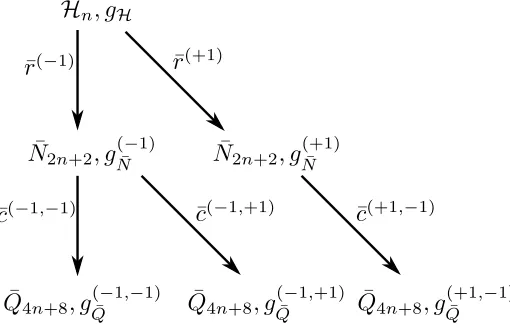
(n+ 2) hypermultiplets, with target space a quaternionic-K¨ahler manifold ¯Q4n+8 [24], as required by supersymmetry [31]. This provides us with maps

¯

Mn

¯

r

−→N¯2n+2 ¯

c

−→Q¯4n+8.

If instead one reduces over a time-like direction, then the target manifolds of the

result-ing Euclidean-signature supergravity theories are again equipped with split-signature

metrics, and can be described using para-complex geometry. Time-like reduction of

the five-dimensional theory gives rise to a target space which is projective special

para-K¨ahler [32].

The study of the time-like versions of the c-map has only been undertaken fairly

recently, in work by the author and collaborators [33, 34]. Here it is shown that both

(13)

of the four-dimensional Euclidean theory give rise to a three-dimensional Eulclidean

theory whose target manifold is para-quaternionic-K¨ahler.

In Chapter 4 we analyse in detail the structure of those (para-)quaternionic-K¨ahler

manifolds which are in the image of one of theq-maps.

Commutativity of space-like and time-like reductions

A central theme throughout this thesis is the use of time-like dimensional reduction as a

solution-generating technique. In particular, instanton solutions to the

dimensionally-reduced Euclidean theories can be dimensionally lifted to provide us with stationary

solitonic solutions, e.g. black holes, to our original supergravity theories [35]. Such

solutions play a crucial role as testing ground for various conjectures in string theory

and other theories of quantum gravity [1].

The structure of Euclidean supergravity theories is much less well understood than

Minkowski-signature ones, and they often present us with surprising features. For

example, in [36] it was shown that time-like reductions of IIA and IIB supergravities

give rise to two inequivalent (i.e. not related by a real field redefinition) nine-dimensional

Euclidean supergravities. This is in contrast to the case of space-like reduction, where

the two nine-dimensional Minkowski theories are related by real field redefinitions:

an artefact of T-duality. One of the primary motivations for this thesis is to better

understand the structure of Euclidean-signature field theories (both with rigid and

local supersymmetry), continuing the work of [28, 29, 32].

An important question that arises in the study of Euclidean supergravity theories

obtained from both space-like and time-like reductions is whether the order of the

reduction matters. In [36] it was argued that, for the case where the scalar manifold

of the Euclidean theory is a homogeneous (coset) space, this order does not matter.

However, their argument rested on being able to parametrise the scalar coset manifold

using the Borel gauge, which for the cosets appearing in Euclidean supergravity theories

(which have non-compact stability group [35]) does not provide aglobal parametrisation

of the manifold.

(14)

super-gravity coupled to an arbitrary number of vector multiplets. Upon reduction to a

three-dimensional Euclidean theory, the scalar target manifolds are generically

non-homogeneous. However, one can use properties of the special geometry underlying

these theories to get a handle on the admissible geometric structures which are present

for all such spaces.

A surprising result of this thesis, which has been presented in a publication by the

author [37], is that, even for the simplest case of pure five-dimensional supergravity,

some of these geometric structures are sensitive to the order in which the space-like

and time-like reductions occur. Note that this is in contrast to the situation for rigid

supersymmetry, where it was shown in [29] that the three-dimensional Euclidean

the-ories obtained by time-then-space (TS) and space-then-time (ST) reductions could be

related by a real field redefinition.

In Chapter 5 we show the two scalar manifolds obtained from TS and ST reduction

of the five-dimensional pure supergravity theory can be distinguished by the existence

of different integrable structures on each. Indeed, for TS reduction, the scalar manifold

comes equipped with an integrable para-complex structure, whilst for ST reduction

we find an integrable complex structure. This fact is generic for all target manifolds

obtained after dimensional reduction of the five-dimensional N = 2 theories to three

Euclidean dimensions, and so this non-commutativity of time-like and space-like

reduc-tions is expected to carry over to the general five-dimensional theory with an arbitrary

number of vector multiplets. This will be analysed further in a future publication by

the author [38].

Black string solutions

In four dimensions, no-go theorems [39] forbid the existence of extended black objects

in general relativity with horizon topology different to S2, which is the case for black holes.

However, higher dimensions are less restrictive, and one can construct solutions

with more exotic horizon topology, see e.g. [40]. The general class of such solutions

(15)

symmetry in some spacetime directions. Such solutions are of particular interest in the

context of string theory.

Such black objects come in two main classes: extremal and non-extremal. These are

distinguished thermodynamically by the fact that extremal black objects have vanishing

horizon temperature. In theories of extended supergravity, extremal objects can be

further separated into BPS and non-BPS. The BPS objects are characterised by the

preservation of some degree of the supersymmetry of their parent theory, and saturate

the Bogomolnyi bound relating their mass to the central charge of the underlying

supersymmetry algebra.

The advantage of studying BPS solutions is that they can be obtained and classified

using the so-called Killing spinor equations [41]. These are a set of first-order

differ-ential equations, and are therefore generally easier to solve than the full second-order

field equations. Such objects are by now well understood, both at a macroscopic and

microscopic level. Constructing non-BPS and non-extremal solutions is significantly

more involved, since these do not satisfy the Killing spinor equations, and as such there

is still a lot to discover.

In this thesis we will concentrate on the case of stationary black strings (1-branes)

in five dimensions. These possess translational symmetry in both a time-like and

space-like direction, which constitute the worldvolume directions of the string. By

dimension-ally reducing over these isometric directions we obtain a three-dimensional

Euclidean-signature supergravity theory, to which we can find instanton solutions. These can then

be lifted back to five dimensions, and to the sought-after black string solutions. This

procedure is generally known as ‘diagonal’ dimensional reduction and oxidation [42].

This dimensional reduction provides us with the link between the spacetime

geome-try and the target space geomegeome-try. In particular, reduction from five to three dimensions

implements the q-map at the level of the target space. All of the five-dimensional

de-grees of freedom then parametrise the para-quaternionic-K¨ahler manifold in the image

of the q-map. In fact, for the static extremal black strings we will meet in Chapter

6, the truncation of certain five-dimensional fields means that we are restricted to a

(16)

Our method for constructing instanton solutions to the three-dimensional Euclidean

theory follows the philosophy of [43], and can be interpreted from the point-of-view of

the target space geometry in the following manner. Single-centred extremal BPS black

strings correspond to null geodesic curves contained within the eigendistributions of

the integrable para-complex structure, whilst non-BPS black strings correspond to null

geodesic curvesnot contained within these eigendistributions. Indeed, we can use such

a geometrical characterisation of extremal solutions whenever the underlying target

manifold admits an integrable para-complex structure. In Chapter 7 we utilise this

fact to construct new BPS and non-BPS stationary solutions for which we relax the

condition of staticity.

The construction of non-extremal solutions is less formulaic. Since non-extremal

black objects are non-BPS, we are unable to use Killing spinor equations. However,

various methods have been used to construct non-extremal black holes and black branes,

which often involve reducing the equations of motion to first-order [44–46].

In Chapter 6, we extend the formalism of [47, 48] and construct non-extremal

solu-tions directly at the level of the equasolu-tions of motion. We first impose that the solusolu-tions

be spherically symmetric in the three-dimensional space transverse to the string. We

are then able to integrate the second-order equations of motion directly and obtain a

general solution, before finding conditions on the integration constants which ensure

that the five-dimensional solutions correspond to physical black strings with finite scalar

fields. These solutions have appeared previously in a publication by the author [49].

This formalism can also be extended to more general non-extremal stationary

solu-tions, and we make progress in this direction in Chapter 7.

Outline

This thesis is organised as follows: in Chapters 2 and 3 we introduce the main

math-ematical and physical background needed to understand the bulk of this thesis. In

Chapter 4 we analyse the supergravity q-maps for the case of an arbitrary number

of vector multiplets coupled to supergravity, and motivate the question of ST vs. TS

(17)

five dimensions, and show that dimensional reduction over one space-like and one

time-like direction provides us with two inequivalent open submanifolds of the symmetric

space G₂₍₂₎/(SL2·SL2). In Chapters 6 and 7 we then turn to spacetime geometry. In Chapter 6 we construct new non-extremal and extremal non-BPS static black string

solutions to five-dimensional supergravity with vector multiplets. Then, in Chapter 7,

we relax the condition of staticity and construct more general stationary solutions. We

finish in Chapter 8 with conclusions and ideas for future work.

Notation and conventions

(18)

Preliminary mathematics

In this chapter we introduce the various mathematical ideas which will be important

throughout this thesis. We begin by simply requiring the existence of a differentiable

manifold, and add further structure (metric, complex structure, quaternionic structure,

etc.) to this as we go.

We begin in Section 2.1 with an overview of differential geometry, introducing the

elementary material upon which the rest of the chapter builds and working up to

special real geometry, which will play an important role in this thesis. In Section 2.2

we introduce the dual notions of complex and para-complex differential geometry, with

the aim of describing projective special (para-)K¨ahler manifolds, before moving on to

discuss (para-)quaternionic-K¨ahler manifolds in Section 2.3. Finally, in Section 2.4, we

turn to the subject of Lie algebras, presenting a number of key results which will be of

use in Chapter 5.

2.1 Differential geometry

In this section we introduce a number of fundamental concepts in differential geometry,

with the aim of familiarising the reader with the tools needed to approach the bulk of

this thesis. We do not claim to give a completely rigorous account of the material, and

refer liberally throughout to the relevant source material for further information.

After some basics, we define in Section 2.1.2 the notion of an (affine) connection

on a differentiable manifold , and use this to discuss geodesy, holonomy and curvature.

(19)

We then equip our manifold with a pseudo-Riemannian metric in Section 2.1.3 and

use this to discuss the Levi-Civita connection, orthonomal frames, pseudo-Riemannian

symmetric spaces, and finish with Berger’s theorem on Riemannian holonomy. We end

with Section 2.1.4 on the subject of special real geometry, which contains many of the

results we will use throughout this thesis.

2.1.1 Basics of differential geometry

Throughout this section we takeM to be some arbitrary m-dimensional differentiable

manifold. We denote by Γ(T M) the set of smooth vector fields on M, i.e. the set of

sections of the tangent bundleT M, and by F(M) the set of smooth functions onM.

Integral curves

Let X ∈ Γ(T M) be some smooth vector field. Then we define an integral curve

generated byX to be a function

γ : [a, b]→M,

parametrized by t ∈ [a, b] such that the tangent to the curve at a point γ(t) ∈ M is

Xγ(t), i.e. the value of the vector field at that point.

In particular, take some local coordinate patch U ⊂M on which we choose a set of

local coordinates{xµ_}_{. Then the integral curve is defined by the property}

dxµ dt =X

µ₍_x₍_t₎₎_. _(2.1)

2.1.2 Connections on the tangent bundle

We now introduce the notion of an affine connection on a differentiable manifold M.

(20)

Affine connections

We define anaffine connection ∇via the map

∇: Γ(T M)×Γ(T M) → Γ(T M)

(X, Y) 7→ ∇XY. (2.2)

In order to be a connection, ∇ must satisfy some properties, namely linearity in its

first argument and the Leibniz identity in its second, viz.

∇f X+gYZ =f∇XY +g∇YZ,

for any X, Y, Z ∈Γ(T M) and f, g∈F(M) some smooth functions on M, and

∇X(f Y) =X(f)Y +f∇XY,

for any X, Y ∈Γ(T M) and f ∈F(M).

Another way of formulating this is via the language of derivations. In particular,

we choose some smooth vector fieldX ∈Γ(T M). Then define a linear map

∇_X : Γ(T M)→Γ(T M),

which acts as a derivation on the module of smooth vector fields Γ(T M) over the ring

of smooth functions F(M). In this context, saying that ∇X acts as a derivation just

tells us that it is linear∇X(Y +Z) =∇XY +∇XZ and satisfies the Leibniz property

as before.

Affine connection in a coordinate basis

Suppose we now choose some coordinate basis forT M, soX =Xµ∂µ. Then

∇_XY = Xµ∇_µ(Yλ∂λ)

(21)

= Xµ

h

∂µYλ+ ΓλµνYν

i

∂λ,

where we have used both linearity (first line) and the Leibniz property (second line) of

the connection. Theconnection coefficientsare defined via.

∇µ∂ν =: Γλµν∂λ,

i.e. they are the components of the vector field∇_µ∂ν in the coordinate basis.

The affine connection on functions

We extend the action of the affine connection ∇_X to the space of smooth functions F(M) onM by

∇Xf =X(f) =£Xf,

where£Xf is the Lie derivative off along the curveX. In a coordinate basisX =Xµ∂µ

we have

X(f) =Xµ ∂f ∂xµ,

which is just the usual directional derivative off along the vector field X.

The affine connection on tensor fields

We can further extend the definition of ∇X to arbitrary rank tensor fields by simply

requiring it to act as a derivation on the algebra of tensor fields D(M) over R. In

particular, we want it to preserve tensor-type (i.e. map tensors of rank (r, s) to tensors

of rank (r, s)), to commute with contractions, and to satisfy

∇X(T1⊗T2) = (∇XT1)⊗T2+T1⊗(∇XT2). (2.3)

As a quick example, we compute the action of∇_X on a smooth 1-formω∈Γ(T∗M). Take some vector field Y ∈ Γ(T M). Then on the one hand the definition of ∇_X on F(M) tells us that we should have

(22)

On the other hand, the property (2.3) tells us that

∇_X(ω(Y)) = (∇_Xω)(Y) +ω(∇_XY),

i.e. the connection acts first on one argument then the other. Putting this together we

find the action of ∇_X on cotangent vector fields to be

(∇Xω)(Y) =X(ω(Y))−ω(∇XY). (2.4)

Parallel transport and geodesics

Choose some smooth vector field V ∈ Γ(T M), and consider the integral curve c(t)

generated byV.

Definition 1. We say that a vector fieldX ∈Γ(T M) isparallel transportedalong

a curve c(t) if

∇VX= 0.

Using this, we define the notion of a geodesic curve γ(t) as an integral curve

generated by a vector fieldV ∈Γ(T M) which satisfies

∇_VV = 0,

at least up to some reparametrization of the curve.

Given a point p ∈ M, we can define the notion of a geodesic symmetry as a

mapsp :M →M which fixespand reverses geodesics throughp, i.e.sp(γ(t)) =γ(−t).

In other words sp(p) = p and (sp)∗ = −1TpM, where (sp)∗ : TpM → TpM is the

differentialofsatp. Note that the mapsp need only be defined in a neighbourhood

of p. Geodesic symmetries will be important later when we talk about symmetric

spaces.

Holonomy

Given a connection ∇ on M, we can use the notion of parallel transport to define a

(23)

In particular, takep∈M and consider the set of all closed loops inM based at p:

Cp(M) ={γ : [0,1]→M|γ(0) =γ(1) =p}.

Now, take a vectorX∈TpM and parallel transport it around some loopc(t)∈Cp(M).

The result will be a new vectorXc∈TpM. Hence, to each loop we can associate a map

Pc:TpM →TpM which takes X7→Xc.

The set of all such transformations, obtained by considering all possible loops in

Cp(M), gives a group Hol(∇, p) ⊂ GL(m,R) called the holonomy group at p.

Ex-plicitly, the action of an element Hol(∇, p) onTpM is given by

PcX=Xh=Xµhµνeν,

whereh∈Hol(∇, p) and {eµ} is a basis of TpM.

Note that if M is arcwise connected, then Hol(∇, p)∼= Hol(∇, q) for anyp, q∈M.

Hence the holonomy group is independent of the base point, and we simply refer to

Hol(∇). This will be the case for all of the manifolds we encounter in this thesis.

Moreover, if we consider only the subset C0

p(M) ⊂ Cp(M) of loops that are

ho-motopic to the identity (can be shrunk to a point) then we obtain the restricted

holonomy group at p, denoted Hol0(∇, p). For simply-connected manifolds this of course coincides with Hol(∇, p).

The torsion tensor

A particularly important tensor field that can be constructed from the affine connection

∇is the torsion tensor

T : Γ(T M)×Γ(T M) → Γ(T M)

(X, Y) 7→ ∇_XY − ∇_YX−[X, Y]. (2.5)

In a coordinate basis {∂_µ} we have

T(X, Y) =

Γλ_µν−Γλ_νµ

(24)

Definition 2. We call an affine connection ∇ torsion-free if T(X, Y) = 0 for any

X, Y ∈Γ(T M).

In terms of a coordinate basis, the torsion-free condition just tells us that the

connection components Γλ_µν are symmetric in their lower indices.

The curvature tensor

Another important tensor field constructed from the connection is thecurvature

ten-sor

R: Γ(T M)×Γ(T M)×Γ(T M) → Γ(T M)

(X, Y, Z) 7→ ∇X∇YZ− ∇Y∇XZ− ∇[X,Y]Z. (2.6)

In a coordinate basis {∂_µ} we have

R(X, Y)Z =XµYνZρ

h

∂µΓλνρ−∂νΓλµρ+ ΓλµσΓσνρ−ΓλνσΓσµρ

i

∂λ.

Definition 3. We call an affine connection∇flatifR(X, Y)Z = 0for anyX, Y, Z ∈

Γ(T M).

Note that for manifolds with flat connection, the holonomy group Hol(∇) is trivial

(see 10.25 of [50]).

2.1.3 Pseudo-Riemannian geometry

We now move on to consider differentiable manifolds endowed with additional structure,

namely the existence of a metric g.

Let (M, g) be a pseudo-Riemannian manifold of signature (p, q). We call an affine

connection ∇ on M metric compatible if ∇g = 0. It turns out that there exists

a unique metric compatible torsion-free connection D on (M, g), which we call the

Levi-Civita connection.

We can compute the Levi-Civita connection explicitly using the Koszul formula [51]

(25)

+g([X, Y], Z)−g(X,[Y, Z])−g(Y,[X, Z]), (2.7)

whereX, Y, Z ∈Γ(T M). Note that when takingX, Y, Z to be coordinate vector fields,

and hence to commute, the final three terms on the right hand side of (2.7) vanish,

and one recovers the usual form of the Levi-Civita connection in terms of Christoffel

symbols. The complementary case, where X, Y, Z are left-invariant vector fields, will

be useful in Chapter 4.

Orthonormal frame

Given a pseudo-Riemannian manifold (M, g), we can define an orthonormal frame

{ea}, which spans T M, satisfying

g(ea, eb) =ηab,

where

ηab=



 

−1p 0

0 1q



 .

We can relate the basis{e_a} to a coordinate basis{∂_µ} by

ea=eaµ∂µ.

The vielbeinseaµ areSL(m,R) matrices and satisfy

eaµebνgµν =ηab,

wheregµν =g(∂µ, ∂ν) are the components of the metricg in the coordinate basis. The

inverse vielbeineµa is given by

eµa=gµνηabebν.

Any two orthonormal frames {e_a} and {e0

a} are related by an SO(p, q)

(26)

orthonormal frames is to introduce a principalSO(p, q) bundle, called theframe

bun-dle, overM [52].

We can define a dual basis {θa_} _of _T∗_M _satisfying _θa₍_e

b) = δba. In terms of the

coordinate basis {dxµ_}_{, we have}

θa=eaµdxµ,

and so the metricg can be written

g=gµνdxµ⊗dxν =ηabθa⊗θb.

For most of the applications in this thesis, it will be convenient to work in such an

orthonormal frame.

Connection 1-form and Cartan’s structure equations

Given an affine connection ∇on a pseudo-Riemannian manifold (M, g), we can write

∇_XY in terms of an orthonormal frame {e_a}, as we did with the coordinate basis in Section 2.1.2. In particular,

∇XY =Xa

eaYc+Ybγabc

ec,

where we have defined the connection coefficients with respect to the basis{ea} as

∇aeb =:γabc ec.

These can be related to the connection coefficients Γρµν of Section 2.1.2 by

γ_abc =eλceaµ

∂µebλ+ebνΓλµν

.

We can likewise write the components of the torsion tensorT and curvature tensor R

(27)

We define the connection 1-formas

ωab =γbca θc. (2.8)

This satisfies Cartan’s structure equations

dθa+ωab∧θb =Ta, (2.9)

dωab+ωac∧ωcb =Rab, (2.10)

where we have defined the torsion 2-form Ta = 1₂T_bcaθb ∧θc, and the curvature 2-form Rab= 1₂Rabcdθc∧θd.

Pseudo-Riemannian symmetric spaces

An important class of pseudo-Riemannian manifolds, which will appear in Chapter 5,

are symmetric spaces. In order to define these, we follow Theorem 10.72 of [50] and

Corollary 8.16 of [53].

Theorem 1. Let (M, g) be a pseudo-Riemannian manifold. Then the following are

equivalent:

(i) DR= 0, where D is the Levi-Civita connection on(M, g).

(ii) The geodesic symmetrysparound any pointp∈M acts isometrically, i.e.(s∗g)p =

gp.

Recall [51] that the pullback(sp)∗ acts on the (0,2) tensor field gas

(s∗g)p(X, Y) =g((sp)∗X,(sp)∗Y), X, Y ∈TpM.

Definition 4. A pseudo-Riemannian manifold satisfying (i) or (ii) in Theorem 1 is

called locally symmetric.

If, in addition, (M, g) is complete and simply-connected, then it is a symmetric

space. In this latter case, the manifold is a homogeneous space1 G/H for which there

1

(28)

exists a certain involutive automorphismσ ofG. In particular, letGσ ={g∈G|σ(g) =

g} be the fixed-point set of the involution, and Gσ

e the component connected to the

identity. Then Gσ_e ⊂H ⊂Gσ. A consequence of this is thatGσ_e, H and Gσ all have the same Lie algebrah. We will have more to say on this in Section 2.4.

Symmetric spaces have an important role to play in the context of extended

su-pergravity theories, as they often turn up as the target manifolds of certain non-linear

sigma models [35]. Indeed, it is in just such a setting that we will meet them in Chapter

5.

Berger’s list of Riemannian holonomies

The notion of holonomy gives rise to a classification of Riemannian manifolds, known

as Berger’s theorem, which will prove illuminating in the remainder of this thesis. We

follow 10.92 of [50].

Theorem 2. Let (M, g) be a Riemannian manifold which is not locally symmetric

and for which the restricted holonomy group Hol0(D) is irreducible2. Then Hol0(D) is contained within one of the groups in Table 2.1.

Holonomy Dimension Manifold

SO(n) n Orientable

U(n) 2n K¨ahler

SU(n) 2n Calabi-Yau

Sp(n) 4n Hyperk¨ahler

Sp(n)·Sp(1) 4n Quaternionic-K¨ahler

G2 7 G2-manifold

[image:28.612.173.426.438.552.2]

Spin(7) 8 Spin(7) manifold

Table 2.1: Berger’s list of Riemannian holonomies

As an example of what Table 2.1 means, we show:

Theorem 3. For a generic orientable Riemannian manifold (M, g) of dimension n,

the holonomy group Hol(D) is contained withinSO(n).

Proof: We first note that, since Dg = 0, the connection D preserves the length of

a vector. Hence, gp(PcX, PcX) = gp(X, X) for any X ∈ TpM. Expanding in an

2

(29)

orthonormal frame {ea} forTpM, we find

ηab =hachbdηcd,

and so h ∈SO(n) ⊂GL(n,R). Hence, the holonomy group is reduced to a subgroup

Hol(D)⊂SO(n).

For the case where M is a (irreducible, simply-connected) symmetric space G/H,

the holonomy group is simply equal to the isotropy subgroupH. This will be important

when we look at the symmetric space G2(2)/(SL2·SL2) in Chapter 5.

Manifolds of special holonomy play an important role in string compactifications

(see [54] and references therein) due to the fact that they admit covariantly constant

spinors (Theorem 3.6.1 of [55]). In particular, this means that strings propagating on a

background including one of these compact manifolds (e.g. heterotic strings onR3,1×X6 whereX6 is a Calabi-Yau threefold [56]) preserve some number of supercharges in the lower-dimensional non-compact space .

2.1.4 Special real geometry

Special real manifolds are central to the main subject matter of this thesis:

five-dimensionalN = 2 supergravity theories. We will see in Chapter 3 that the consistent

supersymmetric coupling of five-dimensional N = 2 vector multiplets with gravity

re-quires the presence of a so-called “projective special real” manifold. In this section

we will introduce the relevant mathematical framework to understand this result. We

follow [48, 57] and unpublished work by V. Cort´es and T. Mohaupt.

We start with an intrinsic definition of a Hessian manifold, and add further structure

until we reach a conic affine special real (CASR) manifold. We then define a projective

special real (PSR) manifold as a certain quotient of, or equivalently a hypersurface in,

the CASR manifold.

Definition 5. A pseudo-Riemannian manifold(M, g,∇)endowed with a flat,

(30)

Given a flat torsion-free connection, ∇, we can cover M with a set of ‘normal

coordinates’hI _{such that the connection components Γ}I

J K vanish. This tells us that

∇XY =XI(∂IYJ)∂J, with ∂I =

∂ ∂hI.

Then the requirement that ∇g be completely symmetric, i.e. that (∇_Xg)(Y, Z) be symmetric in X, Y, Z, can be shown to be equivalent to the condition

∂IgJ K =∂JgIK,

which tells us that locally the metric g can be written as

g= ∂

2_H

∂hI_∂hJ dh

I_⊗_dhJ_,

for someHesse potentialH(h). For the particular case in which the function H is a

cubic polynomial, we have

Definition 6. A Hessian manifold(M, g,∇) with Hesse potential a cubic polynomial

is called an affine special real manifold.

Affine special real manifolds appear in supersymmetric field theory when one wants

to write down a consistent interacting Lagrangian for rigid N = 2 vector multiplets

in five dimensions. In this case, one finds that the scalar fields contained within the

vector multiplets should parametrise an affine special real manifold [28, 58].

Definition 7. A d-conic Hessian manifold (M, g,∇, ξ) is a Hessian manifold (M, g,∇) endowed with a vector fieldξ such that:

(i) Dξ= d₂1, where D is the Levi-Civita connection on (M, g).

(ii) ∇ξ=1.

The first of these conditions can be analysed by recourse to the Koszul formula

(2.7) withY =ξ. The left hand side then reads

(31)

using the first conic condition. Since this is now symmetric in X, Z we need only

concentrate on those terms on the right hand side of (2.7) which are likewise symmetric

inX, Z. Hence, we have

d g(X, Z) =ξg(X, Z) +g([X, ξ], Z) +g([Z, ξ], X),

which in components reads

d gIJ =ξK∂KgIJ +gKJ∂IξK+gIK∂JξK =£ξgIJ. (2.11)

Thusξ acts as a homothety on the metricg.

We turn next to the second condition defining the d-conic Hessian manifold, which

tells us that ∇_Xξ = X for any smooth vector field X ∈ Γ(T M). In terms of special coordinateshI this becomes

XI(∂IξJ)∂J =XJ∂J,

or in other words ∂IξJ =δ_IJ. Hence, the vector field ξ is an Euler vector field

ξ=hI∂I,

with respect to the special coordinates. Plugging this into (2.11) we find

hK∂KgIJ = (d−2)gIJ,

which tells us that the components of the metricg on ad-conic Hessian manifold, with

respect to the special coordinate basis, are homogeneous of degree d−2. Since we

saw already thatgIJ =∂I,J2 H, then the Hesse potential for a d-conic Hessian manifold

should be homogeneous of degree d. Combining this with the definition of an affine

special real manifold, we have

(32)

H(h) =cIJ KhIhJhK for some constants cIJ K.

In the physics literature, CASR manifolds play an important role in moving between

theories with rigid and local supersymmetry. In particular, the additional assumption

that the Hesse potential be homogeneous means that the rigid theory is invariant under

superconformal transformations [57]. One can therefore use the superconformal calculus

in five dimensions [59, 60] to construct a locally supersymmetric theory. Geometrically,

this corresponds to performing the so-called ‘superconformal quotient’, which we now

discuss.

From CASR to PSR manifolds

We start with a CASR manifold (M, g,∇, ξ), which we take to be some domainM ⊂_Rn

parametrized by special coordinates hI, with I = 1, . . . , n. The vector field ξ induces an R+ action onM given by

hI 7→λhI, λ∈R+.

Hence, the domain M should be chosen such that it is invariant under multiplication

by positive numbers.

There are a number of equivalent ways to define a projective special real (PSR)

manifold. The most familiar is to define a PSR manifold as a hypersurface H ⊂ M

given by

H={x∈M|H(x) = 1}.

The full CASR manifold can then be obtained from Hby theR+ action generated by

ξ. We can equip Hwith the metricgH=−1₃g|H, which is assumed to be Riemannian. Away from Hthe tensor field−1

3gon M gives rise to a Lorentzian metric onM, since it is negative definite in the direction of ξ [57].

We can also think ofHas the set of cosets ofM under theR+action. In other words,

we can obtainHby ‘projecting’ along the orbits of the vector field ξ, i.e.H ∼=M/R+.

We now want to equip H with a Riemannian metric. Since £ξg= 3g, we see that

(33)

defineHas a Riemannian coset space, we want a tensor field on M upon whichξ acts

isometrically. To this end, we define

a= ∂

2_H_˜

∂hI_∂hJdh

I_⊗_dhJ_, _where _H_˜ ₌₋1

3logH. (2.12)

One can show that the tensor field a satisfies £ξa= 0, i.e. it is constant along orbits

of ξ. Since it will be useful in Chapter 3, we write explicitly the components of a in

terms of the special coordinates:

aIJ =−2

(ch)IJ

chhh −

3 2

(chh)I(chh)J

(chhh)2

, (2.13)

where we have definedchhh:=cIJ KhIhJhK, (chh)I :=cIJ KhJhK, etc.

We can therefore define a PSR manifold Has the quotient

H ∼=M/R+,

with quotient metric obtained from a. Note that for the hypersurface embedding i :

H →M, the pullback of−1₃g and ainduce the same metric onH:

gH=i∗

−1

3g

=i∗(a).

Projective special real manifolds will be important in Chapter 3, where we will

see that they naturally appear when one tries to consistently couple N = 2 vector

multiplets to gravity in five dimensions.

2.2 (Para-)Complex differential geometry

This section deals in parallel with the subjects of complex and para-complex differential

geometry, which have many important applications in supergravity. Whilst complex

differential geometry is fairly familiar, the use of para-complex differential geometry in

physics was only formalised fairly recently [28]. By introducing the notion of-complex

(34)

manifolds, we are able to treat both types of geometry on the same footing.

The primary aim of this section is to provide the necessary material to understand

projective special -K¨ahler manifolds, which appear in the study of four-dimensional

N = 2 vector multiplets coupled to gravity. However, along the way we will introduce

a host of material which will prove useful throughout this thesis. We begin in Section

2.2.1 by defining almost-complex structures, and treat their integrability in Sections

2.2.2–2.2.3, before moving on in Section 2.2.4 to-K¨ahler manifolds. Finally, the main

bulk of this section is contained in Section 2.2.5 where we introduce the notion of special

-K¨ahler manifolds.

We mostly follow the treatment of [52] for complex geometry, and [28, 32] for its

para-complex cousin.

2.2.1 Almost -complex structure

An -complex structure J is a tensor field such that at each point p ∈ M, the

endo-morphismJp ∈End(TpM) satisfies

J_p2=IdTpM.

For=−1 this is the usual definition of an almost complex structure. For= 1 we also

impose that the two eigenspacesTpM±= ker(Idp∓Jp) have the same dimension [28].

In this caseJ is called an almost para-complex structure.

Given an almost-complex structure J on M, we can define a dual structure J∗ ∈

Γ(End(T∗M)), which is defined by

(J∗ξ)(X) =ξ(J X),

for any ξ∈Γ(T∗M), X ∈Γ(T M).

2.2.2 Integrability of an almost complex structure

We follow Section 2.11 of [50], which gives three equivalent criteria for an almost

(35)

Vector fields

LetZ∈TpMC∼=TpM⊗Cbe a vector in the complexified tangent space at some point

p∈M, and Jp∈End(TpMC) an almost complex structure.

Since Jp is an anti-involution, we can split the complexified tangent space into two

disjoint subspaces [52]

TpMC=TpM+⊕TpM−,

where

TpM±=

n

Z ∈TpMC|JpZ =±iZ

o

. (2.14)

We callTpM+theholomorphic tangent spaceandTpM−theanti-holomorphic

tangent space. These are also sometimes denoted TpM(1,0) and TpM(0,1), which is

the notation we use in the following. Hence, any almost complex structure J gives

rise, at each point p ∈ M, to a decomposition of TpMC into a holomorphic and an

anti-holomorphic tangent space.

We decompose the generators TpMC = span{Xa} into TpM(1,0) = span{Xi} and

TpM(0,1) = span{X¯¯_i}. Then

Definition 9. The almost complex structure J is integrable if [Xi, Xj]∈TpM(1,0)

for anyXi, Xj ∈TpM(1,0).

Since the generatorsXa∈TpMC satisfy the relations

[Xa, Xb] =fabcXc,

the statement that J is integrable is equivalent to the statement that the structure

constantsf_abc satisfy

f_ijk¯ = 0, f¯_ik¯_j = 0. (2.15)

Using this information we can find an equivalent condition for an almost complex

(36)

1-forms

Given the basis {Xa} of TpMC, we can define a dual basis {θa} of the complexified

cotangent spaceT_p∗MC∼₌_T∗

pM⊗Cin the usual way. One can then show [51] that the

θa satisfy

dθa=−f_bca θb∧θc. (2.16)

The decomposition, via J, of TpMCinto a holomorphic and anti-holomorphic

tan-gent space induces a similar decomposition ofT_p∗MC _into_T∗

pM(1,0) and Tp∗M(0,1). We

can then split {θa_} _{into disjoint sets} _{θi_} _and_{_θ_¯¯i_}_.

The exterior derivative decomposes as

dθi =−fi

jkθj∧θk−2fji¯kθ

j_∧_θ_¯¯k₋_fi

¯

j¯kθ¯

¯

j_∧_θ_¯¯k_,

so that J being integrable in the vector field sense given above is equivalent to the

vanishing of the final term here. As such, we have

Theorem 4. The almost complex structure J is integrable in the sense of Definition

9 iff the exterior derivative dθ of any holomorphic 1-form θ ∈ T_p∗M(1,0) contains no (0,2)form.

Newlander-Nirenberg theorem

The final condition for J to be integrable is the subject of the famous

Newlander-Nirenberg theorem. We first define theNijenhuis tensor3

N(X, Y) :=−J2[X, Y] +J[J X, Y] +J[X, J Y]−[J X, J Y]. (2.17)

Then the Newlander-Nirenberg theoremstates:

Theorem 5. The almost complex structure J is integrable in the sense of Definition

9 iff N(X, Y) = 0 for anyX, Y ∈Γ(T M).

The proof can be found in Theorem 8.12 of [52]. Note that the vanishing of the

Nijenhuis tensor is a local condition, so only needs to hold on open sets of M. This

3

(37)

will be important in Chapter 5, when we see that two open orbits contained within the

same pseudo-Riemannian symmetric space admit different integrable structures.

2.2.3 Integrability of an almost para-complex structure

The condition for integrability of an almost para-complex structure can be derived

similarly to the complex case in the previous subsection. However, in this case the

eigendistributionsTpM± are real vector spaces. Since Jp is an involution onTpM, we

can make the decomposition

TpM =TpM+⊕TpM−,

where

TpM±={X∈TpM|JpX=±X}.

Then Frobenius’ theorem guarantees that the almost para-complex structure J is

in-tegrable if [X, Y] ∈ TpM+ for any X, Y ∈ TpM+. Again, this is equivalent to the

condition that the Nijenhuis tensor (2.17) vanishes [28, 61].

The integrability of an almost-complex structureJ defines onM the structure of

an-complex manifold. The simplest examples areCn, whereCis the ring of-complex

numbers

C:=R[i], i2 =.

We call i the -complex unit. For =−1 this is the usual complex unit i, while for

= 1 we have a para-complex unit, generally denoted e. Note that the set of

para-complex numbers is not a field, since it admits zero divisors. Hence, one needs to be

careful when using certain facts from linear algebra. For an overview, see [61].

Note (Proposition 2 of [28]) that a para-complex manifold (M, J) of real dimension

2m is locally a product manifold, so that we can find local coordinates (zi₊, z−i )i=1,...,m

for whichdz±i ◦J =±dz±i . For further details and examples of para-complex manifolds, and para-complex geometry in general, see [62] and references therein.

A function f : M → C is called -holomorphic if df J = idf. This is a

(38)

manifolds (M, J) and (M0, J0), which satisfies df J =J0df.

2.2.4 Almost -hermitian and -K¨ahler manifolds

An almost-complex manifold (M, J) equipped with a pseudo-Riemannian metricgis

said to bealmost -hermitian ifgis compatible with J, i.e.

gp(JpX, JpY) =−gp(X, Y),

for any X, Y ∈ TpM. Then we can define a 2-form ωJ, called the fundamental

2-form, on (M, g, J) via

ωJ(X, Y) =g(J X, Y).

We have

Definition 10. An almost-hermitian manifold(M, g, J) isalmost -K¨ahler if the fundamental 2-formωJ is closed, dωJ = 0.

If J is integrable, then we obtain the usual condition for (M, g, J) to be an

-hermitian or-K¨ahler manifold. In particular, in this case dωJ = 0 can be shown to be

equivalent toDJ = 0, where D is the Levi-Civita connection on (M, g). Then locally

one can find a set of-holomorphic coordinatesza such that the metric g is given by

g= Re

∂2K ∂za_∂_z_¯bdz

a_⊗_d_z_¯b

,

for some functionK(z,z¯) called the -K¨ahler potential.

2.2.5 Special -K¨ahler manifolds

Just as the special real manifolds we met in Section 2.1.4 will prove to be useful for

five-dimensional supergravity theories, so the special K¨ahler manifolds we will introduce

next will be important for the study of four-dimensional N = 2 supergravity theories,

as we will see in Chapter 3.

We begin this section by defining the notion of an affine special -K¨ahler (ASK)

(39)

dimensions. In particular, in order to consistently couple rigidN = 2 vector multiplets

in four-dimensional Minkowski ( =−1) or Euclidean ( = 1) space(time), the scalar

fields should parametrise an affine special -K¨ahler manifold [5, 28].

Definition 11. An-K¨ahler manifold (M, g, J) equipped with a flat torsion-free

‘spe-cial’ connection∇ is called affine special -K¨ahler if:

(i) ∇g is completely symmetric, i.e. (M, g,∇) is Hessian.

(ii) ∇ω= 0, where ω is the fundamental 2-form on (M, g, J).

Since (M, g,∇) is Hessian, we can use the arguments of Section 2.1.4 to introduce a

set of ‘special’ coordinatesXI _on _M_{. The second condition then implies [28] that the}

special coordinates are compatible with the -K¨ahler structure. That is, the metric g

can be obtained from the-K¨ahler potential

K(X,X¯) =i(XIF¯I−X¯IFI), (2.18)

where F(X) is an -holomorphic function called the prepotential. Here we have

used the notation FI(X) =∂IF(X), etc. The components of the metric on the ASK

manifold are then given by4

NIJ(X,X¯) :=

∂2K

∂XI_∂_X¯J =−i FIJ −F¯IJ

. (2.19)

Following the story of special real geometry in Section 2.1.4, we next define a

conic affine special -K¨ahler (CASK) manifold. This plays the same role for the

four-dimensional theory as the CASR manifold did for the five-four-dimensional theory. Namely,

it allows us to move between theories with rigid and local supersymmetry by means of

the superconformal calculus (see [5] and references therein).

Definition 12. A conic affine special -K¨ahler manifold (N, gN, J,∇, ξ) is an

affine special -K¨ahler manifold (N, gN, J,∇) endowed with a vector fieldξ satisfying:

(i) Dξ= Id, where D is the Levi-Civita connection with respect to gN.

4_{Here we write}_N

(40)

(ii) ∇ξ= Id.

Comparing to Definition 7 we see that CASK manifolds are a subclass of 2-conic

Hessian manifolds. We saw there that the vector field ξ was an Euler vector field

with respect to the special real coordinates. Likewise, using special -holomorphic

coordinates XI on N, we find that the conditions (i) and (ii) of Definition 12 imply that

ξ=XI ∂ ∂XI + ¯X

I ∂

∂X¯I. (2.20)

We can also introduce a second privileged vector field J ξ on N, given by

J ξ=iXI

∂

∂XI −iX¯ I ∂

∂X¯I. (2.21)

Together ξ and J ξ generate a C∗ action on the CASK manifold N. In the case

= −1, we see that ξ generates dilatations XI → |λ|XI_{, while} _{J ξ} _{generates a} _U₍₁₎

transformation

XI 7→eiφXI, X¯I7→e−iφX¯I.

In the case= 1,C∗ is the group of invertible para-complex numbers, which is

discon-nected [61]. We can therefore choose whether to allow the full action of C∗=1 ≡ C∗, or just the component connected to the identity C₀∗. Note that the action of e ∈C∗

induces an anti-isometry on the CASK manifold which takesgN 7→ −gN.

Performing an analysis similar to that in Section 2.1.4, we find that ξ acts

homo-thetically ongN, while J ξ acts isometrically

£ξgN = 2gN, £J ξgN = 0.

Moreover, the components (2.19) of the metric gN should be homogeneous of degree

d−2 = 0, which implies that the prepotentialF(X) should be homogeneous of degree

2.

Motivated by analogy with CASR manifolds, we define a tensor field

g= ∂

2_K

∂XI_∂_X¯JdX

(41)

The components of the tensor fieldg are given by

g_I_J¯=− NIJ

XNX¯ +

(NX¯)I(N X)J

(XNX¯)2 , (2.23)

where NIJ are the components of the metric gN on N (2.19). We note that XIgIJ¯=

g_I_J¯X¯J = 0, which implies that the tensor field g is degenerate along the directions spanned by{ξ, J ξ}

g(ξ,·) =g(J ξ,·) = 0.

Hence g does not provide a metric on the CASK manifold. However, both ξ and J ξ

act isometrically ong

£ξg=£J ξg= 0.

Definition 13. A projective special -K¨ahler (PSK) manifold ( ¯N ,g,¯ J¯) is de-fined to be the quotient manifold N/C∗ of a conic affine special -K¨ahler manifold

(N, gN, J,∇, ξ). The metric g¯ on N¯ is induced by the tensor field g on N, while the

-complex structureJ¯onN¯ is induced from J onN.

The C∗ action by which we quotient to get the PSK manifold is that generated

by the vector fields{ξ, J ξ}. Since the tensor field gis isometric along these directions,

it gives a natural metric on the quotient space N/C∗. Note that the action of e∈C∗

mentioned above, which acts as an anti-isometry on the CASK manifold, has no effect

on the metric g of the PSK manifold.

There are a number of ways to think of this construction. It is often convenient

to consider a codimension 1 hypersurface S ⊂ N inside the CASK manifold, given

by gN(ξ, ξ) = const. This fixes the homothety ξ acting on gN and defines a so-called

Sasakian manifold. A particularly useful choice is to consider the hypersurface{K =

1}, where K is the -K¨ahler potential for gN. Since we still have the U(1) action

generated by J ξ, we can then think of the Sasakian manifold S as a U(1) principal

bundle over the PSK manifold ¯N, so ¯N =S/U(1).

The PSK manifold ¯N can be parametrized by a set of projective coordinates

zA= X

A

(42)

Since the prepotential F(X) is homogeneous of degree 2, we write

F(X0, X1, . . .) = (X0)2F

1,X

1

X0, . . .

:= (X0)2F(z1, . . .),

which defines a non-homogeneous prepotential F(z). Using the notation FA := _∂z∂FA,

etc. we can write the metric ¯g on the PSK manifold as

¯

g= Re

∂2K(z,z¯)

∂zA_∂_z_¯B dz

A_⊗_d_z_¯B

, (2.24)

where

K(z,z¯) =−log i

2(F −F¯)−(F_A+ ¯F_A)(zA−z¯A)

. (2.25)

Projective special -K¨ahler manifolds will appear in Chapter 3 when we consider

the coupling of local N = 2 vector multiplets. We will see that our use of a factor

will allow us to treat the case of such theories living in four Minkowski or Euclidean

dimensions simultaneously. Indeed, the coupling of vector multiplets in 3+1 dimensions

will naturally be described by using projective special K¨ahler geometry (=−1), while

in 4 + 0 dimensions they will be described by projective special para-K¨ahler geometry

(= 1).

2.3 (Para-)Quaternionic-K¨

ahler and hyperk¨

ahler

geome-try

In this section we introduce the material necessary for understanding

quaternionic-K¨ahler and hyperk¨ahler geometry. Although fairly complicated mathematically, such

manifolds appear naturally in physics, as we will see in Chapter 3, when one considers

theories of rigid or localN = 2 hypermultiplets.

We first go through some of the preliminaries (Section 2.3.1) for defining

-quaternionic-K¨ahler manifolds. In Section 2.3.2 we define hyperk¨ahler manifolds,

be-fore finishing with (pseudo-)quaternionic-K¨ahler manifolds in Section 2.3.3 and

para-quaternionic-K¨ahler manifolds in Section 2.3.4.

(43)

pre-dominantly [50, 55, 63].

2.3.1 Preliminaries

Symplectic groups

The definitions of hyperk¨ahler and quaternionic-K¨ahler manifolds involve the

symplec-tic groups, as we saw in Table 2.1. We define the symplectic group Sp(2n, F) ⊂

SL(2n, F) over a field F (generally taken to be R or C) to be the group of 2n×2n

matricesM with coefficients inF which satisfy

MTΩM = Ω,

where Ω is the skew-symmetric matrix

Ω = 

 

0 1n

−1n 0



 .

We can use this to define5 thepseudo-unitary-symplectic group Sp(k, l) via

Sp(k, l) =U(2k,2l)∩Sp(2k+ 2l,C)⊂SO(4k,4l).

A particularly useful low-dimensional example is the case k+l= 1, in which case

Sp(2,C) can be identified withSL(2,C), and we see that

Sp(1) =SU(2).

Finally, it will be useful to define a product of the groups Sp(k, l) andSp(1) via

Sp(k, l)·Sp(1) = (Sp(k, l)×Sp(1))/Z2,

where theZ2 factor corresponds to multiplication by±Id. This product has a natural

5

(44)

action on Hm, where m=k+l, via

Sp(k, l)·Sp(1)×_Hm → _Hm

(Aµν, λ;xµ) 7→ Aµνxνλ†,

which makes obvious the action ofZ2 described earlier.

Almost -hypercomplex structures

SupposeM admits two anti-commuting almost complex structures J1, J2, such that

J1J2=−J2J1, J12 =J22=−Id.

Then there is a third almost complex structure J3 = J1J2 with J32 = −Id. In fact, we can define a familyI of almost complex structures onM parametrized by the

two-sphere S2 of unit imaginary quaternions. That is, take ai+bj+ck ∈ Im(H) = S2.

Then

(aJ1+bJ2+cJ3)2=−Id.

The triple{J₁, J2, J3} we call an almost hypercomplex structureon M [64]. Suppose now that M admits an almost complex structure J1 and an almost para-complex structure J2, which anti-commute. Then there exists a second para-complex structure J3 = J1J2. In this case we call the triple {J1, J2, J3} an almost

para-hypercomplex structureon M [65].

Almost -quaternionic manifolds

A manifold M is said to be almost -quaternionic if there exists a sub-bundle Q⊂

End(T M) such that for anyx∈M there exists some open neighbourhoodU 3x such

that

Q|_U = span{J1, J2, J3},

where theJα are a basis of almost-hypercomplex structures on M. We will callQan

(45)

For = −1 this is the usual definition of a quaternionic structure (Section 1.2

of [63]), while for= 1 we call it apara-quaternionic structure [61].

-Quaternionic hermitian manifolds

Let (M, g) be a pseudo-Riemannian manifold such that (M, Q) is an almost

-quaternionic manifold for which the basis of almost -hypercomplex structures are

metric compatible, i.e.

gp(J X, J Y) =−gp(X, Y),

for any X, Y ∈ TpM and J ∈ Qp. Then (M, Q, g) is quaternionic hermitian for

=−1 and para-quaternionic hermitianfor= 1.

2.3.2 Hyperk¨ahler manifolds

We now move on to define hyperk¨ahler manifolds. In the same way that the affine

special real/K¨ahler manifolds which we met earlier encode the couplings of rigidN =

2 vector multiplets, so hyperk¨ahler manifolds encode the couplings of rigid N = 2

hypermultiplets, as we will see in Chapter 3.

As we saw in Theorem 2, the statement that a Riemannian manifold (M, g) be

hyperk¨ahler is a statement about its Riemannian holonomy group. In particular, letD

be the Levi-Civita connection on a 4n-dimensional Riemannian manifold (M, g). Then

Definition 14. (M, g)ishyperk¨ahler if the Riemannian holonomy group Hol(D) is contained within Sp(n).

Note that as Lie groups Sp(n) ⊂ SU(2n) so hyperk¨ahler manifolds represent a

subclass of K¨ahler manifolds. In particular, they are Ricci flat (see Proposition 10.29

of [50]).

Relation to almost complex structures

We can make the relation between hyperk¨ahler and almost K¨ahler manifolds more

(46)

Theorem 6. A Riemannian manifold (M, g) is hyperk¨ahler iff ∃ an almost

hyper-complex structure {J₁, J2, J3} such that (M, g, Jα) is an almost K¨ahler manifold with

respect to each of the Jα.

We can package these conditions into one by defining the quaternion-valued 2-form

ω∈Ω2(M,H) via

ω =iω1+jω2+kω3,

and requiringdω= 0.

This has so far only said that hyperk¨ahler manifolds are almost K¨ahler. However,

there is a theorem by Hitchin (Lemma 1.1.3 of [63]) which tells us that the almost

complex structures Jα are integrable if dω = 0, i.e. if (M, g, Jα) is hyperk¨ahler. The

existence of such a triplet of integrable complex structures in fact makes this a

hyper-complex manifold (Section 7.5.1 of [55]).

Examples

In the casen= 1 we have Sp(1) =SU(2), so a four-dimensional hyperk¨ahler manifold

is K¨ahler and Ricci flat, and vice versa. As such, a compact four-dimensional K¨ahler

manifold with vanishing first Chern class (i.e. a Calabi-Yau 2-fold) is hyperk¨ahler. Such

manifolds are either a torus or aK3 surface.

Non-compact four-dimensional hyperk¨ahler manifolds are important examples of

gravitational instantons, i.e. solutions to the four-dimensional Einstein equations in

Euclidean signature [66, 67].

2.3.3 Quaternionic-K¨ahler manifolds

If we were following directly the discussion of special real and special K¨ahler geometry

above, the natural progression would be to define some notion of “conic-hyperk¨ahler”

manifolds, before taking a superconformal quotient to obtain quaternionic-K¨ahler6 manifolds which could then be used to construct theories of local N = 2

hypermulti-plets.

6_{If we were to continue our naming conventions, these might be called “projective hyperk¨}_{ahler”, but}

(47)

We do not enter into details on this subject, however, as it would remove us too far

from the central narrative. In terms of the superconformal calculus for four-dimensional

hypermultiplets [68], we want to be able to construct a hyperk¨ahler cone, or Swann

bundle [69], over a quaternionic-K¨ahler manifold. This admits a certain H∗ action

which allows us to perform the superconformal quotient as in the real and K¨ahler cases

above. The mathematical details of this procedure goes under the name “QK/HK

correspondence” [70] and is the subject of much recent study [71–76].

As we saw in Theorem 2, the statement that a Riemannian manifold (M, g) be

quaternionic-K¨ahler is a statement about its Riemannian holonomy group. In

partic-ular, let D be the Levi-Civita connection on a 4n-dimensional Riemannian manifold

(M, g) for n≥2. Then

Definition 15. (M, g)is quaternionic-K¨ahler if the Riemannian holonomy group Hol(D) is contained within Sp(n)·Sp(1).

In the casen= 1, we haveSp(1)·Sp(1)∼=SO(4) so any oriented four-dimensional

manifold would automatically be quaternionic-K¨ahler in this sense. However, one

gen-erally applies a more restrictive condition on (M, g) in this case, namely (Section 7.5.1

of [55]):

Definition 16. A four-dimensional Riemannian manifold (M, g) of signature (4,0)

is quaternionic-K¨ahler if it is oriented, Einstein, and has self-dual Weyl tensor.

Relation to quaternionic structure

There is an important theorem (Proposition 14.36 of [50]) which relates the definition of

a quaternionic-K¨ahler manifold given above to the existence of a quaternionic structure

Qon (M, g). In particular

Theorem 7. A Riemannian manifold (M, g) is quaternionic-K¨ahler iff ∃ a

quater-nionic structure Q such that (M, Q, g) is quaternionic hermitian and:

(i) The Levi-Civita connection preserves Q.

Time-like reductions of supergravity and black string solutions

string solutions

Abstract

Declaration

Publication list

Contents

Introduction

Preliminary mathematics

2.1

Differential geometry

2.2

(Para-)Complex differential geometry

2.3

(Para-)Quaternionic-K¨

ahler and hyperk¨

ahler

geome-try