Munich Personal RePEc Archive
The effect of the government
intervention in economy on corruption
Mutascu, Mihai
West University from Timisoara (Romania), Faculty of Economics
and Business Administration
16 June 2009
Online at
https://mpra.ub.uni-muenchen.de/16504/
THE EFFECT OF THE GOVERNMENT INTERVENTION IN ECONOMY
ON CORRUPTION
Mutascu Mihai Ioan, Associate Professor, PhD.
West University of Timisoara, Economic and Business Administration Faculty
Pestalozzi Johan Heinrich16, Timisoara, 300115, Jud. Timis, Romania
Tel: +040-256-592-556, Fax: +040-256-592-500
E-Mail: [email protected], [email protected]
Abstract
The corruption is a complex and generalized phenomenon all over the world, with cultural,
social, psychological, political and economical dimensions. The defining and the studying of the
phenomenon are going through the most different thinking filters known in the specialized
literature: social-cultural, political, administrative and economic. The article’s aim is to quantify
and analyze the relationship between corruption and political, administrative and economic
determinants factors, through a regressive "pool data" model. The sample includes 135 countries
of the world, from all continents, with different degrees of economic development and
political-administrative structures, for the period 1996-2008. What is interesting is that, the study shows
the distortion into the government intervention function in the economy, seen as a significant
proliferation factor for the corruption phenomenon. This connection has different intensity, as the
state is developed, developing or in transition. Moreover, there is a number of unobserved
factors, which emphasizes or temperate in temporal approach the relationship between corruption
- political, administrative and economic determinants factors.
JEL Classification: D73, H10, I30, K20
Keywords: corruption, factors, interventionism, limits, analysis
Acknowledgements: the author wants to thank to the two referees of the Eurasian Journal of
Business and Economics (EJBE) for their precious and constructive observations. Special thanks
to my colleague Bogdan Dima and to the “anonym” person of The William Davidson Institute,
1. Introduction
The corruption is a complex and generalized phenomenon all over the world, with economical,
cultural, social, psychological, political, administrative and religious dimensions. By
consequence, defining and the studying of the phenomenon are going through the most different
thinking filters known in the specialized literature: economic, social-cultural, political,
administrative and religious. In the economic approach, the government controls the distribution
of revenues and the taxation of onerous costs. The private individuals and firms, in such context,
tend to receive the advantages from public authority. If the “payment for advantages” is illegal,
then we can talk about corruption. In an institutional view, for Rose-Ackerman (1999), the
corruption is a symptom for the situations in which the management of the state is inefficient.
All these factors are acting differently, as countries are developed, developing or in transition.
According to Cyper & Dietz (2008), performed over time, it was observed that the developed
economies, with strong industrial sectors and competitive market, have a low level of corruption.
On the opposite side, corruption proliferates in the developing countries and those in transition,
with poorly developed economic sectors and weak competitive markets. Moreover, the factors
intensity can be “accentuated or temperate" temporally under the parallel influence of unobserved
factors, such as: culture, psychosocial individual profile, technological changes, change of
government fiscal policies, natural cataclysms, wars or other internal conflicts.
2. Theoretical fundaments
In the economical view, Shleifer and Vishny (1993) see the corruption as a problem related to the
monopolistic market structure, not a competitive one, and recommend that policies should focus
more closely on the phenomenon of corruption and not on the public sector itself. In a particular
way, Al-Marhubi (2000) finds a significant relationship between inflation and corruption, which
suggests that a high rate of inflation came with a high corruption. For Wang & Rosenau (2001),
the corruption is the secret collaboration between public officials and private actors for private
financial gains in contravention of the public’s interest
Drehel and Schneider (2006) connect the shadow economy with corruption, as an inverse or
general trade policy and fiscal economic equilibrium, Carraro et al. (2006) shows that corruption
affects economic growth with different intensities from one period to another (many studies
refute this results). Moreover, connecting with economic growth, a couple of authors identify and
analyze the inverse relationship between corruption and the level of social welfare. From this
group we regard Svensson (2005).
In the social-cultural sense, Nye (1967) considers the corruption as a deviation from the formal
duties of a public role, in individual compartmental approach: personal, close family and private
clique. The definition summarizes a group of elements, such as bribery, theft, nepotism and
misappropriation. Hungtington (1969) identifies different degrees of corruption, from one culture
to another, with higher intensity in the modernization periods, the corruption being a social
pathology, according to Carvajal (1999).
Husted (1999) describes a cultural profile of a corrupt country as one in which there is high
uncertainty avoidance, high masculinity, and high power distance (without individualism, which
is highly correlated with GNP per capita). Getz & Volkema (2001) revealed that uncertainty
avoidance moderated the relationship between economic adversity and corruption, whereas
power distance and uncertainty avoidance were positively associated with corruption.
Nichols et al. (2004), based on a study that includes two states on different continents, argues that
the corruption perception seeks the recent history of a population, determined by the foreign
domination, the democratic change and the transition periods. Barr and Serra (2006) see the
corruption as a phenomenon set of preferences and rules, following the slogan "not engaging in
bribery because it is harmful to society". They conclude, concise, that the corruption is, in parte, a
cultural phenomenon.
In the political-administrative approach, Hungtington (1969) reveals that the phenomenon of
corruption is an effective absence of the political institutions and Rose-Ackerman (1978) shows
that the decentralization of government decision-making power increases the risk of corruption,
because the review and detection limits are confirmed. Tanzi (1998) accepts the definition of the
World Bank, in which the corruption is the simplest kind of public power abuse for private
benefits, gifts, mainly related to the state monopoly and the way the government perceives the
power. Simply, in a similar way, Rajib and Subarna (2000) develop a general definition of the
bureaucratic apparatus, Drehel and Schneider (2006) show that the better quality of the public
institutions reduces corruption.
In the religious perspective,a previous research has found that religion influences the tendency of
the corruption phenomena. According to Deveterre (2002), the high attention to virtue ethics is
the most effective way to combat corruption. Moreover, religions, such as Christianity, may limit
the effects of this global problem. Particularly, Paldham (2001) founds that the percentage of
Protestants was negatively related to corruption, after controlling for known economic predictors
(real gross domestic product per capita). Several years after, Jude (2004) considers that the
percentage of Protestants within a nation will be negatively related to the level of corruption
within a national economy.
This scientific approach is intended to analyze the relationship between corruption and its
determinant factors of political-administrative and economic nature. According to the mentioned
premise, all the theoretical presented elements allow us to formulate a series of theoretical
working assumptions, which consider two of the approaching coordinates of corruption: one
politico-administrative coordinate and another economical one.
The hypotheses are:
H1: The level of corruption is growing as the civil liberties are less respected; the government
structures and the government intervention in the economy are more extended.
H2: The level of corruption is growing as the social welfare is decreasing.
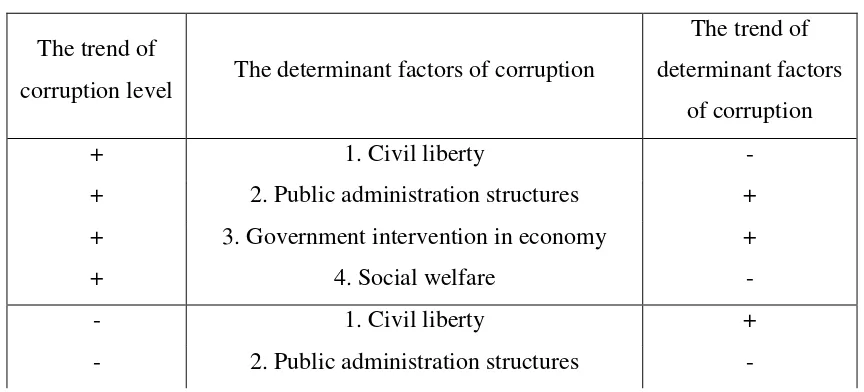
[image:5.612.90.522.513.709.2]In summary, the meanings of the hypothesis’ work relations are:
Table 1: The sense („the sings”) of the hypothesis’ work relations
The trend of
corruption level The determinant factors of corruption
The trend of
determinant factors
of corruption
+ 1. Civil liberty -
+ 2. Public administration structures +
+ 3. Government intervention in economy +
+ 4. Social welfare -
- 1. Civil liberty +
- 3. Government intervention in economy -
- 4. Social welfare +
The fundamental assumption is that corruption is a complex phenomenon determined by a couple
of factors, such as: civil liberties, the administrative government structure, the intensity of state
intervention in economy and the level of social welfare. The linkages are in the same sense for
the case of administrative government structure and the intensity of government intervention and
contrary for the case of civil liberties and social welfare. Moreover, these factors are acting
differently over the time from one type of economy to another and there are a number of
unobserved disturbances.
3. Methods and results
To quantify and analyze the relationship between corruption (dependent variable) and
politico-administrative and economic determinants factors (independent variables), were considered the
period 1996-2008 and a sample of 135 countries of the world, from all continents, with different
degrees of economic development and political-administrative structures. According to Cyper &
Dietz (2008), for a complex approach, the data set was divided into three cross-sectional panels,
as economies are developed - 34 countries, developing - 87 countries and in transition - 14
countries (UNCTAD classification 2009 - Annex). The corruption is quantified by the "Freedom
from corruption” index - FC (the component of the Index of Economic Freedom), developed by
The Heritage Foundation, on a scale from 0 to 100, where 0 indicates a very high level of
corruption and 100 an extremely small one.
The "Civil Liberties" (L) factor is founded by Freedom House - Civil Liberties, the "government
structure" (GS) factor is quantified by The Heritage Foundation - Government Size (the
component of the Index of Economic Freedom) and "social welfare" (HDI) factor is constructed
by the United Nations Development Program - The Human Development Index.
1. The "Civil Liberties" index includes the freedom of expression, assembly, association,
education and religion and has a range of intensity between 1 and 7; the value of 1 is assigned to
the states in which the degree of freedom is very high and 7 to the ones which have a very small
2. The "Government size” index is a component of the "Index of Economic Freedom", which
considers the level of government expenditure as a percentage of GDP, including all levels of
government, such as central/federal, intermediate/state and local level. The scale value is between
0 and 100. The minimum level corresponds to the states which have a small government
spending of GDP, with a reduce redistribution of GDP and government intervention in economy
and vice versa.
3. The "Human Development Index" measures the degree of human development by combining
life expectancy, education levels and realized income, on a scale from 0 to 1, where 0 denotes a
minimum level of welfare and 1 a maximum one.
Because the considered factors have different scales of measurement, for a comparative analysis,
the levels of variables were normalized:
Min Max Max Normalized GS L FC GS L FC GS L FC GS L FC GS L FC , , , , , , , , , , − −
= (1)
[ ]
0,1 ,,L GSNormalized ∈
FC (2)
[ ]
0,1∈
HDI (3)
In this case, for FC - 0 indicates a very high level of corruption and 1 an extremely small one; for
L - 0 is assigned to the states in which the degree of freedom is very high and 1 to the ones which
have a very small one; and for GS - 0 is the minimum level corresponds to the states which have
a small government spending of GDP and 1 to the ones which have a high government spending
of GDP.
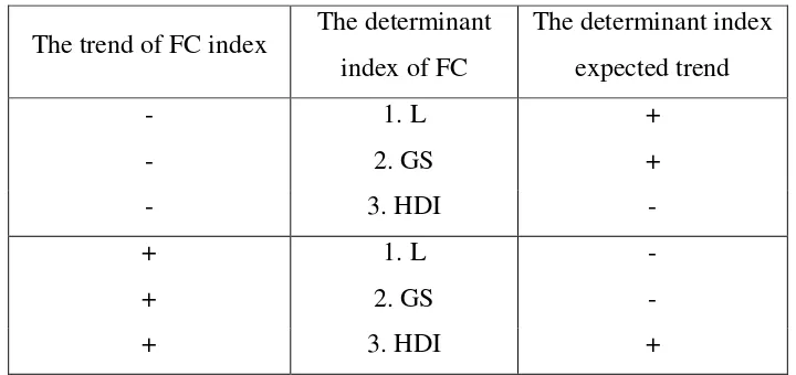
Based on the normalized illustrated variables, the sense of changes existing between corruption
Table 2: The expected sense („the sings”) of the relations between FC - L, GS and HDI,
according to working hypothesis
The trend of FC index The determinant index of FC
The determinant index
expected trend
- 1. L +
- 2. GS +
- 3. HDI -
+ 1. L -
+ 2. GS -
+ 3. HDI +
The method of analysis used is the econometrical modeling (with software EViews 5.0),
elaborating three “Pool Date”1 regressive models, with time-fixed effects, one for each type of
economy, with this shape:
ij t it
it
xX
v
Y
=
+
+
+
(4)where Yit represents the dependent variable - FC, intercept term, independent variables
coefficients, Xit independent variable - L, GS and HDI, t time-varying intercept (captures all of
the variables that affect Yit and that vary over time but are constant cross-sectionally),vij the
remainder disturbance (capturing everything that is left unexplained about Yit), i cross-sectional
units observed for dated periods - (the number of states) and t the period of time (years
1996-2008).
With dummy variables, the model could be:
ij t T t
2 t 1 it
it
xX
xD1
xD2
...
xDT
v
Y
=
+
+
+
+
+
(5)where D1 represents the dummy variable that takes the value 1 for the 1996 year and 0 elsewhere,
and so on.
Finally, the model becomes:
1
it 2008 T
1996 it
3 it 2 it 1
it
xL
xGS
xHDI
xD
...
x
D
v
FC
=
+
+
+
λ
1+
+
λ
+
(6)For testing of three models, I corrected both period heteroskedasticity and general correlation of
observations (except the second model, only with heteroskedasticity correction) within a given
cross-section because the observations are not equal weight in estimation. Moreover, to obtain the
robust coefficient standard errors I applied the Period SUR (PCSE) method.
The econometric analysis of three type economy has two steps:
a. The econometric tests of the „pool data” time-fixed effects models.
b. The “unit root test” of the residuals.
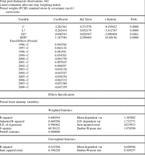
a. The econometric tests of the „pool data” time-fixed effects models, for each type of
economies, are presented in Appendix, Tables A1-A3.
For all type of economies, the tests of models show the following:
- the absolute values of the standard errors corresponding to the coefficients of the function are
lower than the values of the coefficients, witch sustains the correct estimation of these
coefficients (a conclusion reinforced by the low values of the probabilities);
- the value of the correlation coefficient, shows a significant statistical correlation between the
dependent variable - FC and the independent variables - L, GS and HDI (the changes in the FC
are reflected considerably in the changes of L, GS and HDI);
- the value of F-statistic is bigger then the F-critical value (the probability is almost 0), showing
that the model is relevant;
- the Durbin-Watson test (with a resulting value under the critical point of 2) shows that the
residual variables are not autocorrelated.
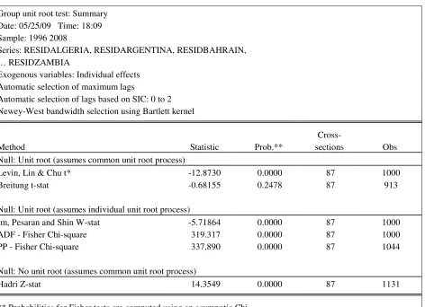
b. The “unit root test” of the residuals. For verifying the stationarity of the residuals are used
the „unit root tests” proposes by Levin, Lin & Chu, Breitung t-stat, Im, Pesaran & Shin W-stat,
ADF, PP and Hadri Z-stat. The results are illustrated in Appendix, Tables A4-A6.
For the developed and developing economies the tests Levin, Lin & Chu; Im, Pesaran & Shin
W-stat; ADF and PP indicate that the null hypothesis is rejected (except Hadri Z-stat test and,
partially, the Breitung t-stat), meaning that the „residuals of the cross-sectional group” is
At limit, for economies in transition, the tests Levin, Lin & Chu; the Breitung t-stat; Im, Pesaran
& Shin W-stat; ADF and PP indicate that the null hypothesis of the unit root can be rejected
(except Hadri Z-stat test).
In conclusion, all three models may be considered representative to describe, at international
level, the connection between FC and L, GS & HDI.
4. Discussion
The obtained results based on the three constructed models show that corruption is mainly the
result of political-administrative and economic factors. The main information can be summaries
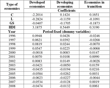
[image:10.612.118.495.360.660.2]in this way:
Table 7: The main results of relationship between “FC-L, GS and HDI”
in the case of Developed economies, Developing economies and Economy in Transition
Developed economies
Developing economies
Economies in transition Type of
economies
Coefficients
C -2.2014 0.1424 0.1651
L -0.2824 -0.1159 -0.1091
GS -0.0407 -0.1705 -0.1873
HDI 3.1875 0.5449 0.3190
Year Period fixed (dummy variables)
1996 0.0948 0.0426 -0.0246
1997 0.0621 0.0392 -0.0268
1998 0.0819 0.0244 -0.0070
1999 0.0547 0.0225 -0.0068
2000 -0.0018 0.0083 0.0147
2001 0.0070 0.0108 0.0090
2002 0.0083 0.0149 -0.0026
2003 -0.0421 -0.0050 0.0159
2004 -0.0435 -0.0194 0.0216
2005 -0.0584 -0.0262 0.0031
2006 -0.0623 -0.0227 -0.0044
2007 -0.0534 -0.0128 0.0019
2008 -0.0474 -0.0132 0.0061
All three elaborated models confirm the proposed theoretical hypotheses, following the idea that
(maximizing L index), the extension of public administration structures, the augmentation of
government intervention in economy (maximizing GS index) and the damage of social welfare
(minimizing HDI index).
In other words, the corruption is high, if the civil liberties are reduced, the structure of
government is extended, the government intervention in the economy is increased and the social
welfare is decreased. Per a contrario, the corruption is low, if the civil liberties are higher, the
structure of government is reduced, the government intervention in the economy is decreased and
the social welfare is increased.
These influences are different intensity as the economies are developed, developing or in
transition. More, there are other several disturbing unobservable factors, with constant and
periodic action. The periodic factors act on the corruption differently, from one year to another,
in positive or negative sense, but they have very little effect on corruption (the impact is less than
10% annually).
In the developed economies the main factor of corruption is the social welfare, followed by civil
liberties, government structure and intensity of the state intervention in economy. In developing
economies and economies in transition the corruption depends mainly on the social welfare, then
on the state intervention in economy and civil liberties.
On this basis, a low level of corruption is assimilated to developed economies, with high life
expectancy, strong literacy and educational attainment and high level of GDP per capita. In this
country people have freedoms of expression and belief, associational and organizational rights
and personal autonomy without interference from the state. Moreover, the bureaucratic structures
are less extensive and state intervention in economy is more temperate, encouraging the private
initiative and market competition rules.
Unfortunately, in the developed economies there are significant unobserved factors that
constantly stimulate corruption, but also there is a set of unobserved factors with periodical
positive or negative actions, with insignificant influence.
A high level of corruption is characteristic for developing economies or economies in
transition, because the life expectancy is low, the degree of literacy and education is precarious
and the level of GDP per capita is low. In addition, freedoms of expression and belief are low,
associational and organizational rights limited and personal autonomy has strong interference
In these economies the state has developed an excessive bureaucratic structure and the state’s
corrective intervention in economy determines often distortions and inefficiencies in the resource
allocation.
In contrast to developed economies, in the developing economies and the economies in transition
the constant unobserved factors have a major destructive influence on corruption. Similarly, the
unobserved factors with periodical acting have an insignificant positive or negative influence.
5. Conclusions
As a complex phenomenon, the corruption hits the entire world, regardless of the geographical
location, population, level of economic development, political regime or type of government.
There are two categories of factors that influence the corruption: some are observed and have
constant periodic influence (social welfare, civil liberties, government structure and intensity of
the state intervention in economy), while others factors are unobserved, with stimulative or
nonstimulative, constant or periodic influences.
Main observable factors act differently as the economies are developed, developing or in
transition.
In the developed economies the most important factor is the level of social welfare, followed by
civil liberties and government size. In other economies, social welfare is followed by the
government size, not by civil liberties. In addition, all these factors are "corrected" by a set of
unobservable influences, positive or negative, with constant or periodic acting.
In such conditions, the improvement of corruption phenomenon is difficult to undertake.
However, based on the described results, we believe that the corrective measures of corruption
must be identified and divided in two categories: one for the developed economies and other for
the developing and economies in transition.
a. The improvement of corruption in developed economies must be focused mainly on the
public health system efficiency (maximizing life expectancy) and the consolidation of
educational system (maximizing the degree of literacy and the level of educational attainment).
A second action, in order of importance, is strengthens of all freedoms of expression and belief,
In the developed economies, the extension of bureaucracy and the state intervention in economy
may be adjusted from a minimum level of efficiency to a maximum level, which corresponds to
the point where they exceed the degree of social welfare and civil liberties.
A great attention should be paid in these economies on unobserved factors that have a strong,
stimulative and constant influence on corruption and exceed the positive unobserved periodical
factors (period dummy). Therefore, regarding corruption, the countries with developed
economies have a high sensitivity to certain nonperiodical factors.
b. The improvement of corruption in developing economies and economies in transition
must be focused preponderant on the public health reforms (increase of the life expectancy level)
and the reconstruction of the educational system (positive effect on degree of literacy and level of
educational attainment).
A second step should be polarized on compression of the bureaucracy structures, the increase of
the bureaucratic professionalism and performance and implementation of the measures to correct
the market allocations, distribution and stabilization. Moreover, the state must "cement" the
private initiative and the market competition rules.
Not least, these countries must make serious efforts to strength democracy, respecting the
freedoms of expression and belief, associational and organizational rights and personal autonomy
toward state.
A big advantage of developing and in transition economies is given by unobserved nonperiodical
factors that have a small but destructive influence on corruption (highest in the transition
economies). Moreover, these constant factors counteract successfully the unobserved temporal
negative factors.
In conclusion, we can appreciate that the improvement measures of corruption phenomenon
should be adapted as economies are developed, developing or in transition. Moreover, in a state
with developed economy a great attention must be focused on the unobserved constant factors,
these types of economies showing a high sensitivity in this sense.
The main results suggest that the corruption is a “key question” especially in developing and in
transition economies, but the disturbance constant unobserved factors decrease the phenomenon
References
Al-Marhubi F (2000) Corruption and inflation. Economics Letters 66
Carraro A, Fochezatto A, Hillbrecht O (2006) O Impacto Da Corrupção Sobre O Crescimento
Econômico Do Brasil: Aplicação De Um Modelo De Equilíbrio Geral Para O Período 1994-1998.
Anais do XXXIV Encontro Nacional de Economia.Proceedings of the 34th Brazilian Economics
Meeting No.57
Carvaja R (1999) Large-Scale Corruption: Definition, Causes, and Cures. Systemic Practice and
Action Research, Vol. 12 (4)
Cypher J, Dietz J (2008) The Process Of Economic Development 3rd Edition. Hardcover Press
Barr A, Serra D (2006) Culture and Corruption. Centre for the Study of African Economies,
University of Oxford, March 1
Devettere R (2002) Introduction to Virtue Ethics, Boulder, Lynne Rienner Co.
Drehel A, Schneider F (2006) Corruption and the Shadow Economy: An Empirical Analysis.
CESIFO Working Paper No. 1653, Category 1: Public Finance
Hofstede G (2003) Culture’s Consequences, Comparing Values, Behaviors, Institutions, and
Organizations Across Nations. Sage Publications, Second Edition
Hungtington S (1968) Modernization and corruption, Political Order in Changing Societies. New
Haven. Conn., Yale University Press
Husted B (1999) Wealth, Culture, and Corruption. Journal of International Business Studies,
Vol.30, No. 2, (2nd Qtr., 1999)
Nichols P, Siedel G, Kasdin M (2004) Corruption as a Pan-Cultural Phenomenon: An Empirical
Study in Countries at Opposite Ends of the Former Soviet Empire. 39 Tex. Int'l L.J. 215
Nye J (1967) Corruption and Political Development: A Cost-Benefit Analysis. 61 American
PoliticalScience Review 417, 419
Paldham M (2001) Corruption and religion: Adding to the economic model. Kyklos 54
Rajib N, Subarna K (2000) Corruption Across Countries: The Cultural and Economic Factors.
Business & Professional Ethics Journal, Vol. 21 (1)
Rose-Ackerman S (1999) Corruption and Government: Causes, Consequences, and Reform.
Cambridge University Press
Shleifer A, Vishny R (1993) Corruption. Quarterly Journal of Economics. Vol. 108 (3)
Svensson J (2005) Eight Questions about Corruptions. Journal of Economic Perspectives (19)
Tanzi V (1998) Corruption Around the World: Causes, Consequences, Scope, and Cures. IMF
Working Paper No. WP/98/63, Washington, May
Wang H, Rosenau J (2001) Transparency International and Corruption as an Issue of Global
Governance.Global Governance 7(1)
Tanzi, V. (1998) „Corruption Around the World: Causes, Consequences, Scope, and Cures”, IMF
Appendix
Table A1:The econometric tests of the „pool data” time-fixed effects model
FC-L, GS and HDI - Developed economies
Dependent Variable: FC?
Method: Pooled EGLS (Period SUR) Date: 05/23/09 Time: 18:09 Sample: 1996 2008
Included observations: 13 Cross-sections included: 34
Total pool (balanced) observations: 442
Linear estimation after one-step weighting matrix
Period weights (PCSE) standard errors & covariance (no d.f. correction)
Variable Coefficient Std. Error t-Statistic Prob.
C -2.201361 0.271578 -8.105822 0.0000 L? -0.282434 0.052179 -5.412787 0.0000 GS? -0.040743 0.020367 -2.000468 0.0461 HDI? 3.187540 0.298404 10.68196 0.0000 Fixed Effects (Period)
1996--C 0.094760 1997--C 0.062134 1998--C 0.081941 1999--C 0.054703 2000--C -0.001758 2001--C 0.007019 2002--C 0.008297 2003--C -0.042120 2004--C -0.043547 2005--C -0.058358 2006--C -0.062332 2007--C -0.053380 2008--C -0.047359
Effects Specification
Period fixed (dummy variables)
Weighted Statistics
R-squared 0.680544 Mean dependent var 1.385802 Adjusted R-squared 0.669296 S.D. dependent var 1.732771 S.E. of regression 0.996462 Sum squared resid 422.9913 F-statistic 60.50123 Durbin-Watson stat 1.978590 Prob(F-statistic) 0.000000
Unweighted Statistics
Table A2:The econometric tests of the „pool data” time-fixed effects model
FC-L, GS and HDI - Developing economies
Dependent Variable: FC?
Method: Pooled EGLS (Cross-section weights) Date: 05/23/09 Time: 18:09
Sample: 1996 2008 Included observations: 13 Cross-sections included: 87
Total pool (balanced) observations: 1131 Linear estimation after one-step weighting matrix
Period weights (PCSE) standard errors & covariance (no d.f. correction)
Variable Coefficient Std. Error t-Statistic Prob.
C 0.142492 0.020791 6.853494 0.0000 L? -0.115900 0.011634 -9.962188 0.0000 GS? -0.170513 0.019265 -8.851125 0.0000 HDI? 0.544997 0.016274 33.48911 0.0000 Fixed Effects (Period)
1996--C 0.042580 1997--C 0.039202 1998--C 0.024439 1999--C 0.022467 2000--C 0.008307 2001--C 0.010848 2002--C 0.014932 2003--C -0.004954 2004--C -0.019449 2005--C -0.026229 2006--C -0.022748 2007--C -0.012767 2008--C -0.013192
Effects Specification
Period fixed (dummy variables)
Weighted Statistics
R-squared 0.740736 Mean dependent var 0.437109 Adjusted R-squared 0.737248 S.D. dependent var 0.308896 S.E. of regression 0.158338 Sum squared resid 27.95410 F-statistic 212.3757 Durbin-Watson stat 1.960999 Prob(F-statistic) 0.000000
Unweighted Statistics
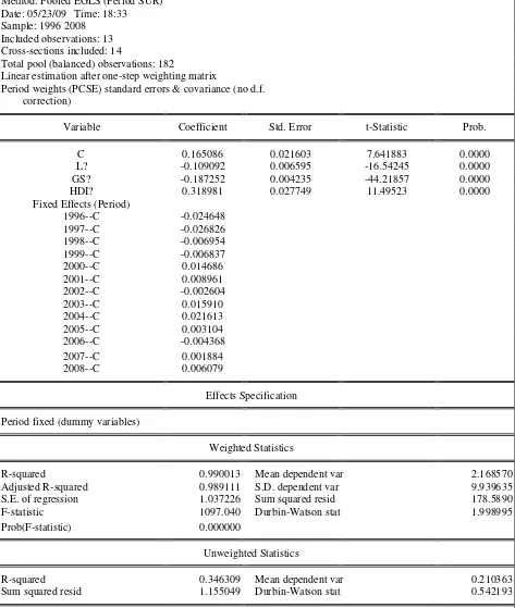
Table A3:The econometric tests of the „pool data” time-fixed effects model
FC-L, GS and HDI – Economies in transition
Dependent Variable: FC?
Method: Pooled EGLS (Period SUR) Date: 05/23/09 Time: 18:33 Sample: 1996 2008
Included observations: 13 Cross-sections included: 14
Total pool (balanced) observations: 182
Linear estimation after one-step weighting matrix
Period weights (PCSE) standard errors & covariance (no d.f. correction)
Variable Coefficient Std. Error t-Statistic Prob.
C 0.165086 0.021603 7.641883 0.0000 L? -0.109092 0.006595 -16.54245 0.0000 GS? -0.187252 0.004235 -44.21857 0.0000 HDI? 0.318981 0.027749 11.49523 0.0000 Fixed Effects (Period)
1996--C -0.024648 1997--C -0.026826 1998--C -0.006954 1999--C -0.006837 2000--C 0.014686 2001--C 0.008961 2002--C -0.002604 2003--C 0.015910 2004--C 0.021613 2005--C 0.003104 2006--C -0.004368 2007--C 0.001884 2008--C 0.006079
Effects Specification
Period fixed (dummy variables)
Weighted Statistics
R-squared 0.990013 Mean dependent var 2.168570 Adjusted R-squared 0.989111 S.D. dependent var 9.939635 S.E. of regression 1.037226 Sum squared resid 178.5890 F-statistic 1097.040 Durbin-Watson stat 1.998995 Prob(F-statistic) 0.000000
Unweighted Statistics
Table A4: The “unit root test” of the residuals - Developed economies
Group unit root test: Summary Date: 05/23/09 Time: 18:54 Sample: 1996 2008
Series: RESIDAUSTRALIA, RESIDAUSTRIA, RESIDBELGIUM, … RESIDUNITEDSTATES
Exogenous variables: Individual effects Automatic selection of maximum lags
Automatic selection of lags based on SIC: 0 to 2 Newey-West bandwidth selection using Bartlett kernel
Cross-
Method Statistic Prob.** sections Obs Null: Unit root (assumes common unit root process)
Levin, Lin & Chu t* -10.9395 0.0000 34 389 Breitung t-stat -0.29030 0.3858 34 355
Null: Unit root (assumes individual unit root process)
Im, Pesaran and Shin W-stat -8.18247 0.0000 34 389 ADF - Fisher Chi-square 191.506 0.0000 34 389 PP - Fisher Chi-square 199.824 0.0000 34 408
Null: No unit root (assumes common unit root process)
Hadri Z-stat 8.56268 0.0000 34 442
Table A5: The “unit root test” of the residuals - Developing economies
Group unit root test: Summary Date: 05/25/09 Time: 18:09 Sample: 1996 2008
Series: RESIDALGERIA, RESIDARGENTINA, RESIDBAHRAIN, … RESIDZAMBIA
Exogenous variables: Individual effects Automatic selection of maximum lags
Automatic selection of lags based on SIC: 0 to 2 Newey-West bandwidth selection using Bartlett kernel
Cross-
Method Statistic Prob.** sections Obs Null: Unit root (assumes common unit root process)
Levin, Lin & Chu t* -12.8730 0.0000 87 1000 Breitung t-stat -0.68155 0.2478 87 913
Null: Unit root (assumes individual unit root process)
Im, Pesaran and Shin W-stat -5.71864 0.0000 87 1000 ADF - Fisher Chi-square 319.317 0.0000 87 1000 PP - Fisher Chi-square 337.890 0.0000 87 1044
Null: No unit root (assumes common unit root process)
Hadri Z-stat 14.3549 0.0000 87 1131
Table A6: The “unit root test” of the residuals - Developing economies
Group unit root test: Summary Date: 05/23/09 Time: 19:06 Sample: 1996 2008
Series: RESIDARMENIA, RESIDAZERBAIJAN, RESIDGEORGIA, … RESIDMACEDONIA, RESIDUKRAINE
Exogenous variables: Individual effects Automatic selection of maximum lags
Automatic selection of lags based on SIC: 0 to 2 Newey-West bandwidth selection using Bartlett kernel
Cross-
Method Statistic Prob.** sections Obs Null: Unit root (assumes common unit root process)
Levin, Lin & Chu t* -2.98818 0.0014 14 164 Breitung t-stat -1.41211 0.0790 14 150
Null: Unit root (assumes individual unit root process)
Im, Pesaran and Shin W-stat -1.25651 0.1045 14 164 ADF - Fisher Chi-square 33.0172 0.2351 14 164 PP - Fisher Chi-square 42.5182 0.0387 14 168
Null: No unit root (assumes common unit root process)
Hadri Z-stat 4.57709 0.0000 14 182
Annex
ElSalvador Namibia UnitedArabEmirates Netherlands EquatorialGuinea Nepal Uruguay NewZealand Developing
economies
Ethiopia Nicaragua Venezuela Norway Algeria Gabon Niger Vietnam Poland Argentina Ghana Nigeria Yemen Portugal
Bahrain Guatemala Pakistan Zambia Romania Bangladesh GuineaBissau Panama Developed
economies
Slovakia
Belize Haiti Paraguay Australia Slovenia Benin Honduras Peru Austria Spain Bolivia India Philippines Belgium Sweden Botswana Indonesia Rwanda Bulgaria Switzerland
Brazil Iran Samoa Canada UnitedKingdom BurkinaFaso Jamaica SaudiArabia Cyprus UnitedStates
Burundi Kenya Senegal CzechRepublic Economies in transition Cambodia Kuwait Singapore Denmark Armenia Cameroon Lao SouthAfrica Estonia Azerbaijan CapeVerde Lesotho SriLanka Finland Georgia CentralAfrican Libyan Sudan France Kazakhstan
Chad Madagascar Suriname Germany Kyrgyzstan Chile Malawi Swaziland Greece Tajikistan China Malaysia Syria Hungary Uzbekistan Colombia Mali Tanzania Iceland Albania
Congo Mauritania Thailand Ireland Belarus CongoDemocratic Mauritius Togo Italy Croatia CostaRica Mexico TrinidadTobago Japan Moldova DominicanRepublic Mongolia Tunisia Latvia Russia