A comparative study on global wavelet and polynomial models for nonlinear regime-switching systems

promoting access to White Rose research papers

White Rose Research Online

Universities of Leeds, Sheffield and York

http://eprints.whiterose.ac.uk/

This is an author produced version of a paper published in

International Journal

of Modelling Identification and Control.

White Rose Research Online URL for this paper:

http://eprints.whiterose.ac.uk/8549/

Published paper

Wei, H.L and Billings, S.A (2007)

A comparative study on global wavelet and

polynomial models for nonlinear regime-switching systems.

International Journal

of Modelling Identification and Control, 2 (4). pp. 273-282.

A prepublication draft of the paper published in

International Journal of Modelling, Identification and Control, Vol. 2, No.42, pp.273-282, 2007.

A Comparative Study on Global Wavelet and Polynomial Models

for Nonlinear Regime-Switching Systems

Hua-Liang Wei and Stephen A. Billings

Department of Automatic Control and Systems Engineering, University of Sheffield Mappin Street, Sheffield, S1 3JD, UK

[email protected], [email protected]

Abstract—A comparative study of wavelet and polynomial models for nonlinear regime-switching (RS) systems is carried out. Regime-switching systems, considered in this study, are a class of severely nonlinear systems, which exhibit abrupt changes or dramatic breaks in behavior, due to regime switching caused by associated events. Both wavelet and polynomial models are used to describe discontinuous dynamical systems, where it is assumed that no a priori information about the inherent model structure and the relative regime switches of the underlying dynamics is known, but only observed input-output data are available. An orthogonal least squares (OLS) algorithm interfered with by an error reduction ratio (ERR) index and regularised by an approximate minimum description length (AMDL) criterion, is used to construct parsimonious wavelet and polynomial models. The performance of the resultant wavelet models is compared with that of the relative polynomial models, by inspecting the predictive capability of the associated representations. It is shown from numerical results that wavelet models are superior to polynomial models, in respect of generalization properties, for describing severely nonlinear regime-switching systems.

A Comparative Study on Global Wavelet and Polynomial Models

for Nonlinear Regime-Switching Systems

Hua-Liang Wei and Stephen A. Billings

Department of Automatic Control and Systems Engineering, University of Sheffield Mappin Street, Sheffield, S1 3JD, UK

[email protected], [email protected]

Abstract—A comparative study of wavelet and polynomial models for nonlinear regime-switching (RS) systems is carried out. Regime-switching systems, considered in this study, are a class of severely nonlinear systems, which exhibit abrupt changes or dramatic breaks in behavior, due to regime switching caused by associated events. Both wavelet and polynomial models are used to describe discontinuous dynamical systems, where it is assumed that no a priori information about the inherent model structure and the relative regime switches of the underlying dynamics is known, but only observed input-output data are available. An orthogonal least squares (OLS) algorithm interfered with by an error reduction ratio (ERR) index and regularised by an approximate minimum description length (AMDL) criterion, is used to construct parsimonious wavelet and polynomial models. The performance of the resultant wavelet models is compared with that of the relative polynomial models, by inspecting the predictive capability of the associated representations. It is shown from numerical results that wavelet models are superior to polynomial models, in respect of generalization properties, for describing severely nonlinear regime-switching systems.

Keywords—NARX models; Nonlinear system identification; Regime-switching systems; Wavelets.

1. Introduction

1987, Söderström and Stoica 1989), the NARMAX model (Leontaritis and Billings 1985a, 1985b, Chen and Billings 1989, Pearson 1999), neural networks (Billings and Chen 1998, Liu 2001) and neurofuzzy networks (Harris et al. 2002), and other techniques (Cherkassky and Mulier 1998), can be used to construct such an equivalent input-output representation. In cases where the main objective of system modelling is focused on stability analysis and controller design, some specific model types, for example multiple models or multimode models (Sontag 1981, Billings and Voon 1987, Murry-Smith and Johansen 1997, Bemporad et al. 2000) may be more appropriate for regime-switching dynamical systems, but to obtain such a specific model some a priori information on the inherent model structure and the relative individual regime switches of the underlying systems may be required. These specific model types will not be the pivot of this study; on the contrary, global model types will be used to describe the input-output behaviour of given regime-switching systems, under an assumption that either the inherent model structure or the relative regime switches for the underlying processes are totally unknown.

One of the most commonly used approaches for modelling a structure-unknown nonlinear system is to construct a nonlinear model using some specific types of functions including polynomials, kernel functions, wavelets and other candidate basis functions. In practice, most types of functions can only be used to approximate certain nonlinear relationships effectively. In some cases, however, the nonlinear dynamics can not sufficiently be represented by a given class of functions because of the lack of good approximation properties. It is generally recognized that the basis functions used for representing general nonlinear functions should offer some flexibility in adapting to the complexity of the model structure so that the model can match, as closely as possible, the underlying dynamics. Wavelet techniques are one of the most popular and powerful tools for complex nonlinear signal processing. Compared with other basis functions, wavelets with localization in both the time and the frequency domains, possess several uniquely attractive properties and offer a flexible capability for approximating arbitrary functions.

2. Regime-switching systems and the NARX model

2.1 Regime-switching systems

Regime-switching systems, considered in this study, are a class of complex nonlinear dynamic systems, where possibly there exist discontinuities. Assume that the problem is defined in the space S,

referring to as the problem space. Let S₁,S₂,_L,S_pbe a partition of S, with

_U

S S

1 =

= S_i

_I

if i≠ j . Due to the effects of changes in either the internal state variables or exogenous input

variables, the underlying system may present different local dynamics at each subspace , and

often needs to be described using different local models. Such a system can be represented using the multiple model form below

S Si∈

, ) ), ( , ), 1 ( ), ( , ), 1 ( ( ), ), ( , ), 1 ( ), ( , ), 1 ( ( ), ), ( , ), 1 ( ), ( , ), 1 ( ( )

( 2 2 2

1 1 1 ⎪ ⎪ ⎩ ⎪ ⎪ ⎨ ⎧ ∈ − − − − ∈ − − − − ∈ − − − − = p p u y p u y u y S n t u t u n t y t y f S n t u t u n t y t y f S n t u t u n t y t y f t y ξ θ ξ θ ξ θ L L M M M L L L L (1)

where (i=1,2, ..., p) are different linear or nonlinear functions, which are often unknown and

which need to be identified from given observations of the input and the output , and

are the maximum input and output lags, ξis a vector formed by part or all of the lagged input and

output variables { ) (⋅ i f ) (t

u y(t)

n

)} ( , ), 1 ( ), ( ), 1

(t y t n_y u t u t n_u

y − _L − − _L −

)

, is the associated parameter vector of the

ith local model.

i

θ

If a priori information on the inherent local model structure and the individual regime switches of the underlying systems are available, the multiple model (1), may be identified directly from given input-output data. If, however, the underlying processes are totally structure-unknown in either the local model structure or the regime switches, global model types then need to be considered to describe the input-output behaviour of given regime-switching systems.

2.2 The NARX model

A wide class of input-output nonlinear dynamical systems can be represented by the NARX (Nonlinear AutoRegressive with eXogenous inputs) model of the form (Leontaritis and Billings 1985a, 1985b, Pearson 1999)

( )) ( , ), 1 ( ), ( , ), 1 ( ( )

(t f y t y t n u t u t n e t

y = − _L − _y − _L − _u + (2)

where the nonlinear mapping is often unknown and needs to be identified from given observational

data of the input and the output , , are defined as in (1), and

is the noise

sequence. The nonlinear mapping

) (t

u y(t)

n

functions including polynomials, kernel functions, splines, radial basis functions, neural networks and wavelets. One of the most popular representations is the well-known Kolmogorov-Gabor polynomial model (Leontaritis and Billings 1985a, 1985b), which takes the form below

∑

∑ ∑

= = = + + + = d i d i

i ii i i d

i i i

t x t x t x t y 1 1 0

1 2 1

2 1 2 1 1 1

1 () () ()

)

( θ θ θ () () ( ) ()

1 2 1 2 1 1 1 t e t x t x t x _i d i

i ii i i i d i + +

_∑

_∑

=L_{l l} Ll L l θ where ⎪⎩ ⎪ ⎨ ⎧ + = ≤ ≤ + + − ≤ ≤ − = u y y y y k n n d k n n k t u n k k t y t x 1 ), ( 1 ), ( )

( (4)

The nonlinear degree of the polynomial model (3) is referred to be _l, which is determined by the

highest order of all the candidate model terms. A more general representation for the multivariate nonlinear function in the NARX model (1) is to decompose into a number of functional

components via the well-known functional analysis of variance (ANOVA) expansions (Friedman 1991, Chen 1993, Li et al. 2001, Wei and Billings 2004)

f f

) (t

y

∑

∑

≤ < ≤ = + = d j

i i j i j d

i i i

t x t x f t x f 1 , 1 )) ( ), ( ( )) (

( +

∑

≤ < <

≤i j k idjk i j k t x t x t x f

1 , ,

)) ( ), ( ), ( (

∑

i mii i i i i m m x t x t x t

f

L L L

1

2 1 2 1 1 , , ,

)) ( , ), ( ), (

( +e(t) (5)

where , , are some prescribed functional components involving m

independent variables. The function does not contain terms that are included in functional

components with an order smaller than m. Detailed discussions on the functional ANOVA expansion (5) can be found in Billings and Wei (2005).

} , , 2 , 1 { d

im∈ L m≤d fi1,L,im

m

i i f _{, ,}

1L

Many types of functions can be employed to express the functional components in model

(5). In this study, however, wavelet decompositions will be used to approximate each of these functional components. Experience shows that the representation of up to second order of functional components in model (5), using wavelet decompositions, can often provide a satisfactory approximation for many high dimensional problems providing that the input variables are properly selected (Wei and Billings 2004, Wei et al. 2004a, Billings and Wei 2005). The presence of only low order functional components does not necessarily imply that the high order variable interactions are not significant, nor does it mean the nature of the nonlinearity of the system is less severe.

m

i i f _{, ,}

1L

2.3 The wavelet model

using a hierarchical structure of wavelet decompositions to approximate the functional components

(j=1,2, …,d ) in (5). Taking the 1-D and 2-D case as an example, the hierarchical wavelet

decompositions can be expressed as below: m

i i f_1,L,

∑ ∑

( J _{; ;}

j

j k A jk jk p p p j t x c t x

f φ (6)

∑ ∑ ∑

2 1 2

2 1 2

1 ( ( ), ( ))

)) ( ), (

( _{; , ; , 1 2}

,

J

j

j k B k B jk k jk k q p q p j j t x t x c t x t x

f ψ (7)

where and (s=1,2) are the coarsest and finest decomposition levels,

, , and

d q p< ≤ ≤

1 , js Js

} 2 3 4 : { j

j k k

A = − ≤ ≤ + { : 3 2 2j} j k k

B = − ≤ ≤ + ( ) 2 /2 (2 ) ;k x j jx k j = φ −

φ ψ_j;k1,k2(x₁,x₂)

are wavelet basis functions, and and are the coefficients of the

associated decompositions. The 1-D and 2-D truncated Mexican hat wavelets, )

2 , 2

(

2j jx₁₋k₁ jx₂₋k₂

= ψ c_j;k

2 1, ;k k j c

) (x

φ and ψ(x₁,x₂), are

defined, respectively, as below (Billings and Wei 2005):

⎪⎩ ⎪ ⎨ ⎧ _{− ∈ −} = − otherwise 0 ] 4 , 4 [ ) 1 ( )

( 2 /2

2 x e

x

x x

φ (8)

⎪⎩ ⎪ ⎨ ⎧ − × − ∈ − = − otherwise , 0 ] 3 , 3 [ ] 3 , 3 [ , ) || || 2 ( ) ( 2 || || 2 1 2 _x x

x e x

ψ (9)

The ANOVA expansion (5), where each functional component is approximated using wavelet decompositions, can easily be converted into a linear-in-the-parameters form

) ( ) ( ) ( 1 t e t t y M

m m m

+ =

_∑

= φ

θ

(10)

where T is the ‘input’ (predictor) vector, d t x t x t x

t) [ ( ), ( ), , ( )]

( = _{1 2 L}

x φm(t)=φm(x(t)) are the model

regressors, θmare the model parameters, and M is the total number of candidate regressors.

3.

Consider the term selection problem for the linear-in-the-parameters model (10). Let

be a given training data set and be the vector of the

output. Let , and denote by N

t d _y t

y

t), ( )): , } ₁ (

{(x x∈R ∈R _{= [y(1), ,y(N)]}T

L = y } , , 2 , 1 { M

I = _L Ω={φ_m:m∈I} the dictionary of candidate model terms in

an initially chosen candidate regression model similar to (10). The dictionary Ω can be used to form a variant vector dictionary , where the mth candidate basis vector is formed by the

mth candidate model term

} : { m m∈I

= φ

D φm

Ω ∈

m

φ , in the sense that . The model term

selection problem is equivalent to finding, from I, a subset of indices,

T m

m

m [ (x(1)), , (x(N))]

φ = φ _L φ

} , , , 2 , 1 :

{i m n i I

In = m = L m∈

where n≤M , so that y can be approximated using a linear combination of {α1,α2,L,αn}=

. } , , , { 2

1 i in

i φ φ

φ _L

3.1 The forward orthogonal search procedure

A non-centralised squared correlation coefficient will be used to measure the dependency between two associated random vectors. The non-centralised squared correlation coefficient between two vectors x and y of size N is defined as

∑

∑

∑

2 _{( )}

) )( ( ) ( || || || || ) ( ) , ( y y x x y x y x y x y

x (11)

It has been shown in Wei et al. (2004b) that the above squared correlation coefficient is closely related to the error reduction ratio (ERR) criterion (a very useful index in respect to the significance of model terms), defined in the standard orthogonal least squares (OLS) algorithm for model structure selection (Billings et al.1989, Chen et al. 1989).

The model structure selection procedure starts from equation (10). Let r0=y, and

)} , ( { max arg 1

1= _≤j≤M C y φj

l (12)

where the function is the correlation coefficient defined by (11). The first significant basis can

thus be selected as , and the first associated orthogonal basis can be chosen as . The

model residual, related to the first step search, is given as )

, (⋅⋅

C

1 1 φl

α = q₁=φ_l1

1 1 1

1 0

1 _{q q} q

q y r

r = − _TT (13)

In general, the mth significant model term can be chosen as follows. Assume that at the (m-1)th step, a subset , consisting of (m-1) significant bases, , has been determined, and the

(m-1) selected bases have been transformed into a new group of orthogonal bases via

some orthogonal transformation. Let 1

− m

D α1,α2,L,αm−1

1 2

1,q , ,qm−

∑

j _{q q} q

q

φ φ

q (14)

)} , ( { max

arg ( )

1 1 , m j m k j m C k q y − ≤ ≤ ≠ = l

l (15)

where , and is the residual vector obtained in the (m-1)th step. The mth significant

basis can then be chosen as and the mth associated orthogonal basis can be chosen as

. The residual vector at the mth step is given by 1

−

− ∈ _m

j D D

φ r_m−1

m

m φl

α =

) (m m qlm

q = r_m

m m T m m T m

m _{q q} q

q y r

r = ₋₁− (16)

Subsequent significant bases can be selected in the same way step by step. From (16), the vectors and are orthogonal, thus

m

r q_m

m T m m T m m q q q y r

r 2 2

1

2 _{|| ||} ( ) ||

|| = ₋ − (17)

By respectively summing (16) and (17) for m from 1 to n, yields

n n m m m T m m T r q q q q y y

∑

∑

m Tm m m T n 1 2 2

2 _{|| ||} ( ) || || q q q y y

r (19)

The model residual will be used to form a criterion for model selection, and the search procedure

will be terminated when the norm satisfies some specified conditions. Note that the quantity

is just equal to the mth error reduction ratio (Billings et al. 1989, Chen et al. 1989),

brought by including the mth basis vector n

r

2 || ||r_n

) , ( ERRm =C y qm

m

m φl

α = into the model, and that

∑

increment or total percentage that the desired output variance can be explained by

.

n

m 1C(y,qm)

n

α α α1, 2,L,

Note that some tricks can be used to avoid selecting strongly correlated model terms. Assume that at the (m-1)th step, a subset ,consisting of m-1 significant bases, , has been determined.

Also assume that is strongly correlated with some bases in , that is, is a linear

combination of . Thus, . In the implementation of the algorithm, the

candidate basis will be automatically discarded if , where 1

− m

D α1,L,αm−1

1 −

− ∈ _m

j D D

φ Dm−₁ φj

1 1, ,αm−

α L ( ( )) (m)₌0 j T m j q q j

φ ₍ ( )₎ (m)<δ

j T m j q

q δ is a positive number

3.2 M

odel size determination

The determination of model size is critical in dynamical modelling because neither an over-fitting nor an under-fitting model is desirable. For problems in the real world, however, the true model size is generally unknown and needs to be estimated from the data. Model selection criteria are often established on the basis of estimates of prediction errors, by inspecting how the identified model performs on future (never used) data sets.

In the present study, an approximate minimum description length (AMDL) criterion developed by Saito (1994) and Antoniadis et al. (1997), on the basis of the Rissanen’s MDL criterion (Rissanen 1983), will be used to determine the model size. For the case of single regression model, AMDL is defined as

N N n n

n 2

2

log 5 . 1 )] [MSE( log

5 . 0 )

AMDL( = +

N N n N

n 2 2 2

log 5 . 1 || || log 5 .

0 _⎟⎟+

⎠ ⎞ ⎜⎜

⎝ ⎛

= r (20)

where MSE is the mean-square-error from the associated model, N is the length of the associated training data set, n is the number of model terms, and is the associated model residual. A similar

strategy has been employed in Wei et al. (2006), where a Bayesian information criterion (BIC) criterion was used.

n

r

3.3 Parameter estimation

It is easy to verify that the relationship between the selected original bases , and the

associated orthogonal bases , is given by

n

α α α1, 2,L,

n q q q₁, ₂,_L,

n n n Q R

A = (21)

where , is an matrix with orthogonal columns , and is an

unit upper triangular matrix whose entries ]

, ,

[ _{1 n}

n α α

A = _L Q_n N×n q₁,q₂,_L,q_n R_n

n

n× u_ij(1≤i≤ j≤n) are calculated during the

orthogonalization procedure. The unknown parameter vector, denoted by , for the

model with respect to the original bases, can be calculated from the triangular equation T n n=[θ1,θ2,L,θ ]

θ

n n nθ g

R =

withg_n=[g₁,g₂,_L,g_n]T , whereg_k =(yTq_k)/(qT_kq_k) for k=1,2, …, n.

4. Numerical examples

This section presents three examples to demonstrate that wavelet models, produced by the forward orthogonal regression (OLS-ERR) algorithm, can be used to effectively describe severely nonlinear regime-switching systems where possibly there exist discontinuities. As will be seen, resultant wavelet models are superior to polynomial models, in respect of generalization properties, for nonlinear regime-switching systems considered in the examples.

observed data, if not in [0,1], were initially normalized to [0,1] via a transform ) /( ) ) ( ~ ( )

(t x t a b a

x = − − , where ~x(t) indicate the initial observations, and and b represent the

prescribed boundary for the associated observations. The identification procedure was therefore performed using normalized values x(t). The outputs of an identified model were then recovered to the original measurement space by taking the associated inverse transform.

a

The model predicted output (MPO) were used to measure the model performance of the identified

models. For an identified model , the model predicted output is defined as

, implying that is produced from the identified model iteratively, where

is defined by (4), and is the

predicted value of .

)) ( ( ˆ )

(t f t y = x

)) ( ˆ ( ˆ ) (

ˆ t f t

y = x yˆ(t)

T d t x t x t x

t) [ ( ), ( ), , ( )]

( = _{1 2 L}

x T

d n

n t x t x t x

t x t

y

y( ), ( ) , ( )] ˆ , ), ( ˆ [ ) (

ˆ = _{1 L +1 L}

x

) (t

x

4.1 Example 1.

Consider a two-input piecewise finite impulse response (FIR) model below

⎜ ⎜ ⎜ ⎝ ⎛ ∈ − + − ∈ − − − ∈ − + − = 3 2 1 2 1 2 2 1 2 1 1 2 1 2 1 2 1 ) , ( ), 1 ( 2 ) 1 ( 3 ) , ( ), 1 ( 2 ) 1 ( ) , ( ), 1 ( ) 1 ( )) ( ), ( ( S x x t u t u S x x t u t u S x x t u t u t x t x

f , (22)

where , , and the three regimes (subspaces) and are defined as

below: ) 1 ( ) ( ₁

1 t =u t−

x x₂(t)=u₂(t−1) S₁,S₂ S₃

} 5 . 0 , 1 0 : ) ,

{( 1 2 1 2 2

1= x x ≤x ≤x ≤ x ≤

S , } 1 , 5 . 0 , 1 0 : ) ,

{( 1 2 1 2 1 2

2 x x x x x x

S = ≤ ≤ < ≤ + ,

} 1 , , 5 . 0 : ) ,

{( _{1 2 1 1 2 1 2}

3= x x x ≤ x <x x +x <

S ,

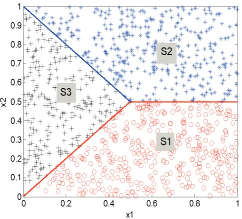
Clearly, , see Figure 1 for a clearer visualisation. One thousand data points

were generated from (22) by setting ] 1 , 0 [ ] 1 , 0 [ 3 2

1 S S = ×

S _{U U}

e x x f t

y( )= ( ₁, ₂)+ , where the two input variables and

were uniformly distributed in [0,1], and e was a Gaussian noise with zero mean and standard

derivation 0.1. The distribution of the 1000 input data points in the three subspaces and is

shown in Figure 1, and the first return map formed by the 1000 data points is shown in Figure 2. The

predictor vector (the ‘input’ vector) was chosen to be , and the initial polynomial

and wavelet model was respectively chosen to be

) ( 1 t u ) ( 2 t u 2 1,S

S S3

T t x t x

t) [ ( ), ( )]

( = _{1 2}

x

∑

∑ ∑

= = = + + + = = 2 1 2 2 1 0

1 2 1

2 1 2 1 1 1

1 () () ()

)) ( ( ˆ ) (

i i i ii i i i i i

t x t x t x t f t

y x θ θ θ

∑

∑

= =

+ 2 2 1 5 4

5 1 5 1 1 ) ( ) ( i

i i i i i i

t x t

x _L

L θ L

)) ( ( ˆ )

(t f t

y = x

∑ ∑ ∑

= ∈ ∈ ⎪⎭ ⎪ ⎬ ⎫ ⎪⎩ ⎪ ⎨ ⎧ = 4

0 1 2 ; , ; , 1 2 2

1 2

1 ( ( ), ())

j k Bjk Bjjk k jk k

t x t x

c ψ (24)

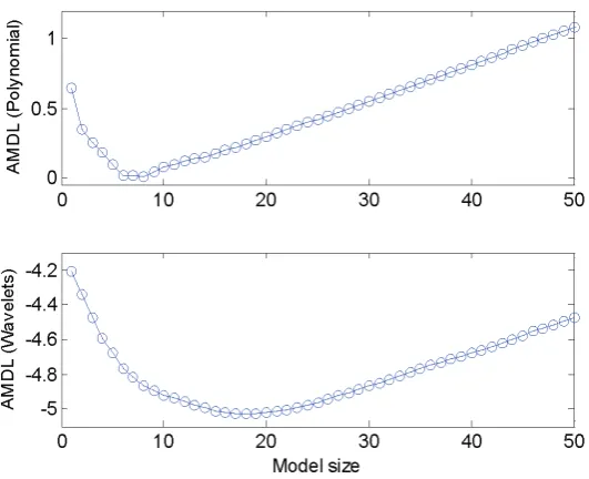
The total number of candidate model terms (basis functions) involved in the initial polynomial model (23) and the initial wavelet model (24) was 21 and 893, respectively. Based on the 1000 data points, the OLS-ERR algorithm was applied to select significant model terms for both the polynomial and the wavelet model identification. The AMDL criterion, shown in Figure 3, suggested that the number of model terms for the polynomial and wavelet models was 17 and 36 respectively.

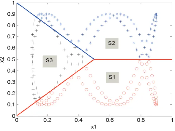
To inspect and compare the performance of the identified 17-term polynomial model and 36-term wavelet model, both models were simulated by choosing the two input variables and as

below:

) ( 1 t

u u2(t)

• Both and were uncorrelated random sequences, with 500 data points, uniformly

distributed in [0,1], but note that the test data was different from the data used for model estimation.

) ( 1 t

u u₂(t)

• u₁(t)=0.5+0.4sin(πt/50) andu₂(t)=0.5+0.4sin(πt/20+π/3) for t=1,2,…,500. The 500

input data points in the three subspaces S₁,S₂andS₃ is shown in Figure 4.

Model predicted outputs, from both the identified polynomial and wavelet models, were compared with that produced from the true noise-free model (22). The predicted results, corresponding to the above two test cases, are shown in Figures 5 and 6, respectively, where only a fraction of the data points is displayed for a closer visualisation. For the first test case, the mean-square-error (MSE), for the model predicted outputs from the identified polynomial and wavelet models, was calculated to be 0.2768 and 0.0923, respectively, over all the 500 test data points. For the second test case, the MSE was calculated to be 0.3719 and 0.1073, respectively, over the test data set. Clearly, the identified wavelet model is significantly superior to the polynomial model for the regime-switching system described by (22).

4.2 Example 2

A nonlinear system was described by the following model

⎪ ⎪ ⎩ ⎪⎪ ⎨ ⎧ < − − + − + − + − + − + − − ≥ − − + − + − + − + − − − − = , 0 ) 2 ( ) 1 ( if ), ( ) 1 ( )] 2 ( ) 1 ( [ 10 )] 2 ( 5 . 0 ) 1 ( )[ 2 ( , 0 ) 2 ( ) 1 ( if ), ( ) 1 ( )] 2 ( ) 1 ( [ 10 )] 2 ( 5 . 0 ) 1 ( )[ 1 ( ) ( 2 / 1 2 2 2 / 1 2 2 t x t x t t u t x t x t x t x t x t x t x t t u t x t x t x t x t x t x ξ ξ (25a) ) ( ) ( )

(t x t t

y = +η (25b)

whereξ(t)and )η(t were Gaussian white noise with zero mean and standard deviationσ_ξ=0.1 and

η

in [-10,10], model (25) was simulated and 500 input-output data points were collected after the system has settled down.

Figure 1. The three subspaces and , and the distribution of the 1000 input data points used for model estimation described in Example 1.

2 1,S

S S3

Figure 3. AMDL index versus the number of model terms for the polynomial models (the plot at the top) and the wavelet models (the plot at the bottom) identification described in Example 1.

Figure 5. A comparison of the model predicted outputs produced by the identified polynomial and wavelet models, with the true values produced by the noise-free model (22), driven by the input in the first test case described in Example 1. Circles present the true values, dots present the model predicted output from the wavelet model, and crosses present the model predicted output from the polynomial model.

The predictor vector was chosen to be . The

initial polynomial model was chosen to be

T t x t x t x

t) [ ( ), ( ), ( )]

( = _{1 2 3}

x _{=[y(t−1),y(t−2),u(t−1)]}T

∑

∑ ∑

= = = + + + = = 3 1 3 3 1 0

1 2 1

2 1 2 1 1 1

1 () ( ) ()

)) ( ( ˆ ) (

i i i ii i i i i i

t x t x t x t f t

y x θ θ θ

∑

∑

= =

+ 3 3 1 4 3

4 1 4 1 1 ) ( ) ( i

i i i i i i

t x t

x _L

L θ L

A total of 35 candidate model terms was involved in this polynomial model. The initial wavelet model was chosen to be

y(t)= fˆ(x(t))

_∑

_{∑ ∑}

p q pq p q p p p

t x t x f t x f

A total of 3012 candidate wavelet basis functions were involved in the initial wavelet model (27). Note that original observed data were initially normalized to [0,1], via the transform

) /( ) ) ( ~ ( )

( i i i i

i t x t a b a

x = − − , where ~xi(t) indicates the initial observations, and , for

i=1,2 (corresponding to the output variables), and

15

− =

i

a bi=15

10

− =

i

a ,bi=10for i=3 (corresponding to the input

variable). The identification procedure was performed using the normalized values of . The

outputs of an identified model were then recovered to the original measurement space by taking the associated inverse transform.

) (t xi

Based on the 500 estimation data points, the OLS-ERR algorithm was applied to select significant model terms for both the polynomial and the wavelet model identification. The AMDL criterion, shown in Figure 7, suggested that the number of model terms for the polynomial and wavelet models was 8 and 18 respectively.

To inspect and compare the performance of the identified 8-term polynomial model and the 18-term wavelet model, both models were simulated by choosing the input as a random sequence, with 500 data points, that was uniformly distributed in [-10,10]. Model predicted outputs, from both the polynomial and wavelet modes, were compared with that produced by the true model (25), and these are shown in Figure 8, where again only part data points were displayed. The MSE was calculated to be 0.7588 and 0.6870, respectively, with respect to the model predicted outputs from the identified polynomial and wavelet models, over the all 500 test data points. Clearly, the identified wavelet model is apparently superior to the polynomial model for the regime-switching system described by (25).

4.3 Example 3

A nonlinear system model was given by

⎜ ⎜ ⎜ ⎝ ⎛ ∈ − + − − − − ∈ − + − − − + ∈ − − − − − + − = 3 2 1 0 2 2 1 0 1 2 1 0 ), 1 ( ) 2 ( ) 1 ( ), 1 ( ) 2 ( ) 1 ( ), 1 ( ) 2 ( ) 1 ( ) ( S t u t x b t x b b S t u t x b t x b b S t u t x a t x a a t x ζ ζ ζ

, (28a)

) ( ) ( )

(t x t e t

Figure 7. AMDL index versus the number of model terms for polynomial model (the plot at the top) and wavelet model (the plot at the bottom) identification described in Example 2. The AMDL criterion for the wavelet model was calculated in the normalised space.

where

,

,

,

,

,

,

e

(

t

) was a noise signal,

, and the three subspaces

2 ( ), 1 (

[ − −

= x t x t

ζ S₁,S₂ S₃

} 25 . 0 : ) ,

{( 2

1 2

2 1

1 x x x x

S = ≥

,

,

,

1 2

2 1

2 = x x x < x x ≤

S {( , ): 0.25 2, ₁ 0}

1 2

2 1

3 = x x x < x x >

S

Clearly the union of and is the whole plane in the 2-D space. By setting e(t) to be Gaussian

white noise with zero mean and standard deviation 2

1,S

S S3

e

σ =5, and by choosing the input u(t) as a random

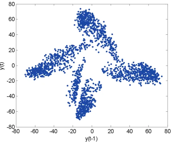
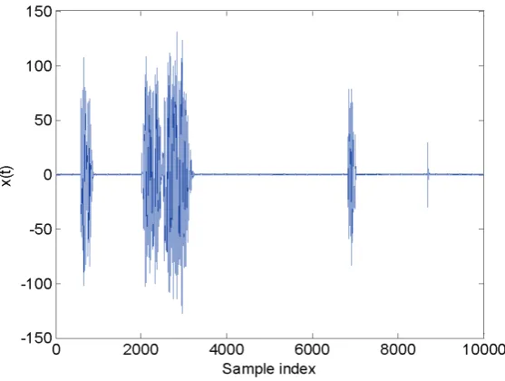
sequence that was uniformly distributed in [-5,5], model (28) was simulated and 2500 input-output data points were collected after the system has settled down. The first 500 data points was used for model estimation and the remaining 2000 data points were used for model validation. The first return maps produced by the 2000 noisy test data and the associated noisy-free data are shown in Figures 9 and 10, respectively.

Note that the output of the model (28a) was sensitive to the model parameters. For example, a small disturbance in the parameter may lead to a dramatic difference in the model response under

the same input. Figure 11 presents this phenomenon, where the difference 2

b

) ; ( ) ; ( )

(t = y t b2+δ −y t b2

ε ,

with =0.8 and , was displayed. Clearly, with the process going on, a small discrepancy in

the parameter produces significant difference in the model response. This means that it might be

difficult to identify a model that can produce accurate long term predictions. 2

b _{δ =10}−4

2

b

The predictor vector, the initial polynomial model, and the initial wavelet model were chosen exactly the same as in Example 2. The original observed data were initially normalized to [0,1], by settingai=−80andbi=80for i=1,2 (corresponding to the output), andai =−5and for i=3

(corresponding to the input). The identification procedure was performed using normalized values of

. The outputs of an identified model were then recovered to the original measurement space by

taking the associated inverse transform. Based on the 500 data points, the OLS-ERR algorithm was applied to select significant model terms for both the polynomial and the wavelet model identification. The AMDL criterion suggested that the number of model terms for the polynomial and wavelet models was 12 and 21 respectively.

5

− =

i b

) (t xi

map formed by the original measurements. This means that the identified wavelet model is superior to the associated polynomial model for the nonlinear regime-switching system described by (28).

Figure 9. The first return map formed by the 2000 noisy training data points generated by model (28) in Example 3.

-

Figure 10. The differenceε(t)=y(t;b₂+δ)−y(t;b₂)produced by the noise-free model (28a), described in Example 3, where_{δ =10}−4.

Figure 13. The first return map produced by the model predicted output of 2000 data points from the identified wavelet model, driven by a random sequence that was uniformly distributed in [-5,5].

5. Conclusions

A new wavelet based modelling approach has been introduced for nonlinear regime-switching system identification, where it was assumed that the inherent model structure and relative regime switches of the underlying systems are totally unknown. For this type of severely nonlinear systems, where a priori knowledge on the model structure is unavailable, identifying a global input-output model, from available data, may be a good initial step towards further understanding of the underlying dynamics. It has been demonstrated that wavelets, with local properties in both the time and the frequency domains, are powerful for constructing global nonlinear models for regime-switching systems. The performance of the resultant wavelet models, as has been shown, is much superior to that of the associated polynomial models for dealing with the identification problems described in the examples.

Wavelet bases, in dynamical wavelet modelling, involve two key parameters: the scales (the dilation parameter) and the positions (the translation parameter). While it is believed that the higher the scales the more accurate the wavelet model is, experience from numerous case studies has shown that the dilation parameter need not to be chosen very high. As a rule of thumb, setting the scale parameter to values up to 2 or 3 can often work well.

The selection of significant variables is a crucial step that could greatly improve the accuracy of all model construction procedures. Often, the ‘input’ vector of a model is formed by the selected significant variables. The number of significant variables is closely related to the model order that is determined by the maximum lags of the system input and output variables. In the present study, it was assumed that both the model order and the predictor vector of the model are known. If no apriori information on the predictor vector is available, some model order and variable selection algorithms need to be initially applied to determine an appropriate model order and the relevant primary model variables; the determined model variables can then be used to construct a nonlinear model.

Acknowledgements

The authors gratefully acknowledge that this work was supported by EPSRC (UK).

References

A. Antoniadis, I. Gijbels, G. Gregoire, “Model selection using wavelet decomposition and applications”, Biometrika, 84(4), pp. 751-763, 1997.

P. J. Antsaklis and A. Nerode, “Hybrid control systems: An introductory discussion to the special issue”, IEEE Trans. Automatic Control, 43(4), pp.457-460, 1998.

A. Bemporad, G. Ferrari-Trecate, and M. Morari, “Observability and Controllability of piecewise affine and hybrid systems”, IEEE Trans. Auto. Control, 45(10), pp. 1864-1876, 2000.

S. A. Billings and S. Chen, “The determination of multivariable nonlinear models for dynamic systems using neural networks”, In C.T. Leondes (Ed.), Neural Network Systems Techniques and

Applications, San Diego: Academic Press, pp. 231-278, 1998.

S. A. Billings, S. Chen, S., and M. J. Korenberg, “Identification of MIMO non-linear systems suing a forward regression orthogonal estimator”, Int. J. Control, 49(6), pp. 2157-2189, 1989.

S. A. Billings and W. S. F. Voon, “Piecewise linear identification of non-linear systems”, Int. J. Control, 46(1), pp.215-235, 1987.

S. A. Billings and H. L. Wei, “A new class of wavelet networks for nonlinear system identification”, IEEE Trans. Neural Networks, 16(4), pp. 862-874, 2005.

S. Chen and S. A. Billings, “Representations of non-linear systems - the NARMAX model”, Int. J. Control, 49(3), pp.1013-1032, 1989.

S. Chen, S. A. Billings, and W. Luo, “Orthogonal least squares methods and their application to non-linear system identification”, Int. J. Control, 50(5), pp.1873-1896, 1989.

V. Cherkassky and F. Mulier, Learning from Data, New York: John Wiley & Sons, 1998. J. H. Friedman, “Multivariate adaptive regression splines”, Ann. Stat., 19(1), pp. 1-67, 1991. J. D. Hamilton, “A new approach to the economic analysis of nonstationary time series and the

business cycle”, Econometrica, 57(2), pp.357-384, 1989.

J. D. Hamilton, Time Series Analysis, Princeton, N.J.: Princeton University Press, 1994.

C. J. Harris, X. Hong, and Q. Gan, Adaptive Modelling, Estimation and Fusion from Data: A Neurofuzzy Approach, Berlin: Springer-Verlag, 2002.

I. J. Leontaritis and S. A. Billings, “Input-output parametric models for non-linear systems—part 1: deterministic non-linear systems”, Int J. Control, 41(2), 303-328, 1985a.

I. J. Leontaritis and S. A. Billings, “Input-output parametric models for non-linear systems—part 2: Stochastic Non-Linear Systems”, Int J. Control, 41(2), 329-344, 1985b.

L. Ljung, System Identification : Theory for the User, Englewood Cliffs : Prentice-Hall, 1987.

G. Li, C. Rosenthal, and H. Rabitz, “High dimensional model representation”, J. Physical Chemistry, 105(33), pp. 7765-7777, 2001.

G. P. Liu, Nonlinear Identification and Control: A Neural Network Approach, Berlin: Springer-Verlag, 2001.

R. Murry-Smith and T. A. Johansen (ed.), Multiple model approaches to modelling and control, London : Taylor & Francis, 1997.

R. K. Pearson, Discrete-Time Dynamic Models, Oxford: Oxford University Press, 1999.

J. Rissanen, “A universal prior for integers and estimation by minimum description length”, Ann. Stat., 11, pp. 416-431, 1983.

N. Saito, “Simultaneous noise suppression and signal compression using a library of orthonormal bases and the minimum description length criterion”, In Wavelet in Geophysics, Foufoula-Georgiou, E. and Kumar, P., Eds, New York: Academic, pp. 299-324, 1994.

E. D. Sontag, “Nonlinear regulation: the piecewise linear approaches”, IEEE Trans. Auto. Control, 26(2), pp. 346-358, 1981.

T. Söderström and P. Stoica, System Identification, New York : Prentice Hall, 1989.

H. L. Wei and S. A. Billings, “A unified wavelet-based modelling framework for nonlinear system identification: the WANARX model structure”, Int. J. Control, 77(4), pp. 351-366, 2004.

H. L. Wei, S. A. Billings, and M. A. Balikhin, “Prediction of the Dst index using multiresolution wavelet models”, J. Geophys. Res, 109(A7), A07212, doi:10.1029/2003JA010332, 2004a.

H. L. Wei, S. A. Billings, and J. Liu, “Term and variable selection for nonlinear system identification”, Int. J. Control, 77(1), pp. 86-110, 2004b.