Data Augmentation in the Bayesian Multivariate Probit Model

This is a repository copy of Data Augmentation in the Bayesian Multivariate Probit Model.

White Rose Research Online URL for this paper:

http://eprints.whiterose.ac.uk/9887/

Monograph:

León-González, R. (2004) Data Augmentation in the Bayesian Multivariate Probit Model.

Working Paper. Department of Economics, University of Sheffield ISSN 1749-8368

Sheffield Economic Research Paper Series 2004001

Reuse

Unless indicated otherwise, fulltext items are protected by copyright with all rights reserved. The copyright exception in section 29 of the Copyright, Designs and Patents Act 1988 allows the making of a single copy solely for the purpose of non-commercial research or private study within the limits of fair dealing. The publisher or other rights-holder may allow further reproduction and re-use of this version - refer to the White Rose Research Online record for this item. Where records identify the publisher as the copyright holder, users can verify any specific terms of use on the publisher’s website.

Takedown

If you consider content in White Rose Research Online to be in breach of UK law, please notify us by

Sheffield Economic Research Paper Series

SERP Number:

2004001

Roberto León González

Data Augmentation in the Bayesian Multivariate Probit Model

January 2004

Department of Economics University of Sheffield 9 Mappin Street Sheffield S1 4DT

United Kingdom

Data Augmentation in the Bayesian Multivariate Probit

Model

∗

Roberto Le´

on Gonz´

alez

Department of Economics

University of Sheffield

January 2004

Abstract

This paper is concerned with the Bayesian estimation of a Multivariate Probit

model. In particular, this paper provides an algorithm that obtains draws with low

correlation much faster than a pure Gibbs sampling algorithm. The algorithm consists

in sampling some characteristics of slope and variance parameters marginally on the

latent data. Estimations with simulated datasets illustrate that the proposed algorithm

can be much faster than a pure Gibbs sampling algorithm. For some datasets, the

algorithm is also much faster than the efficient algorithm proposed by Liu and Wu

(1999) in the context of the univariate Probit model.

∗_{This paper was circulated before as part of the discussion paper 09/02 of the Department of Economics}

1

Introduction.

Data augmentation (Tanner and Wong, 1988) was an important development in the

field of Markov Chain Monte Carlo algorithms. When it is combined with the pioneer

works of Metropolis et al. (1953) and Hastings (1970) it makes the Bayesian analysis

of more complex models possible. Data augmentation consists in regarding latent

and missing data as parameters to estimate. Although this introduces many more

parameters, the conditional densities became much easier to sample from.

Although data augmentation facilitates the design of an algorithm, convergence

might be slow due to high correlation between model parameters and latent data.

Large autocorrelations imply that the chain moves slowly along the parameter space.

Slow movement causes three types of problem. Firstly, a large number of iterations

is needed for the chain to converge. In addition, a large number of iterations will be

needed to obtain a representative sample of the posterior density. Furthermore, an

even larger number of iterations are needed to be able to determine whether the chain

has converged. A representative sample from the posterior density can be obtained

after the chain has traveled along the parameter space just once. However, evidence

of convergence requires that the chain has recovered the same region repeatedly. For

these reasons it is advised (e.g. Raftery and Lewis 1992, Gilks and Roberts 1995) that

when a chain is very slow an alternative algorithm must be designed.

The aim of this paper is to provide new tools to reduce the autocorrelations of the

chain and hence enhance the reliability of the calculations in the Bayesian Multivariate

Probit model. These strategies can potentially be applied to a wider range of Bayesian

models.

The algorithm proposed in this paper combines both the Gibbs sampling and the

Metropolis algorithm. Although data augmentation is used, some characteristics of

slope and variance parameters are updated marginally on the latent data. These

characteristics are sampled using a re-parameterisation of the posterior density.

Estimation with a simulated dataset shows that the proposed algorithm can produce

draws with low correlation much faster than a pure Gibbs sampling algorithm. In the

with the PX-DA algorithm designed by Liu and Wu (1999). It is shown that the

proposed algorithm substantially outperforms the PX-DA algorithm for some datasets.

The plan of the paper is as follows. Section 2 describes the Multivariate Probit

model and the prior density. Section 3.1 and 3.2 outline the proposed algorithm for

the Univariate and Multivariate Probit model, respectively. Section 4 uses simulated

data to illustrate the performance of the proposed algorithm in comparison with a pure

Gibbs sampling algorithm (Leon-Gonzalez, 2003) and the PX-DA algorithm (Liu and

Wu, 1999). Section 5 draws some conclusions.

2

The Multivariate Probit Model

The Multivariate Probit model can be described as follows. LetYi be a vector of zeros

and ones. Each componentyit of Yi is determined by a continuous unobserved latent

variabley∗

it generated according to the following process,

y∗

it=Xitβt+eit i= 1, ..., N t= 1, ..., T (1)

the vector ei = (ei1, ..., eiT)T is normally distributed with zero mean and covariance

matrix Σ = (σjk). The binary variable yit is equal to one if and only ifyit∗ ≥ 0, and

is equal to zero otherwise. Xit is a 1×kt vector of regressors and βt is a vector of

parameters.

The most common normalisation in the literature (e.g. Chib and Greenberg, 1998)

is to fix:

σ11=σ22=...=σT T = 1 (2)

However, with this normalisation Σ cannot be sampled directly from its conditional

density, and a Metropolis step is necessary (Chib and Greenberg, 1998). It is possible

to avoid this by following the normalisation restriction and the prior density proposed

by Leon-Gonzalez (2003). In this way, it is possible to sample Σ directly from its

conditional posterior, and hence it is possible to use a pure Gibbs sampling algorithm.

Thus, we use the following normalisation:

where σT T·12...(T−1) =V ar

³

eiT|ei(T−1), ..., ei1

´ .

Let the prior for Σ be an Inverted Wishart IWT (df0, K0) distribution conditional

to restriction (3). That is, the kernel of the prior for a matrix Σ that verifies restriction

(3) is:

|Σ|−df0/2

exp³−1/2tr³Σ−1_K 0

´´

(4)

It can be shown that normalisation (3) is equivalent to fixing the diagonal elements

of the Cholesky decomposition of Σ equal to 1 (Leon-Gonzalez, 2003). Hence,

normalisation (3) guarantees that the matrix Σ is positive definite. Hence, no further

restriction holds on the parameters in Σ.

Let us assume that the vector of slope parameters nβ₁T, β₂T, ..., β_TToT is a priori

independent of Σ and follows a normal density with meanβ0 and variance-covariance

matrixV0.

The conditional posterior of Σ given parameters β and latent data {y∗

it : t = 1, ... , T}T_i=1 is an inverted Wishart IWT (df, K) conditional to restriction (3). The

parameters of this inverted Wishart are df = df0 +N and K = K0 +PNi=1eieTi .

A draw from this density can be obtained with a simple algorithm (Leon-Gonzalez

2003).

Note that the MCMC sample from the posterior density under normalisation (3)

can be transformed to obtain a sample from the posterior of the parameters under

normalisation (2) (Leon-Gonzalez, 2003). Hence, the use of normalisation (3) in the

calculations does not preclude us from obtaining estimates according to restriction (2).

3

Data

Augmentation

in

the

Multivariate

Probit Model.

For simplicity in the exposition, we first focus in the case of the probit model, that is

3.1

The Univariate Probit.

The algorithm proposed in this section results from adding one step to the Gibbs

sampling algorithm. The additional step proposes a move of model parameters that is

carried out without conditioning on the latent data. In particular, slope parameters

are multiplied by a random factor, and this random factor is sampled marginally on

the latent data. The random factor is one variable from a re-parameterisation of the

model.

Assuming that there are k1 explanatory variables in the equation, let β1 =

(β11, ..., β1k1)

T_{, and consider the following re-parameterisation of the model,}

β1 =

µ β11,

β12

β11

,β13 β11

, ...,β1k1 β11

¶

=³β11, β12, ..., β1k1

´

y∗

i1 = Xi11β11+Xi12β12β11+Xi13β13β11+...+Xi1k1β1k1β11+ei1

The posterior distribution of β1, denoted by πM(.), is derived from the posterior

density ofβ1 (πM) in this way:

πM ³

β11, β12, ..., β1k1|Y1, ..., YN

´ =πM

³

β11, β12β11, ..., β1k1β11|Y1, ..., YN

´

|β11|k1−1

where¯¯_¯βk1−1

11

¯ ¯

¯ is the Jacobian of the transformation. The proposed algorithm is:

Algorithm 1

Step 1: Sample ³β11, β12, ..., β1k1

´

conditional on (Y∗

1, ..., YN∗)

Step 2: Sample β11 conditional on

³

β12, ..., β1k1

´

Step 3: Sample (Y∗

1, ..., YN∗) conditional on ³

β11, β12, ..., β1k1

´

Note that Algorithm 1 is the same as a Gibbs algorithm, with an additional step

2. Hence, it is just a Gibbs sampling algorithm in which all slope parameters (of the

original parameterisation) might be multiplied by a random factor. Whenever a new

value is drawn in the second step, all slope parameters move in the same direction.

Step 2 accelerates the algorithm because it proposes a change of all parameters that is

unconditional on the latent data. Conditioning on latent data makes the parameters

move substantially more slowly.

The conditional distribution of (Y∗

1, ..., YN∗) is the same as in the algorithm proposed by Chib and Greenberg (1998). The vector ³β11, β12, ..., β1k1

´

generating (β11, β12, ..., β1k1) conditional on (Y1∗, ..., Y_N∗) and then transforming the

variables in this way: ³β11, β12, ..., β1k1

´

= (β11, β12/β11, ..., β1k1/β11).

The conditional distribution of β11 given

³

β12, ..., β1k1

´

does not have a standard

form. Hence, a metropolis step can be used to generateβ11. The proposal density for

the Metropolis step could be a normal with mean and variance equal to the Maximum

Likelihood estimation ofβ11. Alternatively,β11 can be generated with a random walk.

Step 2 can be repeated a number of times to increase the probability of accepting a

new value. A more detailed description of the algorithm can be found in the Appendix.

3.2

The Multivariate Case

The algorithm for the multivariate case proposed in this section adds T steps to the

Gibbs sampling algorithm. Each of these steps proposes to move slope and

variance-covariance parameters for one equation jointly and without conditioning on the latent

data for the corresponding equation. This move consists in multiplying the parameters

by a random factor. This random factor is a variable from a re-parameterisation of the

model and it is sampled marginally on the latent data.

Consider the following parameterisation of the multivariate probit model.

y∗

it=Xit1βt1+Xit2βt2βt1+Xit3βt3βt1+...+Xitktβtktβt1+eit t= 1, ..., T (5)

where:

βt = µ

βt1,

βt2

βt1

,βt3 βt1

, ...,βtkt

βt1

¶

=³βt1, βt2, ..., βtkt

´

t= 1, ..., T

Σ2 = (σ12/(β11β21), σ13/(β11β31), ..., σ1T/(β11βT1)) = (σ12, σ13, ..., σ1T)

Σ3 = σ23/(β21β31), σ24/(β21β41), ..., σ2T/(β21βT1) = (σ23, σ24, ..., σ2T)

...

ΣT = σ(T−1)T/ ³

βT1β(T−1)1

´

=σ_(T−1)T

With this parameterisation, the covariance matrix of (ei) is equal to:

Σ =         

σ11 σ12β11β21 ... σ1Tβ11βT1

σ12β11β21 σ22 ... σ2Tβ21βT1

...

where (σ11, σ22, ..., σT T) are determined by normalization (3) (e.g. σ22 = 1 +

(σ12β11β21)2).

Let {(βt)n:t= 1, ..., T}, (Σ)n be the nth value of {βt:t= 1, ..., T}, Σ in the

proposed MCMC chain. The following algorithm describes how to obtain this value.

Algorithm 2.

Step 1: Sample ³β1, β2, ..., βT ´

conditional on (Y∗

1, ..., YN∗,Σ).

Step 2: Sample nΣt:t= 2, ..., T o

conditional on ³β1, β2, ..., βT, Y1∗, ..., YN∗ ´

Step 3: For t= 1, ..., T do:

• Generate βt1 conditional on {y∗_ik:k6=t}i=1,...,N,

n

βtk :k6= 1 o

, nβj :j6=t o

,

n

Σt:t= 2, ..., T o

.

• Sample {y∗

it}i=1,...,N conditional on the most recent values of ³

β1, β2, ..., βT ´

,

n

Σt:t= 2, ..., T o

and {y∗

ik :k6=t} i=1,...,N

Step 4: Fix

(βt)n = (βt1, βt1βt2, ..., βt1βtkt) f or t= 1, ..., T

(Σ)n =         

σ11 σ12β11β21 ... σ1Tβ11βT1

σ12β11β21 σ22 ... σ2Tβ21βT1

...

σ1Tβ11βT1 σ2Tβ21βT1 ... σT T         

where (σ11, σ22, ..., σT T) are determined by normalization (3)

The first part of Step 3 uses a Metropolis step to update the slope parameters

and covariance terms (of the original parameterisation) jointly and marginally on the

latent data. It can be repeated several times to increase the likelihood of acceptance

of a new value. In the simulations of Section 4, the proposal density in the Metropolis

step is a random walk. Alternatively, it is possible to specify a normal density centered

on Maximum Likelihood estimates. These Maximum Likelihood estimates could be

obtained before the MCMC chain is started from separate estimation of the T equations

using univariate Probit models.

Step 1 is carried out by sampling first (β1, β2, ..., βT) as explained in Chib and

Greenberg (1998) and transforming the values to obtain³β1, β2, ..., βT ´

Step 2 is carried out by sampling first Σ and transforming the values to obtain n

Σt:t= 2, ..., T o

. The density of Σ is an inverted Wishart subject to restriction (3).

This density can be sampled directly (Leon-Gonzalez 2003).

The latent data in the second part of Step 3 are sampled as described by Chib and

Greenberg (1998): from truncated normals and according to equations (5) and (6).

4

Comparing

the

Performance

of

the

Algorithms.

4.1

Univariate Probit Model.

This section compares Algorithm 1 with a standard Gibbs Sampling algorithm and

the PX-DA algorithm (Liu and Wu, 1999). Algorithm 1 is implemented with step 2’

repeated 4 times. 8400 observations for seven explanatory variables were generated

independently from a standard normal distribution. Slope coefficients are:

β11= 1, β12= 2, β13= 0.5, β14=−0.2, β15=−1, β16= 0.8, β17= 0.8

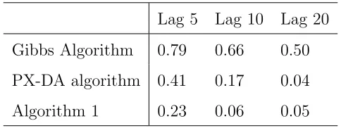
Table 4.1 shows the value of the highest correlation for lags 5, 10 and 20.

Auto-correlations in the chain are calculated using 29000 iterations after discarding the

first 1000 iterations. The initial value of parameters was equal to zero.

Auto-correlations in Algorithm 1 are the lowest, being less than half the autoAuto-correlations

in the PX-DA algorithm. In the Gibbs sampling algorithm, 80 lags are necessary

for the autocorrelations of all parameters to be below 0.1. The PX-DA algorithm

achieves the same with 20 lags. Algorithm 1 needs the lowest amount of lags, 10, for

all correlations to be below 0.1.

The highest correlation for all algorithms, except for Algorithm 1, correspond to

β12. As noted by Liu and Wu (1999), autocorrelations in the probit model increase

with the absolute value of the coefficients. In contrast, the autocorrelation of β12 in

Algorithm 1 is the lowest, and the highest correspond to parameter β14, that has the

Lag 5 Lag 10 Lag 20

Gibbs Algorithm 0.79 0.66 0.50

PX-DA algorithm 0.41 0.17 0.04

Algorithm 1 0.23 0.06 0.05

Table 1: Maximum Autocorrelation of the Parameters

Large auto-correlations make it more difficult to determine whether the chain has

converged. With 29000 Gibbs sampling iterations, after discarding the first 1000

iterations, the Geweke test (1992) rejects the null hypothesis of convergence for 3

out of 7 parameters. With the same number of iterations, the test accepts the null

hypothesis of convergence of all the parameters in the other two algorithms.

The Gibbs algorithm and the PX-DA algorithm have similar computation

time. However, Algorithm 1 needs approximately double computing time with this

implementation. Taking this into account, Algorithm 1 produces 2 draws with

correlation smaller than 0.1 four times faster than a Gibbs Sampling algorithm.

However, there is almost no advantage over the PX-DA algorithm, since similar

values for correlations can be obtained with approximately the same computing time.

However, as the following example shows, when slope parameters have a larger value

the gains in autocorrelation clearly outweigh the losses in computation time.

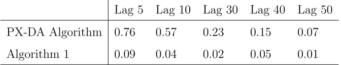
A similar exercise is carried out, with the same number of observations, but letting

the value of the parameters be:

β11= 3, β12= 3, β13= 3, β14=−3, β15=−3, β16=−3, β17= 3

Table 2 shows the maximum autocorrelation of the parameters. The PX-DA

algorithm needs at least 50 lags for all autocorrelations to be below 0.1. Algorithm

1 has all autocorrelations below 0.1 with just 5 lags. Hence, the substantial gains

in smaller autocorrelations in Algorithm 1 more than compensate for the additional

computation time per iteration. That is, with this dataset Algorithm 1 obtains two

Lag 5 Lag 10 Lag 30 Lag 40 Lag 50

PX-DA Algorithm 0.76 0.57 0.23 0.15 0.07

Algorithm 1 0.09 0.04 0.02 0.05 0.01

Table 2: Auto-correlations when parameters have a large value

4.2

Multivariate Probit Model.

This section compares the performance of Algorithm 2 with a standard Gibbs

algorithm. Two versions of Algorithm 2 are implemented: in one the first part of

step 3 is repeated 3 times (Algorithm 2a), and in the other it is carried out just once

(Algorithm 2b).

The data was generated according to the following random-effects type process:

y∗

it = 1∗x1i+ 2∗x2i+ 0.5∗x3i−0.2∗x4i−1∗x5i+ 0.8∗x6i +0.8∗x7i+ui+eit

i = 1, ...,1200 t= 1, ...,7

where (ei1, ..., eiT) follows aN(0, I),ui follows a N(0,1), and it is independent ofeit.

The regressors are invariant witht and are generated independently from a standard

normal distribution. The prior for the slope parameters is a normal distribution with

zero mean and covariance matrix equal to 10000I. The prior for the free parameters in

Σ is a restricted inverted Wishart withK0 =I and df0 = 2∗T+ 1 = 15.

Hence, in this specification, 49 slope parameters plus 21 covariance parameters are

estimated. For simplicity, only the autocorrelations of the 7 slope parameters in the first

equation and 7 covariance parameters are analysed. Autocorrelations are calculated

with 9000 iterations after discarding the first 1000.

Table 3 shows that autocorrelations for slope parameters vanishes more quickly in

Algorithm 2. From Table 4, the Gibbs sampling algorithm has at least one covariance

parameter with a correlation as high as 0.13 after 100 lags. In fact, the Gibbs algorithm

needed 120 lags for the maximum autocorrelation to be below 0.1. In contrast, in

Algorithms 2a and 2b the maximum correlation for covariance parameters vanishes

The computing time per iteration in Algorithm 2a and 2b is 2.6 and 1.9 times

larger than in the Gibbs algorithm, respectively. The gains in lower autocorrelations

more than compensate for the extra computing time, since the number of iterations

needed for the Gibbs autocorrelations to be below 0.1 is about 4 and 3 times the

number of iterations needed in Algorithm 2a and 2b, respectively. In addition, unlike

the Gibbs Sampling algorithm, the chains produced by Algorithm 2a and 2b passed

the convergence test proposed by Heidelberg et al. (1983), hence further increasing the

reliability of the calculations.

Lag 10 Lag 20 Lag 30 Lag 40 Lag 50 Lag 100

Gibbs Algorithm 0.54 0.40 0.34 0.29 0.23 0.13

Algorithm 2a 0.29 0.13 0.08 0.04 0.04 0.007

Algorithm 2b 0.44 0.23 0.12 0.08 0.06 0.004

Table 3: Autocorrelations for covariance parameters

5

Conclusions

The motivation underlying the algorithms proposed in this paper is that a pure

Gibbs sampling algorithm moves slowly due to sampling separately variables that are

highly correlated. For this reason, the algorithms in this paper propose to sample

characteristics of model parameters not conditioning on the latent data. This is

Lag 10 Lag 20 Lag 30 Lag 40 Lag 50

Gibbs Algorithm 0.57 0.37 0.28 0.20 0.13

Algorithm 2a 0.33 0.17 0.09 0.06 0.04

Algorithm 2b 0.43 0.24 0.15 0.09 0.04

achieved by sampling from a re-parameterisation of the model. In this way, parameters

in the original parameterisation are updated marginally on the latent data.

Using simulated data, the previous section shows that Algorithm 2 can produce

two draws with low correlation faster than a pure Gibbs sampling algorithm. In the

simpler case of the univariate Probit model, the proposed Algorithm 1 was compared

with the efficient algorithm proposed by Liu and Wu (1999). It was shown that for

some datasets Algorithm 1 is substantially much faster.

The type of re-parameterisations considered in this paper facilitates the updating

of large numbers of parameters jointly and marginally on the latent data. This is

potentially applicable to many models with complex likelihoods, where conventional

Appendix

Let ³βn

11, β12n, ..., βn1k1

´

denote the nth _{value of (β}

11, β12, ..., β1k1) in the chain. If a random walk is used, the algorithm to generate the (n+1)th value of (β11, β12, ..., β1k1)

is:

Algorithm 1

Step 1. Sample (β11, β12, ..., β1k1) from a N(µp, Vp), where µp =

Vp³PNi=1XiT1Yi∗+V0−1β0

´

, and Vp=³PNi=1XiT1Xi1+V0−1

´−1

.

Step 2. Fix ³β12, ..., β1k1

´

= (β12/β11, ..., β1k1/β11). Generate a random scalar v

from a distribution with density function f(v). Fix

β₁₁n+1 =vβ11, β12n+1 =vβ11β12, ..., β₁n_k+11 =vβ11β1k1

with probability

γ = min

½_L(Y|vβ

11, vβ12, ..., vβ1k1)π(vβ11, vβ12, ..., vβ1k1) L(Y|β11, β12, ..., β1k1)π(β11, β12, ..., β1k1)

f(1/v) f(v)

¯ ¯ ¯vk1¯¯

¯,1 ¾

and fix

βn₁₁+1 =β11, β12n+1=β11β12, ..., β1nk+11 =β11β1k1

with probability (1−γ), where L(Y|β11, β12, ..., β1k1) is the likelihood function:

L(Y|β1) =

N Y

i=1

³

Φ (−Xi1β1)1−Yi(1−Φ (−Xi1β1))Yi

´

and π(β11, β12, ..., β1k1) is the prior density.

Step 3. Sample Y∗

i from a truncated

N³Xi11β11n+1+Xi12βn12+1+...+Xi1k1β

n+1 1k1 ,1

´

for all i= 1, ..., N.

Step 2 of the algorithm can be repeated a number of times to increase the likelihood

of acceptance of a new value.

The functionf(v) might be centred at 1, so that new candidates are drawn from a

to positive values, hence forcing new candidates to have the same sign as the previous

value. An inverted gamma would play this role.

Alternatively, the Metropolis step could use a normal density calibrated with the

Maximum Likelihood estimates of β11. If φN ³

x;βd11,sdd1

´

is the density function of

a N³dβ11,sdd1

´

centered at the maximum likelihood estimates, then Step 2 can be

implemented as:

• Step 2’. Fix ³β12, ..., β1k1

´

= (β12/β11, ..., β1k1/β11). Generate a random scalar

v from a distribution with density function φN ³

v;dβ11,sdd1

´

. Fix

β₁₁n+1=v, βn₁₂+1 =vβ12, ..., βn1k+11 =vβ1k1

with probability

γ′ _{= min}

  1,

L³Y|v, vβ12, ..., vβ1k1

´

π³v, vβ12, ..., vβ1k1

´

L(Y|β11, β12, ..., β1k1)π(β11, β12, ..., β1k1) φN

³ βn

11;βd11,sdd1

´

φN ³

v;βd11,sdd1

´ × ¯ ¯ ¯ ¯ ¯ µ _v β11

¶k1₋1¯¯

¯ ¯ ¯ )

and fix

β₁₁n+1 =β11, βn12+1 =β11β12, ..., β₁n_k+11 =β11β1k1

References

Chib., S. and Greenberg, E. (1998) ”Analysis of Multivariate Probit Models,”

Biometrika 85, 347-361.

Geweke, J., (1992) ”Evaluating the Accuracy of Sampling-Based Approaches to the

Calculation of Posterior Moments,” inBayesian Statistics, 4 (ed. J. M. Bernardo,

J. Berger, A. P. Dawid, and A. F. M. Smith) Oxford University Press, Oxford,

169-193.

Gilks, W. R., and Roberts, G. O. (1995) ”Strategies for improving MCMC,” In

Markov Chain Monte Carlo in Practice, (ed. W.R. Gilks, S. Richardson and

D.j. Spiegelhalter) Oxford University Press, Oxford, 89-114.

Hastings, W. K., (1970) ”Monte Carlo sampling methods using Markov chains and

their applications,”Biometrika, 57, 97-109.

Heidelberg, P., and Welch, P. D. (1983) ”Simulation Run Length Control in the

Presence of and Initial Transient,”Operations Research, 31, 1109-1144.

Leon-Gonzalez, R. (2003) ”Sampling the Variance-Covariance Matrix in the Bayesian

Multivariate Probit Model,” Discussion Paper SERP2003008, Department of

Economics, University of Sheffield

Liu, J. S., and Wu, Y. N., (1999) ”Parameter Expansion for Data Augmentation,”

Journal of the American Statistical Association, 94, 448, 1264-1274.

Metropolis, N., Rosenbluth, A. W., Rosenbluth, M. N., Teller, A. H. and Teller, E.

(1953) ”Equation of state calculations by fast computing machine,” Journal of

Chemical Physics 21, 1087-91.

Raftery, A. L. and Lewis, S. (1992) ”How many iterations in the Gibbs sampler?,” In

Bayesian Statistics 4, (ed. J. M. Bernardo, J. O. Berger, A. P. Dawid, and A. F.

M. Smith), 763-74. Oxford University Press, Oxford.

Tanner, T. A., and Wong, W. H. (1988) ”The Calculation of Posterior Distributions

by Data Augmentation,”Journal of the American Statistical Association 82,