Oxide Structure Prediction and
Synthesis
Thesis submitted in accordance with the requirements of the
University of Liverpool for the degree of Doctor in
Philosophy by:
Christopher Michael Collins
Supervised by
Professor M. J. Rosseinsky
Abstract
Abstract
Introduction: The focus of this chapter is to introduce the perovskite structure, beginning from the ideal cubit perovskite with the ABX3 formula unit. The concept of introducing long range ordering into the material are then presented along with the driving forces behind the extension of the structure. Possible magnetic ordering and solid solutions of perovskites are then presented. This is followed by the introduction of how theoretical chemistry can provide useful information to investigations and begin to predict how new materials can be made and is followed by a summary of the techniques commonly used.
Methods: This chapter introduces the experimental methods used within this thesis, along with a
description of the diffraction techniques used in the characterisation of oxide materials; including x-ray and neutron diffraction, iodometric titrations and the basic concepts behind Mössbauer spectroscopy. The second part to the chapter provides details on density functional theory (DFT) and force field (FF) calculations that are used throughout the thesis for the prediction of new materials.
Chapter 3: Details the use of a series of calculations with DFT on the chemical substitution in
the YBa2Fe3-xMxO8 (where M = Co, Ni and Mn), where the calculations are first tested on doping with Co, where it has been previously been experimentally reported. Calculations for un-reported substitutions a new compound is predicted. Synthetic investigations are then undertaken across the series, and a new material found where DFT calculations predict a new compound. Characterisation of the new material reveals that it has a crystal structure in good agreement with the structure predicted by DFT.
Chapter 4: Computationally investigates doping in the YBa2Ca2Fe5-xMxO13 (M = Co, Cu, Mn, Ni, Ti and Zn) solid oxide fuel cell cathode material using DFT. The results from the calculations predict stable doping for Cu and Co, with small doping levels favoured for M = Ni and Zn, with M = Mn yielding results predicting marginal doping and doping not favoured at all for M = Ti.
Chapter 5: When D. Hodgeman was experimentally investigating Cu doping of the
Acknowledgements
Acknowledgements
First and foremost I would like to thank my supervisors Prof. Matt Rosseinsky and Dr. George Darling, for all their guidance (and patience!) during the last four years along with their constant encouragement to learn new methods and techniques. I would also like to thank the rest of the research group with whom I have worked, notably Dr. Matthew Dyer for his never-ending patience with teaching me to use density functional theory, Dr. Antoine Demont and Dr. Phil Chater for their help with tutoring me in my synthetic chemistry and materials analysis and Dr. John Claridge for his seemingly infinite wisdom! I would also like to thank Dr. George Darling for getting computer time on the HECToR super computer through the Materials Chemistry Consortium (MCC), time which contributed enormously to the success of the calculations presented within chapters 4 and 5 of this thesis.
I would like to thank everyone around the surface science research centre and the MJR research group for making the time I have spent doing my PhD an enjoyable experience, especially all of those that have made cake over the years, even the ‘experimental’ cake – Olive oil and cake do not mix! and the ‘rock’ muffins!.
Outside of the workplace, I need to thank all of my friends and family for their kind support without whom I would not have made it through with any sanity remaining, along with their perseverance in telling me “It’ll all be ok”. Last but not least, a special mention has to go to Fiona for putting up with me all of these years, introducing me to radio comedy and finally taking the time to proof read this thesis, oh and cake, defiantly cake! I’ll leave it here with arguably the most common phrase used in my general direction during my PhD:
Contents
Contents
Chapter 1. Introduction ... 2
1.1 Concerning Perovskites ... 2
1.1.1 Cubic Perovskites... 2
1.1.2 Extended Perovskites ... 3
1.1.3 Magnetic ordering ... 10
1.1.4 Phase Diagrams and solid solutions ... 16
1.1.5 Doping perovskites and applications thereof ... 18
1.2 Theoretical calculations and solid state chemistry ... 20
1.3 Applications of theory to solid state chemistry ... 24
1.3.1 Formation/Reaction energies and material doping ... 24
1.3.2 Convex hulls52 ... 25
1.3.3 Data mining ... 28
1.3.4 Molecular dynamics and simulated annealing ... 30
1.3.5 Monte-Carlo ... 31
1.3.6 Site disorder ... 32
1.3.7 Genetic Algorithms ... 36
1.3.8 Secondary building units ... 38
1.4 Summary ... 40
1.5 Aims of this thesis... 42
Chapter 2. Synthetic and theoretical methods... 44
2.1 Solid state synthesis... 44
2.2 Diffraction from crystalline solids78 ... 46
2.3 Powder Diffraction81 ... 49
2.4 Laboratory based Powder X-ray Diffraction (PXRD)78... 51
2.5 Neutron Powder Diffraction (NPD)78, 81 ... 54
2.6 NPD at the ISIS neutron source on the High Resolution Powder Diffractometer (HRPD)89, 90 ... 55
2.7 Structure refinement78, 81 ... 57
2.7.1 Background, zero shift and peak shape... 59
2.7.2 Unit cell size and shape... 60
Contents
2.8 Iodometric titrations94 ... 63
2.9 Mössbauer Spectroscopy95 ... 67
2.10 Density Functional Theory18, 98 (DFT) ... 70
2.10.1 The energy functional ... 71
2.10.2 Exchange Correlation (XC) Functionals18, 101 ... 75
2.10.3 Plane wave solutions to the Kohn Sham equations18, 101, 104 ... 76
2.10.4 Pseudopotentials98 ... 78
2.10.5 DFT + U98 ... 80
2.11 Force Field (FF) Calculations69, 70... 81
2.11.1 Interatomic potentials... 82
2.11.2 Generating FF potential parameters ... 84
2.12 A note on computational hardware used. ... 85
Chapter 3. Prediction and synthesis of YBa2Fe2MnO8 ... 87
3.1 Abstract ... 87
3.2 Introduction ... 88
3.3 Computational methods ... 91
3.4 Experimental methods ... 96
3.5 Computational results ... 99
3.5.1 Results for M = Co ... 100
3.5.2 Results for M = Mn ... 103
3.5.3 Results for M = Ni ... 106
3.6 Experimental results ... 108
3.7 Discussion... 114
3.8 Conclusions ... 125
3.9 Tables ... 126
3.10 Appendix ... 130
Chapter 4. Doping predictions for YBa2Ca2Fe5-xMxO13 ... 136
4.1 Abstract ... 136
4.2 Introduction ... 137
4.3 Computational Setup ... 141
4.4 Results ... 149
Contents
4.4.2 Results for M = Co ... 153
4.4.3 Results for M = Cu ... 156
4.4.4 Results for M = Mn ... 162
4.4.5 Results for M = Ni ... 165
4.4.6 Results for M = Ti ... 168
4.4.7 Results for M = Zn ... 170
4.5 General Discussion ... 173
4.6 A Note on Subsequent Experimental Work Within The Research Group ... 176
4.7 Conclusions ... 177
4.8 Acknowledgements ... 177
4.9 Tables ... 178
Chapter 5. Extended Module Materials Assembly (EMMA) ... 184
5.1 Abstract ... 184
5.2 Introduction ... 185
5.3 Computational setup ... 189
5.4 Validating the EMMA method by finding the 10ap structure. ... 194
5.5 Using EMMA predict a structure for the 8ap. ... 197
5.6 Using EMMA to identify the 16ap structure ... 203
5.7 Discussion of results and comparison with experiment ... 205
5.7.1 Disorder matters ... 209
5.8 Discussion... 214
5.9 Conclusions ... 216
5.10 Tables ... 217
Chapter 6. Conclusions ... 221
Chapter 1. Introduction
Chapter 1.
Introduction
1.1
Concerning Perovskites
1.1.1 Cubic Perovskites
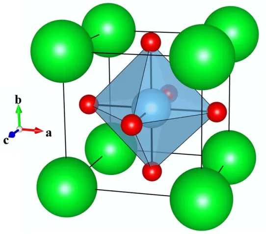
Figure 1 Structure of the cubic ABX3 perovskite, with this example being for SrTiO31, the A-site occupied by Sr (green) is coordinated to 12 oxygen atoms, the B-site is occupied by Ti (blue) and is in a 6 coordinate octahedral site and the unit cell also contains 3 oxygen atoms (red). In this thesis, to aid illustration of structures, polyhedra are drawn around each of the B-site cations with their coordination to oxygen anions.
[image:12.612.173.444.201.439.2]Chapter 1. Introduction
located at (0.5, 0.5, 0.5) and occupies a six coordinate octahedral site, the third is site occupied by the anion species at (0.5, 0.5, 0), with this site having a multiplicity of three. With a typical lattice parameter for a cubic perovskite, referred to as ap in the example of SrTiO3, ap is equal to 3.907 Å1.
1.1.2 Extended Perovskites
Figure 2 Orthorhombic crystal structure of CaTiO33 where Ca (blue) occupies the 12 coordinate A-site, Ti (cyan) occupies the octahedral six coordinate site, with oxygens illustrated in red.
[image:13.612.177.436.269.564.2]Chapter 1. Introduction
B O
OA r r r
r 2 (1.1)
Where indicates the atomic radius of the A cation, indicates the B cation radius and indicates the radius of an oxygen anion. For a given composition, it is therefore possible to form a ratio between the two sides of equation (1.1), referred to as the tolerance factor4, t:
B O
O A r r r r t 2 (1.2)
Perovskite type materials are known to have tolerance factors between 0.8 and 1.1, with the ideal perovskite structure having a value of 1. From a practical perspective, when deciding on a perovskite synthesis, the tolerance factor should be taken into account, as t moves further away from 1, the composition is less likely to crystallise into a perovskite related structure. With intermediate shifts away from the ideal tolerance factors, perovskite structures may still form albeit with a distorted and or structure extended beyond the basic cubic perovskite cell.
Chapter 1. Introduction
Figure 3 Crystal structure of Pb(Sc0.5Ta0.5)O3 perovskite8 where Sc (purple) and Ta (brown) occupy the 6 coordinate octahedral B-sites and Pb (dark grey) occupy the 12 coordinate A sites, with oxygen atoms shown in red.
Chapter 1. Introduction
Figure 4 Crystal structure of Ca2Fe2O5 brownmillerite9, 10, derived from the perovskite structure, with the perovskite superstructure driven by ordering of oxygen vacancies. Ca (blue) occupies 10 coordinate A-sites and Fe (brown) occupies both four coordinate tetrahedral and six coordinate octahedral B-sites, with oxygen atoms illustrated in red.
Long range ordering in perovskites can also be induced by the reduction of the oxygen content, with the resulting oxygen vacancies becoming ordered. Experimentally this can be achieved by chemically controlling the cation composition, as is the case for Ca2Fe2O5, where the charge states of the cation species equate to the loss of 0.5 oxygen per ABO3 perovskite formula unit10, 11
Chapter 1. Introduction
perovskite layer resulting in the polyhedral stacking of octahedral (Oh) followed by a tetrahedral (Td) layer. Due to the alternating direction of tetrahedra between Td layers the lattice parameter is quadrupled in the stacking direction, as with the CaTiO3 structure discussed above, there is a rotation in the ab plane, resulting in a unit cell expansion by r45˚ (√2ap × √2ap × 4ap) relative to the cubic perovskite cell.
[image:17.612.168.437.222.565.2]Chapter 1. Introduction
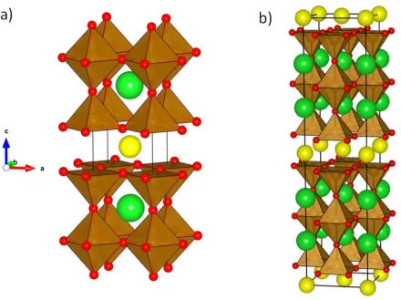
Chapter 1. Introduction
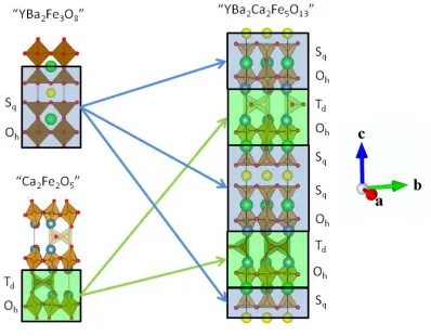
Figure 6 IdealisedYBa2Ca2Fe5O13 crystal structure15 (right), thought of as composed of blocks of the YBa2Fe3O8 and Ca2Fe2O5 structures11, 13, where the structural motif of each structure is represented by blue and green blocks respectivly. Atoms colours are as follows: yttrium (yellow), barium (green), calcium (blue), iron (brown) oxygen (red).
Chapter 1. Introduction
creation of three different cation sites, being 8, 10 and 12 coordinate and primarily occupied by Y, Ca and Ba respectively (Figure 6)
1.1.3 Magnetic ordering
Perovskites often containing transition metals on the B-site, can possess unpaired electrons which can lead to magnetic moments in the structure. Magnetic ordering between B-sites in perovskites has become an important consideration when performing ab-inito calculations in order to calculate accurate energies when unpaired electrons are present17. Spin polarisation in computational methods can be required when unpaired electrons are present (and therefore possibly magnetic structures) due to interaction energies being computed differently depending on whether or not spin polarisation is included18. Since all of the perovskites studied in this thesis contain transition metals on the B-sites magnetic ordering is relevant here to all of the systems here. Below is an overview of the types of magnetic states for solid systems relevant to the systems covered in this thesis.
Chapter 1. Introduction
Figure 7 Reported magnetic structure of MnO, where the magnetic unit cell has a lattice parameter twice that of the nuclear structure20, Manganese atoms coloured in purple, oxygen in red, with red and black representing differing spins.
Chapter 1. Introduction
Magnetic ordering in a system applies across a temperature range from 0 K upwards. At a certain temperature (material specific), magnetic coupling will break down, while the system still contains magnetic moments, there will be no overall magnetic ordering (known as a paramagnetic state), or in some cases different magnetic orderings can occur in different temperature regions. The temperature at which magnetic ordering breaks down is known as the Néel temperature (TN). In the paramagnetic state, each of the species with unpaired electrons possess a magnetic moment, but their spin states are not coupled and therefore are not ordered in the absence of an external magnetic field and so there is no overall magnetic moment in the system21.
Chapter 1. Introduction
Figure 8 Magnetic orderings discussed within this thesis, on a face centred unit cell containing 8 magnetic atoms in the asymmetric cell19, for clarity the symmetry equivalent atoms at the edges of the unit cell have been removed. a) Ferromagnetic, all of the spin moments are aligned in the same direction. b) A-type antiferromagnetic, spins are arranged in ferromagnetic sheets in the [100] plane. c) C-type antiferromagnetic, ferromagnetic sheets are aligned in the [110] direction. d) G-type antiferromagnetic, every atom has nearest neighbours with spin moments anti-aligned. The brown spheres represent arbitrary magnetic atoms.
Chapter 1. Introduction
The second type of antiferromagnetic ordering, C-type (Figure 8c), sheets of ferromagnetic ordering are observed in a diagonal crystallographic plane (e.g. [110]), with spin direction alternating between sheets. In systems with C-type antiferromagnetic ordering, each atom has four nearest neighbours with opposite spin directions (in plane with the atom) and two nearest neighbours with the same spin direction (above and below the plane).
The third type of antiferromagnetic ordering, G-type (Figure 8d), results in sheets of ferromagnetism that intersect all of the crystallographic planes (e.g. the [111] direction). G-type antiferromagnetic ordering results in magnetic atoms that have all nearest neighbours with opposite spin moments. G-type antiferromagnetic ordering is widely known in Fe containing perovskites, including all of the systems studied in this thesis12, 15, 22.
Chapter 1. Introduction
Chapter 1. Introduction
1.1.4 Phase Diagrams and solid solutions
When studying systems with multiple compositions, it is often convenient to map them out onto a phase diagram so as to be able to efficiently assess ranges of experimental conditions or stoichiometries and determine regions where single or multiple phases are observed to exist (Figure 10).
Figure 10 Phase diagrams from range of Y content in the YxBa3-xFe2MnO8 adapted from chapter 3 a) Representation from only the composition marking out regions according to the number of phases observed. b) Phase diagram representation with fractional quantities of each phase as a function of the Y content, with phase fractions obtained from powder diffraction data.
Chapter 1. Introduction
of where phase diagrams can be plotted in multiple dimensions, with the fraction of each phase as a function of yttrium content in the sample, where the system reaches an equilibrium between phases at each composition, with only a single point on the diagram favouring a single phase. Although in principle any number of additional dimensions can be included, accounting for a wide variety of parameters, including (but not limited to): plotting temperature against an oxygen partial pressure and mapping out the phase(s) observed in different regions24. Alternatively complex phase diagrams can be built up purely relating to the composition, in order to solely focus on which compositions can result in a single phase. For the example in Figure 10a, if one wanted to extend the investigation to include, YxBa3-xFe3-yMnyO8 a second axis would be added to the diagram indicating the Mn content and a similar plot produced with the number/type of phases observed in each region recorded. An example of this was critical in D. Hodgemans’ synthetic work in obtaining a phase pure composition following on from computational predictions presented in chapter 5 and the subsequent publication25.
Solid solutions of materials are the combination of two or more compounds synthesised into a single material, where a range of compositions can be formed into a single phase, typically given a form similar to C1-xDx, where C and D are two different compounds. Simple examples of an oxide solid solution include the reported solution between Fe2O3 and Cr2O3, to form the solution Fe2-xCrxO3 where x is reported between 0 and 2, with x values of 0.67, 1.00 and 1.33 explicitly
Chapter 1. Introduction
It is possible to construct solid solutions of more complex materials such as the perovskites discussed in the previous section (and becomes part of the focus of chapters 3 and 4), in order to create solid solutions both end members do not have to be known to exist or have the same structure type. An example of this is the doping of Co3+ into the aforementioned YBa2Fe3O8 material27, in order to form a solid solution of the form YBa2Fe3-xCoxO8. Where the first end
member is the 3ap, YBa2Fe3O8 and the other end member, YBa2Co3O8 is reported as a cubic perovskite with disordered oxygen vacancies30 and the 3ap structure is retained up to a nominal x value of 1.5 (50% substitution). This study also highlights the concept of a solid solution limit, i.e. an upper limit for the value of x, where a single phase material is formed, after which the compound at the solid solution limit crystallises out with remaining material crystallising as impurities. This strategy of doping materials by the formation of solid solutions can be used to tune the properties of a material, such as the d.c. conductivity or thermal expansion properties and has become an important method for the development of functional materials.
1.1.5 Doping perovskites and applications thereof
Chapter 1. Introduction
suppressing ferromagnetic ordering)37, the materials presented in chapters 4 and 5, are investigated within the research group as potential SOFC cathodes (with a schematic diagram of an SOFC cathode in Figure 11a).
Figure 11 a) Schematic representation of an SOFC fuel cell, adapted from38 with the corresponding overall reaction at the cathode shown in b)4
Therefore, for the overall reaction in (Figure 11b), a material should have a good electronic conductivity (experimentally demonstrated by d.c. conductivity/ area specific resistance (ASR)) and in order to promote the reaction only occurring at the surfaces of the material, to have the ability for oxygen ion conduction (typically demonstrated through ASR measurements), with materials containing both properties referred to as mixed-ionic-electronic-conductors (MIECs)38, with the parent material in chapter 4; Y1.1Ba1.5Ca2.3Fe5O13 shown to have good ASR values15 the d.c. conductivity is only modest.
Chapter 1. Introduction
including Ba1-xSrxFe1-yCoyO3-δ39-42. Since metal doping has been shown to tune the properties of oxide materials, chapter 3 investigates the principle of using ab-inito calculations to predict where doping will be possible and it is then applied the 10ap material in chapter 4 in order to guide synthetic efforts to improve the conductivity of the material. When several candidate sites are available, qualitative crystal chemical considerations may not always be capable of predicting the outcome of a substitution reaction, so in chapters 3 and 4 the concept of using ab-initio calculations to predict the outcome of site substitution in a structurally complex oxide is explored.
1.2
Theoretical calculations and solid state chemistry
As oxide research moves toward the discovery of new materials with increasing structural and compositional complexity, it is equally becoming more difficult to isolate such compounds by purely synthetic methods. Large and complex materials experimentally face two main problems, firstly, finding the composition at which a new structure can and will form for multiple element system can result in synthesis at a wide range of compositions and conditions with no guarantee that a new compound has not been missed. Secondly, even when new materials are formed, with large and complex structures, identifying the structure is a difficult task. Chapters 3 and 4 investigate the use of theoretical methods to calculate compositions at which new compounds can be formed, whereas chapter 5 focuses on using theoretical techniques to aid in the identification of a new complex oxide material.
Chapter 1. Introduction
calculations of band structures and corresponding density of states. The aid provided by theory covers a wide range of challenges utilising varying amounts of experimental information. At one end of the scale, where large amounts of experimental information is available are problems such as the most stable distribution of a set of cations for a given crystal structure and composition. At the opposite end, are problems where very little experimental information is known such as attempting to predict the contents of a compositional phase diagram in order to help guide future experimental synthesis. Although it should be noted that the level of experimental information available to use in the computational problem does not necessarily define problems complexity as the difficulty of the task is also reliant on the system size and number of different calculations required.
Given an infinite amount of computational power and infinite time, it would be possible to predict the structure of any compound by sheer brute force, i.e. to generate every possible permutation of a selection of atoms and to then calculate the corresponding free energy of every configuration. However in reality, in order to be able to perform calculations within a reasonable time frame and with the available computer resources, a number of different methods have been developed in order to efficiently aid experimental investigations. Although, each method either attempts to be as broad as possible or make a number of assumptions, resulting in limitations as to which systems a particular method can be applied to.
Chapter 1. Introduction
using modern computing resources, with the most suitable depending on the size of the system and what information is required.
In order to find a minimum energy structure, two things are required; a method by which to calculate the energy of the system and a method by which to alter the structure in order to search the energy landscape of the system43-46.
For calculating the energy of a system, there are three main levels of theory; ab-initio
calculations, classical mechanics and semi-empirical methods. With ab-initio calculations the energy of the system is computed with as few parameters as possible, with little information provided by the user apart from the atomic structure plus the number and type of atoms, with a common example of this being density functional theory (DFT, details given in the methods chapter). At the heavily parameterised end of theory is classical mechanics, whereby the energy of the system is calculated from completely parameterised atomic interactions also referred to as force fields (FF), a number of different types of force field are commonly used in simulation packages, details for the methods used in this thesis given in the methods chapter. In between these two types of theory are semi-empirical methods which combine elements from both of the above levels of theory. The most computationally expensive level of theory is the ab-initio
methods, with force fields being the cheapest and semi-emperical methods lying somewhere in-between depending on the level of parameterisation used. All of the calculations performed in this thesis fall into either classical mechanics or ab-initio, with a more detailed description presented in the experimental methods chapter.
Chapter 1. Introduction
To find the nearest minimum structure (also referred to as structure relaxation), the program may attempt to find the combination of inter-atomic distances that yields the lowest energy for example (assuming that each bond length will have an energy minimum as a function of distance). There exists a larger problem however; there is the possibility that the structure that is relaxed may not be the lowest possible energy structure for the system, i.e. it may be trapped into a local minima by large energy barriers preventing the energy minimisation finding it. However, relaxing a selection of local minima may be sufficient for specific systems, such as those studied in chapters 3 and 4. A number of levels of theory have been developed in order to find this lowest possible minimum structure, also known as the global minimum structure. In addition to attempting to approximate a brute force method, three common routines have been developed addressing the issue of finding the global minimum without resorting to the generation of as many structures as possible; Monte-Carlo sampling, molecular dynamics and genetic algorithms (which are discussed in the next section).
Chapter 1. Introduction
1.3
Applications of theory to solid state chemistry
1.3.1 Formation/Reaction energies and material doping
When synthesising solid solutions, it is desirable to be able to calculate regions where stable compositions are likely to exist and hence reduce the amount of compositional space that is searched experimentally. For some systems it has been possible to calculate formation energies in good agreement with experimentally determined values17, 48. The computation of solid solutions can be performed in at least two different ways. In the first method, formation energies are calculated from a library of relevant reference materials, so that balanced chemical equations can be found. For the second method energies can be computed relative to an ideal solid solution (if both end members are known to exist and reliable energies can be calculated). The energies of compositions are then calculated across the compositional range of interest and their energies compared to the required amounts of the end members to create balanced chemical equations.
The first method has been previously reported for the formation of ternary perovskites in the LaMO3 system from binary oxides and O2 gas17, the computed reaction energies compared with those experimentally reported in order to test the ability of DFT to correctly calculate reaction pathways, with an example given below for LaFeO3:
(1.3)
Chapter 1. Introduction
experiment. This methodology has also been previously reported for the calculation of a number of solid solutions48-51.
As the ability to be able to compute reaction energies has been established for some oxide systems the focus of the work presented in chapters 3 and 4 looks to utilise this capability. Firstly, formation energies are calculated for systems with larger unit cells than previously reported and containing a larger number of elements making for a complex challenge. The calculation of formation energies is used predicatively to guide the synthesis of the compounds presented to in chapters 3 and 4.
1.3.2 Convex hulls
52Convex hulls build on the calculation of formation/reaction enthalpies by calculating the minimum free energy43, 45 of formation with finite temperatures (including zero Kelvin) across a compositional range, with all of the results being mapped out onto a phase diagram, (such as the ternary phase diagram in Figure 12).
Chapter 1. Introduction
Once the library of known materials has been computed, hypothetical compositions are additionally inserted into the system and their corresponding free energy calculated. The energy of the system can be computed from any reasonable energy minimisation method, such as DFT or force fields, although the accuracy of the resulting phase diagram will vary with the accuracy of the energy minimisation. The free energy of the system can be calculated for any given finite temperature, including zero kelvin43 or a given range45.
Initially, the stability of each composition on the phase diagram is measured by the calculated free energy of formation relative to the components on the diagrams axes, with the free energies at each point resulting in a contour plot across the phase diagram52, referred to as the convex hull. Analysis of the convex hull will also allow for the identification of competing phases at each composition, based upon other compositions on the phase diagram that have similar or lower formation energies. The calculation of stability relative to competing phases allows one to predict whether the target phase is likely to form at a composition, or if it will react to form a mixture of other phases.
Chapter 1. Introduction
Figure 12 Adapted from43, a convex hull constructed for the Ce-Ir-In alloy phase diagram. Each point on the hull indicates a composition calculated, low energy structures are at the vertices of the intersecting lines. Point number 5, highlighted indicates the predicted and subsequently synthesised CeIr4In alloy material.
Chapter 1. Introduction
1.3.3 Data mining
Data mining is an approach for crystal structure prediction ,typically focused on finding experimentally unknown compositions that crystallise into previously known crystal structure types53, 54. Common methods by which data mining are implemented focus on calculating the ground state structure for a range of different compositions.
Chapter 1. Introduction
Figure 13 Adapted from55, results from the prediction of A2BX4 for X = Se, + signs indicate where unreported materials are predicted to be stable, - signs indicate compounds predicted to be unstable, ticks indicate known compounds and circles indicate compounds for which the computational methods remained undecided, grey boxes indicate compositions not trailled.
Data mining methods have the drawback however, that predictions can only be made for materials that possess a previously reported structure type. This type of approach has however been used to predict whole libraries of new materials that have yet to be discovered experimentally, exemplified by the prediction of a large number of unreported metal-chalcogenide materials predicted to be stable in the same study55 (Figure 13).
Chapter 1. Introduction
1.3.4 Molecular dynamics and simulated annealing
Molecular dynamics is a method to calculate the equilibrium structure of a compound at finite temperatures, rather than the lowest energy structure at zero Kelvin, these methods will allow for the calculation of structures as a function of temperature. Energy of the system is constantly updated in accordance with any of the energy calculation methods outlined above (i.e. ab-initio
or classical mechanics).
Atoms are moved using Newtonian physics, based upon the forces calculated between atoms to calculate momentum with time and at a finite temperature. The calculation proceeds as a function of time, with a user defined time step, typically on the order of femto-seconds. The forces and energy of the system are updated at each time step and the calculation is run for a user defined simulation length.
Chapter 1. Introduction
number of steps that are required to perform the calculation. Simulated annealing has resulted in the successful calculation of the global minimum of a number of structures46, 57, 58
1.3.5 Monte-Carlo
Figure 14 Example of a working Monte-Carlo routine (based upon a figure provided by M.S.Dyer, “rand” in the bottom right segment referrers to the random number generation between 0 and 1 for the probability that a higher energy structure will be accepted, with the routine typically run for either a pre-defined number of cycles or until a set number of steps rejected consecutively.
Chapter 1. Introduction
movement in the structure is performed, this can include moving one or more atomic positions or in a periodic system, varying the size/shape of the unit cell. The altered structure is then re-relaxed and a new energy calculated. If the new alteration to the structure is lower in energy then it is accepted. If the altered structure is found to be higher in energy the probability of it being accepted is calculated based upon a Boltzmann distribution dependent on the change in energy between steps and the probability is compared with a randomly generated number between 0 and 1, if it is less than the probability generated from the Boltzmann factor, it is accepted. Once the alteration is completed and the acceptance is determined, the cycle is repeated typically for a pre-determined number of cycles or until a user defined number of steps have been consecutively rejected.
1.3.6 Site disorder
In real solid state systems, there is often an amount of disorder on crystallographic sites, such as the disorder observed in the 10ap example in the previous section. It has been shown that cation disorder in oxides can result in lower overall energy configurations, even before considering entropy contributions15 and so for some systems it is important to be able to model this site disorder to obtain the lowest energy structure. For comparison between predicted and experimentally observed structures, the ability to estimate site disorder can decrease the difference between experimentally observed and calculated structures. Below, two separate methods for estimating site disorder for solid systems are discussed.
Chapter 1. Introduction
is little or no allowance for fractional occupancies of sites. A successful method to get around this problem has been reported and subsequently applied to investigate B-site cation disorder in the Ca2FeAlO5 brownmillerite59, where a large supercell of the material in question is generated in order to allow for statistical averaging across equivalent sites/atomic layers. Combined with the chosen method of energy minimisation, a Monte-Carlo routine is then applied for a fixed temperature, it differs from that presented above, in that instead of moving atomic positions/unit cell dimensions, each step consists of swapping pairs of non-equivalent atoms. This routine is then executed from the starting structure for a number of cycles until the lowest energy configuration is found, note that in order to eliminate very unlikely configurations it is possible to specify which atoms are allowed to swap places (e.g for a perovskite only allowing A-site species to swap with other A-site species). Once the minimum energy configuration is found from the starting structure, it is possible to then analyse each equivalent layer and estimate the fractional occupancies.
Chapter 1. Introduction
(1.4)
The starting point for the statistical mechanics approach is to compute the estimated free energy of each unique configuration, Em. Where Hm indicates the zero Kelvin energy calculated by a
chosen energy minimisation method and Sm is the calculated configurational entropy for the
configuration defined as:
(1.5)
Where kB is the Boltzmann constant and T is the finite temperature in Kelvin, which is then
multiplied by the natural log of the number of equivalent configurations that can are generated by the symmetry of the parent structure, Ωm. The expected population of a configuration m, Pm
can then be estimated for the system at thermal equilibrium:
(1.6)
Where Z indicates the partition function for the system, defined as:
m m B m T k E Z 1 exp (1.7)A modification to the method is used when considering materials containing magnetic atoms at high temperatures where is expected the system to be paramagnetic. In order to calculate the populations of materials expected to be paramagnetic at high temperatures, reports estimate a energy associated with the paramagnetic state as follows at zero K:
Chapter 1. Introduction
Where Hpm indicates the paramagnetic energy, HAF is the energy of the configuration in the
lowest energy antiferromagnetic ordering and HF indicates the energy of the configuration with
ferromagnetic ordering; the populations for each configuration are then calculated as described as above. The statistical mechanics approach is used as part of the calculations presented in chapter 3 and becomes an important measure of how well calculations can estimate site ordering for predicted crystal structures. The SOD method has also been used in the prediction of doping within oxide systems60, 61 as well as other systems49, 62-64, where in the methodology outline above, after the supercell has been generated a specified number of dopant atoms are then introduced before non-equivalent configurations are generated in order to calculate the most stable configuration across a solid solution. When dopant atoms are introduced, a pre-defined number of dopant atoms are introduced into the cell and then all of the possible configurations are generated using the symmetry of the parent undoped material.
Chapter 1. Introduction
not calculate occupancies at different temperatures, since the temperature factor used only affects the probability of higher energy structures being accepted.
1.3.7 Genetic Algorithms
Figure 15 Typical block scheme for an evolutionary algorithm, based upon the algorithm presented in65.
Chapter 1. Introduction
These methods begin with a population of starting configurations, often generated by random arrangements of atoms. During the run a maximum or fixed number of structures can be specified, whereby the first and subsequent generations of structures are constrained to these limits. The number of structures can vary in the system due to generated structures being outright rejected; for example in a periodic system a criterion could be for each lattice parameter to be larger than the diameter of the largest atom in the system in order to avoid unphysical structures. Each structure is usually then relaxed and then assessed for ‘fitness’ for a given set of criteria, for example by the calculated energy of the structure.
Once this process is completed a second generation of structures is created, known as the procreation step, by the combination of elements from a proportion of the structures that were considered to be the ‘fittest’ from the first cycle, with the allowance for random mutations of the structure (random displacement of a number of atoms for example). Again the new generation of structures is relaxed and then evaluated for their fitness and the procreation cycle is repeated again. The above cycles are repeated either for a pre-determined number of cycles or until the global minimum structure is obtained (defined by a set of convergence criteria).
This method of structure prediction has been shown in the literature to be able to successfully generate structures for oxide and mineral systems66-68 and computational packages designed specifically for the use of genetic and evolutionary algorithms with known energy minimisation techniques such as the USPEX44 code and has also been implemented in GULP66, 69, 70
Chapter 1. Introduction
advantage that it should eventually find the correct structure, and it is not limited to previously known structure types. Due to the number of generations and thus computational time that is often required the use of genetic algorithms tends to be restricted to smaller systems, although where it has been employed it has been proven to be an effective method by which to locate a global minimum structure.
1.3.8 Secondary building units
Chapter 1. Introduction
Figure 16 View of previously mentioned SrTiO3 broken down into two secondary building units (SBUs), this concept of breaking structures down into SBUs can be used to simplify the problem of generating complex structures, with this example, the SrTiO3 perovskite is broken down into AO layers (red) and BO2 layers (blue).
In this second example, large layered structures can be assembled from the stacking of these 2-D sheets and so it is possible to envisage utilising this concept in the assembly of large perovskite-like structures. For perovskites this would primarily originate from the alternation of AO and BO2 layers (from an ideal perovskite), and in order to be able to generate large perovskites such as those outlined previously oxygen vacancies would need to be included. This concept outlines the work undertaken in the discovery of a new layered perovskite presented in chapter 5.
Chapter 1. Introduction
When generating structures from SBUs, the resulting structures still require some form of energy minimisation, with the chosen method largely dependent on the number and size of the permutations that are generated. Once energy minimisation has been completed each of the permutations can then be ranked by their energy and the lowest energy structure determined.
1.4
Summary
In summary, there are wide choices of computational methods that can greatly assist experimental investigations, however, as outlined above, each technique has its own inherent drawbacks and therefore there is no one method that is universally applicable to every situation. Therefore when approaching a computational problem one should consider the following points before beginning:
What is the desired outcome of the investigation?
What level of experimental/computational information is available from which to build a starting point?
How many atoms/electrons and how many configurations are involved in the system?
Chapter 1. Introduction
the desired outcomes for the computational investigations were decided upon; in chapters 3 and 4, accurate enthalpies were required to predict stable compositions and the most likely structural configurations across a solid solution. In chapter 5, accurate energies were required in order to be able to predict the crystal structure of a unknown material. These aims meant that ab-initio
methods would have to be used in all three chapters.
Secondly, in chapters 3 and 4, it was decided that normal energy minimisation could be combined with the calculation of formation enthalpies since compositions and reasonable crystal structures were known, due to the chapters revolving around computational doping of known materials. For Chapter 5, however, only the approximate composition and unit cell size (and that the material was a perovskite) was known and so a method for finding the global minimum structure was required instead of normal energy minimisation. Due to the possible number of permutations for the atomic arrangements of the cell combined with prior knowledge about the crystal structure type, a method based on SBUs was developed, although if the crystal structure type was not known, it is likely that a combination of GA and simulated annealing methods may have been more appropriate.
Lastly, considering the size and number of the required configurations and available computing resources, it was decided that the relatively small number of configurations required for chapters 3 and 4 (on the order of tens to low hundreds) could all be completed using purely ab-initio
Chapter 1. Introduction
1.5
Aims of this thesis
Chapter 2 Synthetic and theoretical methods
Chapter 2.
Synthetic and theoretical methods
2.1
Solid state synthesis
All of the samples in this thesis were prepared via the standard ceramic methods76, 77. Prior to synthesis, the precursor materials were calcined to remove any moisture absorbed in the powder when stored at room temperature, in order to ensure that the correct stoichiometries are weighed out. Within this thesis and most starting materials were calcined at ~ 200 ˚C prior to weighing to evaporate any water contained in the powder, with the exception that Y2O3 was calcined at ~ 900 ˚C, due to Y2O3 being more hydroscopic than the other starting materials.
Once the starting oxides have been prepared, they were weighed out according to the stoichiometry required. Starting materials require mixing in order to ensure that the desired chemical reaction occurs efficiently and results in a homogenous product. The first step in mixing is to mill the starting powders; depending on the number of components and or the total amount of powder used, the starting materials can be milled by hand using a pestle and mortar or via a milling machine. Hand milling is typically suitable for smaller samples (a few grams) and larger samples milled mechanically. Mechanical milling has the advantage that it typically results in powders with smaller average particle sizes compared to hand milling. Consequently the finished samples can have higher densities, as is usually required for physical property measurements (e.g. d.c. conductivity measurements).
Chapter 2 Synthetic and theoretical methods
only improved mixing is required, after calcination, the sample is ground and re-mixed as described above.
Once the mixing and/or calcination step(s) have been completed, the chemical reaction is facilitated by a sintering step77. Sintering involves heating the sample to high temperatures (typically over 1000 ˚C for tens of hours), in order to allow the elements involved enough kinetic energy to diffuse through the sample and react. High temperature sintering is usually combined with pressing the sample into a pellet to increase contact between particles and therefore improve the solid state reaction rate. The sintering process often results in the sample density increasing significantly as particles fuse together in order to reduce the overall free energy of the system. For solid state reactions to form oxides, it is possible to adjust the atmosphere around the sample in order to manipulate the oxygen content and therefore the resulting product24; by either extracting oxygen from surrounding the sample with low oxygen partial pressures (e.g. by sintering the sample in a nitrogen flow), or at high partial pressures to attempt to increase the oxygen content with high oxygen partial pressures. In this thesis the concept of controlling the oxygen content in a sample becomes crucial to the successful synthesis of the target phase in chapter 3. It is common during the synthesis of oxide materials that a single sintering cycle does not provide enough energy, or inter-mixing to produce a single phase sample, and so several cycles of sintering and re-milling (also referred to as re-grinding) can be required.
Chapter 2 Synthetic and theoretical methods
2.2
Diffraction from crystalline solids
78The discovery that crystalline solids diffract x-rays was a critical in the field of material science as it now provides the basis for the identification of the atomic structure of crystalline materials. The idea that X-rays, having wavelengths similar to that of inter atomic spacings leads to the concept of solid lattices acting as a diffraction grating (with X-ray wavelengths having a magnitude of approximately 1 × 10⁻¹⁰ m or 1 Å) and was initially suggested by von Laue and confirmed by Friedrich and Knipping79. The original idea of X-ray diffraction was based from the concept that crystalline solids being 3-D arrays of atoms could act as a diffraction grating and from the way in which x-rays are diffracted information obtained about the atomic structure.
Figure 17 Schematic representation of Laue diffraction from a lattice in the x direction, where a is the lattice spacing, α0 and αn are the incident and diffracted x-ray beams, the path difference between adjacent beams is AB – CD.
Chapter 2 Synthetic and theoretical methods
z axis of the crystal respectively. Diffraction is observed when constructive interference occurs between diffracted X-ray beams from adjacent atoms (Figure 17) and the path length of neighbouring x-rays is integer multiples of the wavelengths which results in the following equation:
ABCD
Xi
cosncos0
ni (2.1)Where AB and CD are path lengths in (Figure 17), Xi denotes the atomic spacing along axis i (a,
b or c), αn and αi indicate the angles between the diffracted and incident beam, relative to the crystallographic axis i, ni indicates an integer multiple of wavelength, λ. Since diffraction can
occur with a component in each of the three axis; x, y and z, with the corresponding atomic spacing a, b or c equation (2.1) can be written for the diffraction component in each axis:
n
nxa cos cos 0 (2.2)
n
nybcos cos 0 (2.3)
n
nzc cos cos 0 (2.4)
Where angles βn, β0, and integer ny correspond to the angles and wave length multiples relative to
the y axis, likewise for γn, γ0 and nz for the z axis. The scheme in Figure 17, only illustrates
diffraction in the plane of the page, in reality, so long as the diffracted angle to the atomic row remains αn, then the diffraction conditions can still be met, this results in diffracted beams
actually forming a cone centred on the atomic row, with the apex of the cone having angle αn.
Chapter 2 Synthetic and theoretical methods
spacing and integers from equations (2.2 – 2.4) need to be determined. A simpler model was proposed by W. L. Bragg80, where diffraction was considered to be a reflection of the incident beam from planes of atoms (Figure 18), reducing the problem to two dimensions; although this is not physically correct, it makes geometrical sense, and substantially simplifies the problem.
Figure 18 Schematic representation of Bragg diffraction from planes of atoms, with the path difference between adjacent beams being (AB+BC), θ indicates the incident and diffracted beam angles and dhkl indicates the inter layer
spacing within the crystal with miller indices hkl.
From Braggs’ image of X-ray diffraction, the path difference between the beams scattered from adjacent planes of atoms, separated by the inter plane spacing dhkl is given by (2.5), where hkl
indicates the miller indices of the plane of atoms from which the x-ray beam is diffracting:
ABBC
(dhklsindhklsin)2dhklsin (2.5)For constructive interference to occur, the path difference has to equate to an integer number of wavelengths, resulting in the following condition for constructive interference:
2dhklsin
Chapter 2 Synthetic and theoretical methods
Where, n remains an integer number. Typically, experimentally collected diffraction patterns are plotted with observed intensity against the diffraction angle, 2θ, another common representation, especially when considering multiple data sets is Q, which is the momentum transfer on scattering and is defined by78:
hkl
d
Q
sin 2 4
(2.7)
For Braggs law, the separation of the atomic planes is the governing factor for constructive interference, rather than the specific atomic coordinates. The equations described above additionally show that Braggs description of x-ray diffraction, unlike von Laue’s, is only in two dimensions, dramatically reducing the number of parameters that require determination.
2.3
Powder Diffraction
81Chapter 2 Synthetic and theoretical methods
diffraction planes, as it is possible to have multiple crystallographic planes with equivalent dhkl
spacings, therefore regardless of the quality of the resolution of instrumentation, this overlap inevitably leads to an overall loss of information.
In spite of the inherent drawbacks of diffraction from powders, with the development of the Rietveld method78, 82-84, it has become possible to refine the crystal structure for polycrystalline materials successfully from powder diffraction data. As instrumentation has improved, combined with the introduction of powerful software packages for powder diffraction refinement, such as GSAS85, 86 or Topas87, 88, structure solution from powder diffraction data for even the most complex materials has become a reality, where previously structure solution could only originate from single crystal data.
X-ray diffraction is primarily used to solve the structure of crystalline materials, since amorphous materials are lacking in the regular repeating structure which results in a diffraction pattern. The interaction of the oscillating electric field of the incident x-ray beam interacting with electrons associated with the atoms in the material. X-ray diffraction analyses the X-rays scattered from the material retaining the incident beams wavelength. The observed dhkl values
Chapter 2 Synthetic and theoretical methods
To refine the structure from a powder diffraction pattern, a number of considerations are required, at least initially. The first observed fact is that the electron density for an atom falls very rapidly with increasing distance from the atoms centre. The assumed fall in electron density therefore leads to the conclusion that there is no overlap between neighbouring atoms. Secondly, it is assumed that the electron density for a given atom is spherically symmetrical. Lastly, each atom within a crystal structure of the same element type is assumed to have the same number of core electrons. This coupled with the assumption that bonding electrons do not contribute to scattering, results in the conclusion that the intensity of scattered X-rays from a given element is independent of the environment of the atom.
2.4
Laboratory based Powder X-ray Diffraction (PXRD)
78Chapter 2 Synthetic and theoretical methods
length. It is common however, for a metal target to have multiple characteristic emissions, with each emission being labelled according to the electronic state from which the electron is ejected (for example the most intense emission from a Cu target being labelled Kα1 radiation, with an s to p shell transition, with a wavelength of 1.54 Å).
Figure 19 Schematic representation of a Cu x-ray tube, adapted from78, when electrons pass from the filament (at high voltages), electronic excitations in the anode cause the release of x-ray photons, these x-rays pass through the Be window to the diffractometer optics and onto the sample.
Chapter 2 Synthetic and theoretical methods
experiment. A number of different geometries are commonly used in powder diffraction, with two being used within this thesis. The first is, known as Bragg-Brentano reflection78, the x-ray beam is diffracted from a sample held on a rotating flat plate (Figure 20a). The second geometry type is known as Debye-Scherrer transmission78, in which the sample is held in a rotating glass (typically borosilicate or silica) capillary of a known radius and is named geometry (Figure 20b). In both situations, the diffracted x-ray beam is typically detected by a moving detector (and/or sample) arm that will move through a 2θ range, on the circumference of the circle in Figure 20 measuring the diffracted intensity, thus generating the X-ray diffraction pattern.
Chapter 2 Synthetic and theoretical methods
2.5
Neutron Powder Diffraction (NPD)
78, 81Neutrons, like x-rays can have wavelengths with a magnitude similar to that of the inter-atomic spacing in crystalline materials, so it is also possible to perform diffraction experiments similar to those performed using X-rays. Unlike PXRD however, neutrons interact with the nucleus of an atom and therefore the technique is very sensitive to the atomic number, rather than electron number. As neutrons interact with the nucleus of an atom it makes it easier to observe lighter elements in the presence of metal atoms, thus making it an ideal technique for the study of oxides. Additionally diffracted neutrons do not have decreasing intensity with the scattering angle like x-rays do and so reflections with higher angles are easier to observe. Being able to measure smaller dhkl (higher θ) values compared to PXRD results in better refinement of
structural quantities that are dependent on the width of diffracted reflections (e.g. thermal parameters).
Since neutrons have an inherent spin moment, a neutron beam will interact with spin moments within a sample. It follows that if a sample has a magnetic ordering then, that a neutron diffraction pattern will have additional dhkl reflections and this allows for the identification of a
Chapter 2 Synthetic and theoretical methods
2.6
NPD at the ISIS neutron source on the High Resolution Powder
Diffractometer (HRPD)
89, 90Figure 21 Schematic of the ISIS neutron source, with all of the associated neutron diffraction instrumentation, adapted from figure presented on the STFC-ISIS webpage.
Chapter 2 Synthetic and theoretical methods
collide with a tungsten target, forcing an intra-nuclear cascade, resulting in neutron production. The resulting neutrons have a wide range of energies, the spread of neutron energies generated results in a range of wavelengths which can then be reduced by hydrogen containing moderators, typically water or methane. HRPD is a time of flight (TOF) diffractometer, utilising the entire range of wavelengths produced and therefore relying on solving Braggs law by utilising a continuum of wavelengths rather than diffraction angles, with the diffractometer using a bank of fixed detectors at known angles with respect to the sample. During a TOF experiment, the neutron wavelengths are calculated from the time taken for the neutrons to reach the detector from the source, with the relationship formalised in the following equation:
mL ht
(2.8)
where h is Planck’s constant, m is the mass of a neutron, L is the path length to the diffractometer and t is the time taken to reach the diffractometer. For the HRPD diffractometer (Figure 22), the moderator is methane which is maintained at 100 K. Any error caused by the neutron
Chapter 2 Synthetic and theoretical methods
Figure 22 Schematic for the HRPD instrument at the ISIS neutron source, adapted from90
2.7
Structure refinement
78, 81A refinement consists of computing the expected diffraction pattern from a model structure with the addition of functions to cover contributions to the pattern that are independent of the material, such as a pattern background from the sample holder. Once a pattern for the material is calculated, the differences between the theoretical and observed patterns are calculated. Refinements then take place, adjusting the structural or machine parameters in order to minimise the difference between the two, typically this is performed via a least squares routine78:
i
ci i i
y w y y
S 2 (2.9)
Where
i i
Chapter 2 Synthetic and theoretical methods
Where Sy is the total residual, wi is the weighting factor in order to normalise the residual for the
number of data points, yiindicates observed data points, yci indicates the calculated data points.
During the course of the refinement, a number of R factors can be used as a measure of how good the current fit is. The first R weighted pattern (referred to as Rwp), is often favoured as
there is no bias toward the structural model78:
2 1 2 2 ) (
i i ci i i wp y w y y w R (2.10)A second R factor, Rexp can also be calculated for a diffraction pattern, which can be deemed as
the best expected fit for the pattern78:
122 exp
wiyciP N
R (2.11)
Where N is the number of observations and P is the number of parameters being refined. Finally, at the end of a refinement, it is common to quote a ‘goodness of fit’ (GOF) or χ2 parameter, both of which related to the combination of Rwp and Rexp78:
2
exp 2 1
GOF
R R P N
Sy wp
(2.12)
Chapter 2 Synthetic and theoretical methods
from just accurate dhkl values to the refinement of the crystal structure; although in all methods,
(aside from simply assigning hkl values to reflections), refinement of parameters and functions that are machine dependant must be performed78, 81.
2.7.1 Background, zero shift and peak shape
In most refinement methods, there are three main factors to be accounted for. First is the diffraction pattern background, contributions to the background can come from the sample environment, such as the sample holder or depending on the wavelength an increased background may be observed for samples that fluoresce in the beam. Additionally, some samples will have a background component from structures which have local structures that deviate away from the long range average, or from amorphous phase fractions. Diffraction refinement software contain a number of different functions to fit the background of a diffraction pattern, such as the commonly used Chebechev polynomial function82.
Secondly, all diffractometers will have the some form of zero error, originating from such factors as the sample holders being misaligned, and is manifested in a uniform shift in all observed dhkl