Wide-Area Damping Controller of FACTS Devices for Inter-Area
Oscillations Considering Communication Time Delays
Wei Yao1,2, L. Jiang2, Jinyu Wen1, Q. H. Wu2, Shijie Cheng1
1State Key Laboratory of Advanced Electromagnetic Engineering and Technology, Huazhong
U-niversity of Science and Technology, Wuhan, 430074, China.
2Department of Electrical Engineering and Electronics, The University of Liverpool, Liverpool,
L69 3GJ, UK.
Abstract:The usage of remote signal obtained from a wide-area measurement system (WAMS) introduces time delays to a wide-area damping controller (WADC), which would degrade system damping and even cause system instability. The time delay margin is defined as the maximum time delay under which a closed-loop system can retain stable. In this paper, the delay margin is introduced as an additional performance index for the synthesis of classical WADCs for flexible AC transmission systems (FACTS) devices to damp inter-area oscillations. The proposed approach includes three parts: a geometric measure approach for selecting feedback remote signals, a residue method for designing phase compensation parameters, and a Lyapunov stability criterion and linear matrix inequalities (LMI) for calculating the delay margin and determining the gain of the WADC based on a trade-off between damping performance and delay margin. Three case studies are undertaken based on a four-machine two-area power system for demonstrating the design principle of the proposed approach, a New England 10-machine 39-bus power system and a 16-machine 68-bus power system for verifying the feasibility on larger and more complex power systems. The simulation results verify the effectiveness of the proposed approach on providing a balance between the delay margin and the damping performance.
Keywords: Wide-area damping controller, FACTS devices, inter-area oscillations, geometric ob-servability, time delays, delay margin.
1. Introduction
With the development of the wide-area measurement system (WAMS), remote signals have become available as the feedback signals to design wide-area damping controllers (WADC) for FACTS devices [36]. The availability of remote signals can overcome the aforementioned short-coming of lacking observability and provide flexibility to damp a special critical inter-area os-cillation mode of power systems [1], [7]- [14]. Various control techniques have been used to the design/synthesis of WADC, such as classical lead-lag phase compensation based control [1], robust control [9]- [11], adaptive control [12], model predictive control [13], and neural network based optimal control [14].
On the other hand, although WADCs provide a great potential to improve the damping of inter-area oscillation, the usage of remote signals also introduce a new challenge into the de-sign/synthesis of WADC, i.e., time delays caused by the usage of communication networks to transfer the remote signal will degrade the damping performance or may even cause instability of the closed-loop system [15, 18]. Those delays can typically vary from tens to several hundred mil-liseconds, depending on the distance, communication network, and protocol of transmission [16]-[17]. Moreover, calculation time of control law and faults of communication networks can also be converted into equivalent time delays [26]. However, most of these controllers mentioned above have not considered the influence of time delays introduced by the WAMS at the design stage.
Design of WADCs considering time delays have been addressed, such as applying nonlinear bang-bang control method to deal with time delays [37], designing robust controller to handle the time delay as a part of the system uncertainties [19]- [23], and compensating the time delays by designing a delay estimator [24]- [25]. On the other hand, delay-dependent stability analysis of WADC is investigated by calculating the maximal time delay (defined as delay margins) under which a power system equipped with a WADC can retain stable [26]. In [18, 27], delay-dependent stability analysis of load frequency control scheme and design of a robust load frequency controller by using delay margin as a new performance index are reported, respectively.
This paper proposes a systematic approach to design a WADC by introducing the delay mar-gin as an additional performance index and combining it with conventional design techniques to deal with communication delays, and apply it for design a WADC for FACTS devices in a multi-machine power system. The proposed approach consists of three steps, i.e., modal analysis and selection of feedback signals based on the geometric measures method [28, 29], design of the phase compensation part based on the residue method [1], and determination of controller gain based on trade-off between delay margin and damping performance. Case studies are undertak-en on a four-machine two-area power system, a New England 10-machine 39-bus power system, and a 16-machine 68-bus power system, respectively. The effectiveness of the proposed WADC is verified by simulation studies based on the detailed model.
This paper extends the work reported in [26] and its main contributions are summarized as follows:
• This paper concerns the design of a WADC for power system considering communication de-lays and proposes a systematic design approach for design of WADC by introducing the delay margin as an additional performance index into traditional control methods, while [26] mainly focuses on delay-dependent stability analysis of a power system equipped with a WADC.
• This paper generalizes the delay-dependent stability analysis method proposed in [26] and extends its application from analyzing WADC for generator exciter in [26] to a WADC for FACTS devices.
sys-tems for designing WADC of SVC. Moreover, calculation method proposed in [26] has been verified by designing WADC for SVC in a small and two relatively larger and complex test power systems, while reference [26] only investigates the four-machine two-area power sys-tem.
2. Design of a Wide-area Damping Controller Considering Time Delay
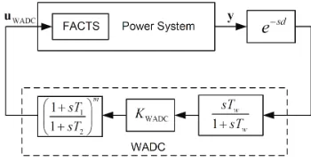
Overall structure of a WADC designed for a FACTS device is illustrated in Fig. 1. The WADC is designed to damp a critical inter-area oscillation mode by providing supplementary damping control signal for the FACTS device. A classical lead-lag type WADC is considered. The time delays existing in remote signals obtained from the WAMS, other sources such as sampling mea-surements and control law calculation are simplified as one single delaydat the feedback loop and represented by ae−sd block in Fig. 1.
As shown in Fig. 1, the transfer function of a classical WADC is:
HWADC(s) = KWADC
Tws 1 +Tws
(
1 +T1s
1 +T2s
)m
(1)
where T1 and T2 are phase compensation parameters; Tw is the washout constant and usually
chosen as5−10seconds;KWADCis the gain of the WADC;mis the number of the lead-lag block, usually,mis chosen to be2.
[image:3.612.217.392.394.485.2]The details of the proposed approach are described in the following subsections.
Fig. 1. The structure of a WADC for a FACTS device
2.1. Modal Analysis and Selection of Remote Feedback Signals
The dynamic model of power system is usually described by a set of differential-algebraic equa-tions (DAEs). The whole power system excluding the WADC can be linearized at an equilibrium
point as follows: {
˙
x(t) =Ax(t) +Bu(t)
y(t) = Cx(t) (2)
wherex ∈Rn×1, y ∈ Rq×1 andu ∈ Rp×1 are the vector of state variables, output variables and control variables, respectively; A ∈ Rn×n is the state matrix, B ∈ Rn×p the input matrix and
C ∈ Rq×nthe output matrix. Suppose matrix A has distinct eigenvaluesλ
k(k = 1,2, ..., n)and
the corresponding matrices of right and left eigenvectors, respectively,φandψ.
a suitable feedback signal for WADC, such as residue measures [29] and geometric measures [10, 28]. As the geometric measures can evaluate the comparative strength of a signal and the performance of a controller against to a given mode, this paper adopts geometric measures to design the WADC [29].
The geometric measures of controllability gmci(k)and observability gmoj(k)associated with
thekthmode are
gmci(k) = cos(α(ψk,bi)) = |
bT
i ψk|
||ψk||||bi||
(3)
gmoj(k) = cos(θ(φk,cTj)) =
|cjφk|
||φk||||cj||
(4)
wherebi theith column of input matrixB (corresponding to the ith input) andcj the jth row of
output matrix C (corresponding to thejth output). |z| and ||z|| are the modulus and Euclidean norm ofz, respectively;α(ψk,bi)is the geometrical angle between the input vectoriand thekth
left eigenvector, whileθ(φk,cTj)is the geometrical angle between the output vectorj and thekth
right eigenvector.
Since every control-loop may have significant effect to several low frequency modes, it is rec-ommended that the geometric observability measure should not be used as the only index for choosing wide-area control loop [38]. The joint controllability/observability measure (JCOM) is defined by
gmcok(i, j) =gmci(k)gmoj(k) (5)
The selected wide-area control loop should have large JCOM to the concerned critical inter-area mode, while small JCOM to other modes so as to reduce interaction to other modes. Therefore, the remote signal with the relatively large JCOM to the critical inter-area mode and relatively small JCOM to other inter-area modes should be selected as the input feedback signal.
2.2. Design of Phase Compensation Part
To achieve the damping of one oscillation mode, the eigenvalue corresponding to that mode must be placed at the left-half of the complex plane. This can be done by using phase compensation method described in [1]. Assumption Rkj is the residue of the transfer function Gj with regard
to thek-th mode, the amount of phase required compensationϕk, with regard to thekthmode, is
given by:
ϕk=π−argRkj (6)
Then the parameters of the lead-lag compensation part of WADC can be obtained by [30]:
α = T2 T1
= 1−sin(ϕk/m) 1 + sin(ϕk/m)
(7)
T1 =
1 2πfk
√
α, T2 =αT1 (8)
wherefkis the frequency of thekth mode.
2.3. Determination of Controller Gain
The delay-dependent criterion proposed in [26] is used to determine the delay margin of pow-er system embedded with a WADC and then the delay margin obtained will be used as a new performance index to design the WADC. The proposed approach includes the following steps: re-ducing the order of the power system excluding the controller, building up a closed-loop time-delay model, calculating delay margin of the closed-loop system and damp ratio of the concerned crit-ical inter-area mode, and finally obtain the controller gain based on a trade-off between damping performance and delay margin. By satisfying a given delay margin requirement, the gain of the WADC should be chosen as larger as possible in order to improve the damping performance of the closed-loop power system.
Based on the Schur model reduction method [31], the reduced-order system of the open-loop power system can be found as follows:
{ ˙
x1(t) = A1x1(t) +B1u(t)
y(t) = C1x1(t)
(9)
wherex1is the vector of state variables,A1the state matrix,B1the input matrix andC1the output matrix of the control system of the reduced-order power system.
The transfer function model of WADC shown in (1) should be converted to state-space model
as: {
˙
x2(t) = A2x2(t) +B2u2(t)
y2(t) = C2x2(t) +D2u2(t)
(10)
wherex2is the vector of state variables of the controller,y2 the vector of defined output variables,
u2the vector of control variables,A2the state matrix,B2the input matrix andC2the output matrix of the control system.
Thus, the model of the closed-loop power system considering time delay is obtained as:
˙
xc(t) = Acxc(t) +Adxc(t−d(t)) (11)
wherexc= [x1,x2]T, and
Ac=
[
A1 B1C2
0 A2
]
,Ad =
[
B1D2C1 0
B2C1 0
]
.
In a delay-dependent system, asymptotic stability holds for d < τd, whered denotes the time
delay andτdis the delay margin, and the system is unstable ford > τd. The delay marginτdis one
of the critical parameters for evaluating the stability of the delay-dependent system. Throughout this paper, the constant time delay is denoted asdand the time-varying delay is denoted asd(t), which is a continuous function of time and satisfies:
0≤d(t)≤τ, |d˙(t)| ≤µ≤1 (12)
whereτ andµare upper bounds of time delay and its rate, respectively. For a constant time delay,
µ= 0;d(t) = d = τ. For a time-varying delay,µ ̸= 0;τ andµare the upper bounds of the time delay and its rate, respectively.
margin. The problem of calculating the delay margin of (11) can be converted into a standard generalized eigenvalue minimization problem by using this method and then the delay margin can be found by using LMI functiongevpprovided in Matlab. The detailed description of this method is given in [26].
2.4. Summary of Steps of the Proposed Approach
Detailed steps of the proposed approach are summarized as follows:
Step 1: Building up a detailed model of the power system in MATLAB/Simulink and obtaining linear state-space model of the power system excluding the WADC at a chosen operating point by using Linear Analysis Toolbox provided in MATLAB.
Step 2: Carrying out modal analysis to find the frequencies and damping ratios of all low-frequency oscillation modes and identifying the critical inter-area mode.
Step 3: Selecting the feedback signal of the WADC based on the joint controllability/observability measure of candidate signals against to inter-area modes and choosing the one which has relative large geometric joint controllability/observability measure and less interactions to other inter-area modes.
Step 4: Determining the phase compensation parameters of the WADC by using the residue method.
Step 5: Obtaining the reduced-order model of the whole power system excluding the WADC using the Schur model reduction method [31], and obtaining reduced-order closed-loop system model including time-varying delay.
Step 6: Calculating the delay margins using the method described in [26] and damping ratios with regard to different gainsKWADC, respectively.
Step 7: Determining the gain of the WADC based on a trade-off between the damping perfor-mance and delay margin.
Step 8: Verifying the effectiveness of the designed WADC via simulation studies based on the original nonlinear detailed models.
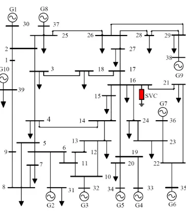
3. Case Study I: Four-machine Two-area System
To illustrate the principle of the proposed approach firstly, a case study is undertaken on the four-machine two-area benchmark system, as shown in Fig. 2. The test system consists of two areas connected by two parallel 220km long tie-lines between bus #7 and #9. Each area consists of two generators, each is equipped with a standard governor, automatic voltage regulator (AVR) and IEEE ST1A type static exciter. The generator is represented by a 6th-order sub-transient model. The load is modelled as constant impedance. Under nominal operating condition, approximately 400MW active power flows from Area 1 to Area 2. Both G1 and G3 are equipped with a PSS to damp the local mode oscillations. The detailed parameters of the system are given in [2].
Static VAR compensator (SVC), a common shunt compensation FACTS device widely used in power systems for improving voltage regulation, is chosen to be an example FACTS device [32]. As the voltage regulator of the SVC only provides small damping torque, it is necessary to augment a suitable WADC on the original control loop for improving the damping of inter-area oscillations [33]. The simulation studies are performed by using MATLAB/Simulink software.
Fig. 2. The four-machine two-area power system
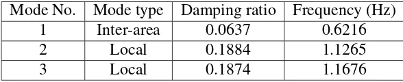
Table 1 Modal analysis results of the two-area system
Mode No. Mode type Damping ratio Frequency (Hz)
1 Inter-area 0.0637 0.6216
2 Local 0.1884 1.1265
3 Local 0.1874 1.1676
and has low voltage level. In addition, the main tie-lines of the large-scale interconnected power systems are also considered as a suitable location to install SVC. Thus, for this test system, a SVC with capacity±200MVar is installed at bus #8.
3.1. Modal Analysis and Selection of Feedback Signals
Modal analysis results of the test system are given in Table 1. It can be found that Mode #1 is an inter-area mode where generators in Area 1 are oscillating against generators in Area 2. As it has a relatively small damping ratio 0.0637 and oscillation frequency 0.6216Hz, it is considered as the critical mode whose damping is desired to be improved by the WADC of the SVC.
The geometric observability measures associated with Mode #1 are calculated and then used to choose the feedback signal of the WADC, as shown in Table 2. For simplification, the geometric observability measure are normalized so that the largest element is equal to1. As the rotor angle difference between G1 and G3δ1−3 has largest geometric observability index, it is chosen as the remote feedback signal of the WADC.
Table 2 Geometric observability measure associated with Mode #1 of the two-area system
No. Signal candidates Geometric observability measure
1 δ1−3 1.0000
2 I7−8 0.9564
3 δ2−3 0.9377
4 δ1−4 0.9260
5 P7−8 0.8688
6 I8−9 0.8676
7 P8−9 0.8633
8 δ2−4 0.8633
9 I6−7 0.6421
[image:7.612.157.457.557.716.2]10−1 100 101 102 −90
−80 −70 −60 −50 −40 −30 −20 −10 0 10
Frequency (rad/s)
Magnitude (dB)
Full order
[image:8.612.210.395.87.225.2]9th order 8th order
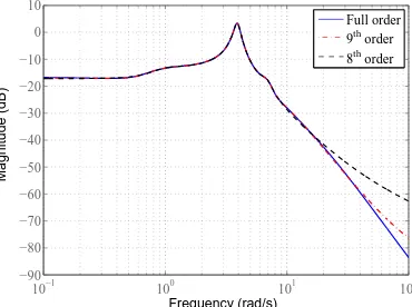
Fig. 3. The frequency responses of the full-order and the reduced-order model of the two-area system
3.2. Model Order Reduction
The open-loop system excluding the WADC is a43thorder system. With choosingδ
1−3as output anduWADC as input, the Schur balanced model reduction method is adopted [26]. The frequency responses of the reduced-order systems with different order and the full-order system are shown in Fig. 3. It can be found that when the model order is more than8, the frequency response of the reduced-order system is very close to that of the full-order system over the frequency range from
0.1rad/s to50rad/s, which covers the concerned low-frequency oscillation range between0.2and
2.5Hz. Hence, the 9th-order system is used for calculating the delay-margin of the closed-loop system.
3.3. Design of the WADC
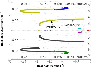
The residue value obtained from the modal analysis of Mode #1 is0.0072 + 0.3637i. According to (7) and (8), the parameters of lead-lag compensation part of the WADC are given as: Tw = 10s,
T1 = 0.6096s, and T2 = 0.1075s. The root locus of the closed-loop system without considering time delays is shown in Fig. 4. WhenKWADCincreases, the damping ratio of the critical inter-area Mode #1 increases. It can be concluded that the gain of the WADCKWADC is the key parameter related with the damping performance of the Mode #1. To avoid an excessive interference of the main voltage regulator, the output of the WADC is limited by±0.1pu [2].
Based on the 9th-order system model, the delay margin τ
dwith respect to different sets of the
gainKWADC and the delay rateµare calculated and summarized in Table 3. As same as in [26], we find that τd decreases with the increase of KWADC. Moreover, for a fixed gain KWADC, τd
decreases with the increasing of µ. The relationship between damping ratio of Mode #1 and the gain of WADC is also given in Table 3, which shows that damping ratioξof the Mode #1 increases with the increasing ofKWADC. In summary, with the increase of theKWADC, the damping ratioξ increases while the delay marginτddecreases and vice versa. Therefore, theKWADCcan be tuned based on a trade-off between the damping performance and the delay margin.
−3 −2.5 −2 −1.5 −1 −0.5 0 −10
−5 0 5 10
0.025 0.055 0.085 0.125 0.18 0.25
0.38
0.65
0.025 0.055 0.085 0.125 0.18 0.25
0.38 0.65
2 4 6 8 10
2 4 6 8 10
Real Axis (seconds−1)
Imaginary Axis (seconds
−1
)
[image:9.612.207.394.87.226.2]Kwadc=0.20 Kwadc=0.70
Fig. 4. The root locus of the closed-loop two-area power system (KWADC: 0−3.0)
Table 3 Delay margin and damping ratio of Mode #1 with respect to differentKWADCof Case I
τd/ms [9th order] Mode #1
KWADC µ= 0 µ= 0.5 µ= 0.9 ξ f (Hz)
0 — — — 0.0637 0.6216
0.12 505.5 503.4 503.4 0.1264 0.6164 0.15 451.9 451.9 451.9 0.1418 0.6145 0.20 399.8 399.8 399.8 0.1673 0.6108 0.30 338.9 329.7 302.4 0.2173 0.6012 0.50 248.6 194.8 194.2 0.3138 0.5741 0.70 158.3 152.8 152.8 0.4020 0.5365 1.00 123.9 111.7 102.8 0.5043 0.4734
KWADC changes from 0.7 to 0.2, the damp ratio is reduced from 0.4020 to 0.1673 but with a significant increase of delay margin from158.3ms to399.8ms. As the time delay of the wide-area signal can typically vary from tens to several hundred milliseconds, the gainKWADC = 0.2should be chosen for the WADC so that the closed-loop system has a large delay margin but still provides satisfactory damping performance.
3.4. Simulation Evaluation
Simulation studies are carried out based on the detailed model to verify the effectiveness of the proposed approach. The small disturbance applied for the case study is that the reference of G1 terminal voltage increases+5%att = 1s.
The system responses of the WADC withKWADC = 0.7and withKWADC = 0.2under different time delays existing in the wide-area signal, are shown in Fig. 5 and Fig. 6, respectively. Without time delays, both WADCs can damp out the critical inter-area Mode #1 effectively and provide almost similar damping performances.
When the time delay is increased to180ms, the WADC with gainKWADC= 0.7cannot maintain system stability since time delay exceeds its delay margin158.3ms. However, the WADC with gain
[image:9.612.164.447.278.426.2]0 5 10 15 20 −1.5 −1 −0.5 0 0.5 1 1.5x 10
−3
Time (sec)
Rotor speed (G
1 −G 4 ) (rad/s) d=0ms d=180ms NO WADC
0 5 10 15 20 0.25 0.3 0.35 0.4 0.45 Time (sec)
Rotor angle (G
[image:10.612.182.422.73.164.2]1 −G 3 ) (rad) d=0ms d=180ms NO WADC
Fig. 5. The responses of the two-area system with increasing+5%voltage reference of G1 under different time delays (KWADC = 0.7)
0 5 10 15 20 −1.5
−1 −0.5 0 0.5
1x 10
−3
Time (sec)
Rotor speed (G
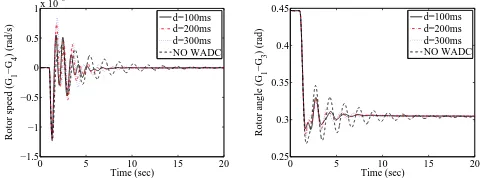
1 −G 4 ) (rad/s) d=100ms d=200ms d=300ms NO WADC
0 5 10 15 20 0.25 0.3 0.35 0.4 0.45 Time (sec)
Rotor angle (G
1 −G 3 ) (rad) d=100ms d=200ms d=300ms NO WADC
Fig. 6. The responses of the two-area system with increasing+5%voltage reference of G1 under different time delays (KWADC = 0.2)
margin 399.8ms based on Table 3. This simulation results verify the gainKWADC = 0.2should be determined for the WADC as the closed-loop system has a large delay margin and a satisfactory damp performance.
4. Case Study II: New England 10-machine 39-bus System
To investigate the feasibility of the proposed approach at a complex power system, a case study is undertaken based on the New England 10-machine 39-bus system, as shown in Fig. 7. This test system is a typical inter-connected system with poorly damped inter-area oscillation modes and has been widely used for studying the low frequency oscillation [10]. It consists of10generators,
39buses, and46transmission lines. Each generator is modeled as a4th-order model and equipped with a IEEE DC1A excitation system, except generator G10 which is an equivalent infinite unit. The transmission system is modeled as a passive circuit and the loads are modeled as constant impedances. The mechanical power of each generator is assumed as constants for simplicity. The detailed parameters and operating conditions are given in [34]. The transmission lines between bus
#15and#16, bus#16and#17are the inter-area tie-lines which divide the entire system into two sub-systems. For this test system, since bus#16is the bus with low voltage profile, a±500Mvar SVC is installed at the bus#16to support the voltage profile.
4.1. Modal Analysis and Selection of Feedback Signals
[image:10.612.181.424.219.308.2]Fig. 7. The New England 10-machine 39-bus power system
Table 4 Modal analysis results of the New England system
Mode No. Mode type Damping ratio Frequency (Hz)
1 Inter-area 0.0592 0.6093
2 Inter-area 0.0394 0.9310
3 Inter-area 0.0432 1.0390
4 Local 0.0445 1.1430
5 Local 0.0373 1.2735
6 Local 0.0378 1.4190
7 Local 0.0549 1.4658
8 Local 0.0442 1.5080
9 Local 0.0745 1.5110
#2 to #9 are small, they have relatively large frequency values. Thus the oscillation related with those modes will decay quickly and it is not necessary to provide supplementary damping control for those modes [10]. Therefore, the WADC of the SVC will be designed mainly for increasing the damping of the critical inter-area Mode #1, which has relatively small damping ratio 0.0592and low oscillation frequency0.6093Hz.
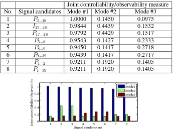
Table 5 and Fig. 8 show the JCOM of the wide-area signals to inter-area Mode #1, #2, #3. All JCOM values are normalized by using the largest JCOM as the based value. In Table 5,Ii−j
represents the magnitude of current between bus #iand #j andPi−j the active power between bus
#i and #j. P3−18 is selected as the feedback signal for the WADC because it not only has the relatively large JCOM ( at this case, it is the largest) to Mode #1 but also relatively small JCOM to Mode #2 and #3, among all candidates shown in Table 5.
4.2. Model Order Reduction
[image:11.612.155.455.330.480.2]Table 5 Joint controllability/observability measure associated with Mode #1,#2,#3, of the New England system
Joint controllability/observability measure No. Signal candidates Mode #1 Mode #2 Mode #3
1 P3−18 1.0000 0.1450 0.0975
2 I17−18 0.9844 0.4439 0.1532
3 P17−18 0.9792 0.4429 0.1517
4 P5−8 0.9543 0.1427 0.2333
5 P8−9 0.9450 0.1417 0.2718
6 P9−39 0.9439 0.1417 0.2717
7 P1−2 0.9211 0.1920 0.1405
8 P1−39 0.9211 0.1920 0.1405
1 2 3 4 5 6 7 8
0 0.2 0.4 0.6 0.8 1
Signal candiates no.
Joint controllability/observability
[image:12.612.212.396.397.534.2]Mode1 Mode2 Mode3
Fig. 8. Joint controllability/observability measure associated with Mode #1-#3
10−1 100 101 102
−5 0 5 10 15 20 25 30
Frequency (rad/s)
Magnitude (dB)
Full order 9th order 8th order
Fig. 9. The frequency responses of the full-order and reduced-order model of the New England system
applied. Comparing the frequency responses of the reduced-order with the full-order model shown in Fig. 9, the reduced model is determined as 9th-order because it can provide similar frequency
response with that of the full-order system over the concerned oscillation frequency range between
0.2and2.5Hz.
4.3. Design of WADC
Table 6 Delay margin and damping ratio of Mode #1 with respect to differentKWADCof the New England system
τd/ms [9th order] Mode #1
KWADC µ= 0 µ= 0.5 µ= 0.9 ξ f (Hz)
0 — — — 0.0592 0.6093
0.008 448.2 399.5 350.5 0.1213 0.6126 0.009 352.2 275.8 244.0 0.1290 0.6113 0.010 233.8 162.8 138.9 0.1366 0.6142 0.011 90.4 53.9 45.0 0.1441 0.6160 0.012 70.9 47.4 31.7 0.1515 0.6182 0.013 60.2 42.4 29.1 0.1586 0.6208 0.015 47.2 35.0 24.9 0.1718 0.6272 0.020 31.2 24.4 18.3 0.1932 0.6509
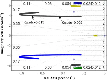
T1 = 0.6823s, and T2 = 0.1000s. The root locus of the closed-loop system without considering time delay is shown in Fig. 10. WhenKWADC changes from0to0.015, the damping ratio of the Mode #1 increases significantly from0.0592to0.1718. To avoid the excessive interference of the main voltage regulator, the output of the WADC is limited by±0.1pu [2].
−0.8 −0.6 −0.4 −0.2 0
−6 −4 −2 0 2 4
6 0.11 0.08 0.054
0.17
0.35
0.012 0.024 0.038 0.054 0.08 0.11
0.17 0.35
1 2 3 4 5 6 7
1 2 3 4 5 6 7 0.012 0.024 0.038
Real Axis (seconds−1)
Imaginary Axis (seconds
−1
)
Kwadc=0.015 Kwadc=0.009
Fig. 10. The root locus of the closed-loop New England power system (KWADC : 0−0.05)
Based on the9th-order model, the delay marginsτ
dwith respect to different gainsKWADCand the delay rateµare calculated and shown in Table 6. The damping ratio of Mode #1 under different gains are given in Table 6 as well. The relationship between gains and delay margins are as similar as as the simple case can be obtained.
As shown in Table 6, when KWADC reduces from 0.015 to 0.009, the damping ratio reduces from0.1718to0.1290, while the delay margin increases significantly from47.2ms to352.2ms. Therefore, the gainKWADC = 0.009is determined for the WADC such that the closed-loop system has a large delay margin but still provides satisfactory damping performance.
4.4. Simulation Evaluation
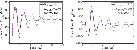
[image:13.612.210.394.344.482.2]0 2 4 6 8 10 0 100 200 300 400 500 Time (sec)
Active Power P
16−15
(MW)
KWADC=0.015 KWADC=0.009
NO WADC
0 2 4 6 8 10 −300 −200 −100 0 100 200 300 Time (sec)
Active Power P
3−18
(MW)
KWADC=0.015 KWADC=0.009
[image:14.612.183.424.76.165.2]NO WADC
Fig. 11. The responses of the New England power system to fault with different gains of the WADC
0 2 4 6 8 10 0 100 200 300 400 500 Time (sec)
Active Power P
16−15
(MW)
d=0ms d=65ms NO WADC
0 2 4 6 8 10 −0.1 −0.05 0 0.05 0.1 0.15 Time (sec)
Output of WADC (p.u)
[image:14.612.181.423.207.293.2]d=0ms d=65ms NO WADC
Fig. 12. The responses of the New England power system to fault with different time delays (KWADC = 0.015)
0 2 4 6 8 10 0 100 200 300 400 500 Time (sec)
Active Power P
16−15 (MW) d=300ms d=200ms d=100ms NO WADC
0 2 4 6 8 10 −0.1 −0.05 0 0.05 0.1 0.15 Time (sec)
Output of WSDC (p.u)
d=300ms d=200ms d=100ms NO WADC
Fig. 13. The responses of the New England power system to with different time delays (KWADC =
0.009)
responses of the system are shown in Fig. 11. It is shown that the WADC can provide effective damping of inter-area oscillations and the WADC with gain KWADC = 0.015 provides slightly better damping performance than the WADC with gainKWADC = 0.009. This is also confirmed by the root locus of the closed-loop system shown in Fig. 10.
The system responses of the WADC with different time delays existing in the wide-area signal are shown in Fig. 12 and Fig. 13, respectively. When the time delay reaches to65ms, the WADC with gainKWADC= 0.015cannot maintain system stability as the time delay exceeds its delay mar-gin47.2ms, according to Table 6. However, the WADC with gainKWADC = 0.009 can damp out the critical inter-area Mode #1 effectively even with the time delay as large as300ms. Moreover, when the time delay varies from 100ms to 300ms, the WADC with gain KWADC = 0.009 pro-vides almost similar damping performance. This is because the WADC with gainKWADC= 0.009 has a large delay margin 352.2ms, as shown in Table 6. This simulation results verify the gain
KWADC = 0.009should be determined for the WADC as the closed-loop system has a large delay margin but still provides good damp performance.
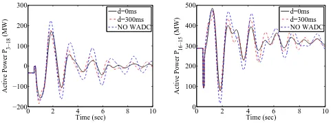
[image:14.612.178.423.351.440.2]0 2 4 6 8 10 −200 −100 0 100 200 300 Time (sec)
Active Power P
3−18
(MW)
d=0ms d=300ms NO WADC
0 2 4 6 8 10 0 100 200 300 400 500 Time (sec)
Active Power P
16−15
(MW)
[image:15.612.182.424.75.165.2]d=0ms d=300ms NO WADC
Fig. 14. The responses of the New England power system to fault followed by outage of line #3-#4 (KWADC = 0.009)
0 2 4 6 8 10 −300 −200 −100 0 100 200 Time (sec)
Active Power P
3−18
(MW)
d=0ms d=300ms NO WADC
0 2 4 6 8 10 100 200 300 400 500 600 Time (sec)
Active Power P
16−15
(MW)
d=0ms d=300ms NO WADC
Fig. 15. The responses of the New England power system to fault when active power of tie-line is
670MW (KWADC= 0.009)
re-closed after the fault is cleared. Scenario II is that the total power flow of tie-lines (line #16-#15 and #16- #17) increases from 494MW to 670MW. Fig. 14 and Fig. 15 illustrate the sys-tem responses to Scenario I and Scenario II, respectively. It can be concluded that the proposed WADC can provide enough damping to the system and has satisfactory robustness against different operating conditions.
5. Case Study III: 16-machine 68-bus System
To further investigate the feasibility of the proposed approach in a more complex and realistic power system, design of WADC for SVC in a 16-machine 68-bus test system shown in Fig. 16 is given in this section. This system is a simplified New England and New York interconnected system and has been used to test the effectiveness of WADC in a relatively large power system [39, 40]. All generators are modeled via a 6th-order model, the governor dynamics are neglected while the IEEE ST1A excitation system is adopted for G1-G15, and all loads are represented as constant impedance. In addition, the PSS is equipped at G1-G12 to provide damping for local and inter-area oscillation modes. The detailed description of this test system including network data, parameters of generators and excitation systems are given in [39]. For this test system, a ±600Mvar SVC is installed at the bus#51to maintain its voltage profile.
5.1. Modal Analysis and Selection of Feedback Signals
[image:15.612.183.424.220.309.2]objec-Fig. 3. 5-area, 16-machine, 68-bus system.
[image:16.612.186.428.73.252.2]Fig. 16. The 16-machine 68-bus power system
Table 7 Modal analysis results of the 16-machine 68-bus system
Mode No. Mode type Damping ratio Frequency (Hz)
1 Inter-area 0.1332 0.3791
2 Inter-area 0.0316 0.5365
3 Inter-area 0.1636 0.6585
4 Inter-area 0.0519 0.7957
tive is to design a WADC to provide damping to Mode #2, which has relatively lower frequency and the smallest damping ratio.
Fig. 17 and Table 8 show the JCOM of different wide-area signal candidates with respect to four inter-area modes. As shown in Table 8 and Fig. 17, the signal 1 (P46−38) has the largest JCOM to the Mode #2, but also has relatively large JCOM to the Mode #1, which represents a potential modes interactions. The signal 5 (P68−52) has smaller JCOM to Mode #2 than signal 1, but JCOM to all other modes are relatively small. Therefore, signal 5P68−52is selected as the feedback signal for the WADC because it not only has the relatively large JCOM among these candidates but also has smaller interaction to other three inter-area modes. Note that signal 2 and signal 6 represent current magnitude and are correlated closely to signal 1 and signal 5, respectively.
1 2 3 4 5 6 7 8
0 0.2 0.4 0.6 0.8 1
Signal candidate no.
Joint controllability/observability
[image:16.612.158.455.307.382.2]Mode1 Mode2 Mode3 Mode4
[image:16.612.193.412.553.653.2]Table 8 Joint controllability/observability measure associated with Mode #1,#2,#3,#4, of the 16-machine 68-bus system
Joint controllability/observability measure No. Signal candidates Mode #1 Mode #2 Mode #3 Mode #4
1 P46−38 0.6769 1.0000 0.2000 0.0925
2 I46−38 0.6227 0.9665 0.1844 0.0818
3 I1−31 0.0851 0.5659 0.4907 0.0197
4 P1−31 0.0882 0.5094 0.4711 0.0186
5 P68−52 0.0483 0.3724 0.0475 0.1180
6 I68−52 0.0576 0.3569 0.0488 0.1097
7 P31−30 0.2319 0.1747 0.1670 0.0548
8 I31−30 0.2402 0.1671 0.1806 0.0577
10−1 100 101 102
−10 −5 0 5 10 15 20 25 30 35
Frequency (rad/s)
Magnitude (dB)
Full order 8th order
7th order
Fig. 18. The frequency responses of the full-order and reduced-order model of the New England system
5.2. Model Order Reduction
Via choosing the deviation of active powerP68−52as the output anduWADC as the input, the Schur reduction method is applied to obtain a reduced-order model of the original133thorder test system. Comparing the frequency responses of the reduced-order system with the full-order model over the concerned oscillation frequency range between 0.2 and2.5Hz, as shown in Fig. 18, the order of the reduced model is determined as8th-order.
5.3. Design of WADC
For Mode #2, the residue value obtained from the linearized analysis is 2.0877 + 4.0014i. Ac-cording to (7) and (8), the parameters of lead-lag compensation part are obtained as: Tw = 10s,
−0.8 −0.7 −0.6 −0.5 −0.4 −0.3 −0.2 −0.1 0 0.1 −6
−4 −2 0 2 4 6
0.012 0.026 0.042 0.062 0.09 0.13
0.2
0.4
0.012 0.026 0.042 0.062 0.09 0.13
0.2 0.4
1 2 3 4 5 6
1 2 3 4 5 6
Real Axis (seconds−1)
Imaginary Axis (seconds
−1
)
[image:18.612.209.396.87.226.2]Kwadc=0.013 Kwadc=0.025
Fig. 19. The root locus of the closed-loop 16-machine power system (KWADC : 0−0.03)
Table 9 Delay margin and damping ratio of Mode #2 under differentKWADCof Case III
τd/ms [8th order] Mode #2
KWADC µ= 0 µ= 0.5 µ= 0.9 ξ f (Hz)
0 — — — 0.0316 0.5365
0.008 441.9 389.0 336.8 0.0559 0.5515 0.010 348.3 320.2 228.7 0.0636 0.5554 0.013 284.3 241.1 188.4 0.0768 0.5612 0.015 252.4 190.7 168.0 0.0869 0.5651 0.020 186.1 130.4 120.4 0.1198 0.5733 0.025 86.4 55.0 35.5 0.1643 0.5712 0.026 41.4 32.6 21.6 0.1722 0.5691
Based on the8th-order reduced model, the delay marginsτd under different gainsKWADC and different delay rates µare calculated and shown in Table 9. The damping ratio ξ and frequency
f of Mode #2 under different gainsKWADC are also calculated and given in the last two columns of Table 9. Similar relationship between gains and delay margins can be obtained as Case Study I and II.
As shown in Table 9, when KWADC reduces from 0.025 to 0.013, the damping ratio reduces from0.1643to0.0768, while the delay margin increases significantly from86.4ms to284.3ms. Therefore, to provide a delay margin in the range between250ms and400ms, the gainKWADC =
0.013should be chose with the cost of reduction of damping ratio from0.1643to0.0768.
5.4. Simulation Evaluation
Simulation studies are carried out based on detailed nonlinear model to verify the effectiveness of the designed WADC. A three-phase-to-ground fault occurs at the end terminal of line #45- #51 near bus #45 att = 0.5s and is cleared at t = 0.6s. When there is no time delay existing in the wide-area signal, the responses of the system are shown in Fig. 20. It is shown that the WADC can provide effective damping of inter-area oscillations and the WADC with gainKWADC= 0.025 provides slightly better damping performance than the WADC with gainKWADC = 0.013. This is also confirmed by the root locus of the closed-loop system shown in Fig. 19.
[image:18.612.164.449.278.426.2]are shown in Fig. 21 and Fig. 22, respectively. When the time delay reaches to100ms, the WADC with gainKWADC = 0.025 cannot maintain system stability as the time delay exceeds its delay margin86.4ms, according to Table 9. However, the WADC with gainKWADC = 0.013can damp out the critical inter-area Mode #1 effectively even with the time delay as large as250 ms. This is because the WADC with gain KWADC = 0.013 has a large delay margin 284.3ms, as shown in Table 9. Therefore, the gain KWADC = 0.013 should be determined for the WADC as the closed-loop system has a large delay margin but still provides good damp performance.
0 5 10 15
3700 3800 3900 4000 4100 4200 4300 4400 Time (sec)
Active Power P
68−52
(MW)
KWADC=0.013 KWADC=0.025
NO WADC
0 5 10 15
30 40 50 60 70 80 90 100 110 Time (sec)
Active Power P
46−38
(MW)
KWADC=0.013 KWADC=0.025
[image:19.612.182.423.184.270.2]NO WADC
Fig. 20.The responses of the 16-machine power system to fault without delay under different gains of the WADC
0 5 10 15
3700 3800 3900 4000 4100 4200 4300 4400 Time (sec)
Active Power P
68−52
(MW)
KWADC=0.013
KWADC=0.025 NO WADC
0 5 10 15
30 40 50 60 70 80 90 100 110 Time (sec)
Active Power P
46−38
(MW)
KWADC=0.013
[image:19.612.182.423.338.427.2]KWADC=0.025 NO WADC
Fig. 21. The responses of the 16-machine power system to fault with100ms delay under different gains of the WADC
0 5 10 15
3700 3800 3900 4000 4100 4200 4300 4400 Time (sec)
Active Power P
68−52
(MW)
d=150ms d=250ms NO WADC
0 5 10 15
30 40 50 60 70 80 90 100 110 Time (sec)
Active Power P
46−38
(MW)
d=150ms d=250ms NO WADC
Fig. 22. The responses of the 16-machine power system to fault under different time delays (KWADC = 0.013)
6. Conclusion
[image:19.612.183.422.494.579.2]performance index and combines with the geometric measure method for selecting the feedback input signal and the residue method to design the phase compensation part of the WADC.
The delay margin is calculated by a Lyapunov stability criterion and linear matrix inequalities (LMI), based on the reduced-order model of the large-scale power system excluding the WADC. The gain of the WADC is a key parameter related with the delay margin and the damping per-formance: the increase of the gain of WADC will reduce the delay margin, while increase the damping ratio of the critical inter-area oscillation mode. Based on a tradeoff between the damp-ing performance and the delay margin, the gain should be chose either to provide a satisfactory damping performance while with a larger delay margin, or as larger as possible to enhance the damping performance after the delay margin obtained from practical requirement is satisfied. The design of a classical lead-lag type WADC for SVC-type FACTS devices has been carried out by three case studies based on the four-machine two-area power system, the New England 10-machine 39-bus power system, and 16-machine 68-bus power system, respectively. Results of the case s-tudies have verified the effectiveness of the proposed approach to achieve a compromise between damping performance and delay margin, and demonstrated the feasibility of its applications in a relatively large-scale power system.
Further studies will focus on coordinating design and tuning of WADCs for damping multiple inter-area oscillation modes by using results of the delay-dependent stability analysis of the power system with multiple time-varying delays.
7. References
[1] M. E. Aboul-Ela, A. A. Sallam, J. D. Mccalley, and A. A. Fouad, “Damping controller design for power system oscillations using global signals,” IEEE Trans. Power Syst., vol. 11, no. 2, pp. 767-773, May 1996.
[2] P. Kundur,Power system stability and control. New York: McGraw-Hill, 1994.
[3] R. V. de Oliveira, R. Kuiava, R. A. Ramos, and N. G. Bretas, “Automatic tuning method for the design of supplementary damping controllers for flexible alternating current transmission system devices,”IET Gener. Transm. Distrib., vol. 3, no. 10, pp. 919-929, Oct. 2009.
[4] M. M. Farsangi, H. Nezamabadi-pour, Y. H. Song, and K. Y. Lee, “Placement of SVCs and selection of stabilizing signals in power systems,”IEEE Trans. Power Syst., vol. 22, no. 3, pp. 1061 -1071, Aug. 2007.
[5] M. Zarghami, M. L. Crow, J. Sarangapani, Y. Liu, and S. Atcitty, “A novel approach to interarea oscillation damping by unified power flow controllers utilizing ultracapacitors,” IEEE Trans. Power Syst., vol. 25, no. 1, pp. 404-412, Feb. 2010.
[6] N. Mithulananthan, C. A. Canizares, J. Reeve, and G. J. Rogers, “Comparison of PSS, SVC, and STATCOM controllers for damping power system oscillations,” IEEE Trans. Power Syst., vol. 18, no. 2, pp. 786-792, May. 2003.
[8] Y. Chompoobutrgool, L. Vanfretti, and M. Ghandhai, “Survey on power system stabilizers control and their propective applications for power system damping using synchrophasor-based wide-area systems,” Eur. Trans. Electr. Power, vol. 21, no.8, pp. 2098-2111, Nov. 2011.
[9] B. Chaudhuri and B. C. Pal, “Robust damping of multiple swing modes employing global stabilizing signals with a TCSC,”IEEE Trans. Power Syst., vol. 19, no. 1, pp. 499-506, Feb. 2004.
[10] Y. Zhang and A. Bose, “Design of wide-area damping controllers for interarea oscillations,” IEEE Trans. Power Syst., vol. 23, no. 3, pp. 1136-1143, Aug. 2008.
[11] Y. Li, C. Rehtanz, S. Ruberg, L. F. Luo, and Y. J. Cao, “Wide-area robust coordination approach of HVDC and FACTS controllers for damping multiple interarea oscillations,” IEEE Trans. Power Del., vol. 27, no. 3, pp. 1096-1105, Jul. 2012.
[12] N. R. Chaudhuri, D. Chakraborty, and B. Chaudhuri, “An architecture for FACTS controllers to deal with bandwidth-constrained communication,” IEEE Trans. Power Del., vol. 26, no. 1, pp. 188-196, Jan. 2011.
[13] E. Bijami, J. Askari, and M. M. Farsangi, “Design of stabilising signals for power system damping using generalised predictive control optimised by a new hybrid shuffled frog leap-ing algorithm,”IET Gener. Transm. Distrib., vol. 6, no. 10, pp. 1036-1045, Oct. 2012.
[14] S. Ray and G. K. Venayagamoorthy, “Wide-area signal-based optimal neurocontroller for a UPFC,”IEEE Trans. Power Del., vol. 23, no. 3, pp. 1597-1605, Jul. 2008.
[15] J. W. Stahlhut, T. J. Browne, G. T. Heydt, and V. Vittal, “Latency viewed as a stochastic process and its impact on wide area power system control signals,” IEEE Trans. Power Syst., vol. 23, no. 1, pp. 84-91, Feb. 2008.
[16] B. Naduvathuparambil, M. C. Valenti, and A. Feliachi, “Communication delays in wide area measurement systems,” inProc. of the 34th Southeastern Symposium on System Theory, pp. 118-122, Mar. 2002.
[17] K. Tomsovic, D. E. Bakken, V. Venkatasubramanian, and A. Bose, “Designing the next generation of real-time control, communication, and computations for large power systems”, Proc. IEEE, vol. 93, no. 5, pp. 965-979, May 2005.
[18] L. Jiang, W. Yao, Q. H. Wu, J. Y. Wen, and S. J. Cheng. “Delay-dependent stability for load frequency control with constant and time-varying delays,”IEEE Trans. Power Syst., vol. 27, no. 2, pp. 932-941, May 2012.
[19] B. Chaudhuri, R. Majumder, and B. C. Pal, “Wide-area measurement-based stabilizing con-trol of power system considering signal transmission delay,”IEEE Trans. Power Syst., vol. 19, no. 4, pp. 1971-1979, Nov. 2004.
[21] A. E. Leon, J. M. Manuel, A. Gomez-Exposito, and J. A. Solsona, “Hierarchical wide-area control of power systems including wind farms and FACTS for short-term frequency regulation,”IEEE Trans. Power Syst., vol. 27, no. 4, pp. 2084-2092, Nov. 2012.
[22] D. Dotta, A. S. Silva, and I. C. Decker, “Wide-area measurements-based two-level control design considering signal transmission delay,”IEEE Trans. Power Syst., vol. 24, no. 1, pp. 208-216, Feb. 2009.
[23] J. He, C. Lu, X. Wu, P. Li, and J. Wu, “Design and experiment of wide area HVDC sup-plementary damping controller considering time delay in China southern power grid,” IET Gener. Transm. Distrib., vol. 3, no. 1, pp. 17-25, Jan. 2009.
[24] R. Majumder, B. Chaudhuri, B. C. Pal, and Q. C. Zhong, “A unified Smith predictor ap-proach for power system damping control design using remote signals,”IEEE Trans. Control Syst. Technol., vol. 13, no. 1, pp. 1063-1068, Nov. 2005.
[25] N. B. Chaudhuri, S. Ray, R. Majumder, and B. Chaudhuri, “A new approach to continuous latency compesation with adaptive phasor power oscillation damping controller (POD),” IEEE Trans. Power Syst., vol. 25, no. 2, pp. 939-946, May 2010.
[26] W. Yao, L. Jiang, Q. H. Wu, J. Y. Wen, and S. J. Cheng. “Delay-dependent stability analysis of the power system with a wide-area damping controller embedded,” IEEE Trans. Power Syst., vol. 26, no. 1, pp. 233-240, Feb. 2011.
[27] C. K. Zhang, L. Jiang, Q. H. Wu, Y. He, and M. Wu. “Delay-dependent robust load frequency control for time delay power systems,” IEEE Trans. Power Syst., vol. 28, no. 3, pp. 2192-2201, Aug. 2013.
[28] A. M. A. Hamdan and A. M. Elabdalla, “Geometric measures of modal controllability and observability of power system models,”Electr. Power Syst. Res., vol. 15, no. 2, pp. 147-155, Oct. 1988.
[29] A. Heniche and I. Kamwa, “Assessment of two methods to select wide-area signals for power system damping control,”IEEE Trans. Power Syst., vol. 23, no. 2, pp. 572-581, May. 2008.
[30] Y. Chang and Z. Xu, “A novel SVC supplementary controller based on wide area signals,” Electr. Power Syst. Res., vol. 77, no. 2, pp. 1569-1574, Oct. 2007.
[31] G. Balas, R. Chiang, A. Packard, and M. Safonov, “Robust Control Toolbox Users Guide,”. Natick, MA: MathWorks, 2005.
[32] X. P. Zhang, C. Rehtanz, and B. Pal,Flexible AC transmission systems: modeling and con-trol. Berlin: Springer, 2012.
[33] P. K. Dash, S. Mishra, and A. C. Liew, “Fuzzy-logic-based VAR stabiliser for power system control,”IEE Proc. Gener. Transm. Distrib., vol. 142, no. 6, pp. 618-624, Nov. 1995.
[34] M. A. Pai,Energy function analysis for power system stability. Boston, MA: Kluwer, 1989.
[36] I. Kamwa, R.Grondin, and Y. Hebert, “Wide-area measurement based stabilizing control of large power systems - a decentralized/hierarchical approach,”IEEE Trans. Power Syst., vol. 16, no. 1, pp. 136-153, Feb. 2001.
[37] I. Kamwa, R. Grondin, D. Asber, J. P. Gingras, and G. Trudel, “Large-scale active load modulation for angle stability improvement,” IEEE Trans. Power Syst., vol. 14, no. 2, pp. 582-590, May 1999.
[38] N. D. Huy, L. Dessaint, A. F. Okou, and I. Kamwa, “Selection of input/output signals for wide area control loops,” inProc. of PES General Meeting, pp. 1-17, June. 2010.
[39] G. Rogers,Power System Oscillations. Norwell, MA: Kluwer, 2000.
[40] B. Pal and B. Chaudhuri, Robust Control in Power Systems. New York: Springer-Verlag, 2005.
Biographies
Wei Yao (M’13) received the B.Sc. and Ph.D. degrees in electrical engineering from Huazhong University of Science and Technology (HUST), China, in 2004 and 2010, respectively. Sub-sequently, he worked as a Postdoctoral Researcher in Department of Electrical Engineering, HUST, from 2010 to 2012. Currently, he is a Lecturer in the College of Electrical and Elec-tronics Engineering, HUST. From October 2012, he also works as a Postdoctoral Research Associate in the Department of Electrical Engineering and Electronics, The University of Liverpool, UK. His research interests include power system stability analysis and control, renewable energy.
L. Jiang (M’00) received the B.Sc. and M.Sc. degrees from Huazhong University of Science and Technology (HUST), China, in 1992 and 1996; and the Ph.D. degree from the University of Liverpool, UK, in 2001, all in Electrical Engineering. He worked as Postdoctoral Research Assistant in the University of Liverpool from 2001 to 2003, and Postdoctoral Research As-sociate in the Department of Automatic Control and Systems Engineering, the University of Sheffield from 2003 to 2005. He was a Senior Lecturer at the University of Glamorgan from 2005 to 2007 and moved to the University of Liverpool at 2007. Currently, he is a Senior Lecturer in The University of Liverpool. His current research interests include control and analysis of power system, smart grid and renewable energy.
Jinyu Wen (M’10) received the B.Sc. and Ph.D. degrees in electrical engineering from Huazhong University of Science and Technology (HUST),Wuhan, China, in 2004 and 2010, respective-ly. He was a Post-Doctoral received the B.Sc. and Ph.D. degrees in electrical engineering from Huazhong University of Science and Technology (HUST), Wuhan, China, in 1992 and 1998, respectively. He is a Professor at HUST. He was a Postdoctoral Researcher with HUST from 1998 to 2000, and the Director of Electrical Grid Control Division, XJ Relay Research Institute, Xuchang, China, from 2000 to 2002. His research interests include evolutionary computation, intelligent control, power system automation, power electronics and energy s-torage.
the Chair of Electrical Engineering in the Department of Electrical Engineering and Elec-tronics, The University of Liverpool since September 1995. His current research interests are advanced control techniques, computational intelligence, and power and energy systems.