Comparison of statistical methods of handling missing
binary outcome data in randomized controlled trials of
efficacy studies
By
Mavuto M.F.J. Mukaka
(BSc, MSc)
Thesis submitted in accordance with the requirements of the University of Liverpool and University of Malawi for the degree of Doctor of Philosophy
ii
Certificate of Approval
The Thesis of Mavuto Mukaka is approved by the Thesis Examination Committee
:
_________________________________
Prof. Adamson Muula
(Chairman, Post Graduate Committee)
_________________________________
Dr Brian Faragher and Dr Sarah White
(Supervisors)
_________________________________
Prof. Neil French and Associate Prof. Lawrence Kazembe
(Internal Examiners)
_________________________________
Dr Bernard Mbewe
iii
Author’s declaration
I declare that the work in this thesis was carried out in accordance with the requirements of the University‟s regulations and Code of Practice for Research Degree programmes and that it has not been submitted for any other academic award. Except where indicated by specific reference in the text, the work is the candidate‟s own work. Work done in collaboration with, or with the assistance of others, is indicated as such. Any views expressed in this thesis are those of the author.
NAME: Mavuto M.F.J. Mukaka
SIGNED:
iv
Acknowledgements
I am indebted to Dr Brian Faragher and Dr Sarah White, my supervisors, who, in spite of their tight programs were able to spare some time to guide and supervise me throughout my studies. They provided wonderful support and advice. I would also like to thank Associate Professor Victor Mwapasa, Associate Professor Linda Kalilani-Phiri and Dr Dianne Terlouw for their mentorship.
I also thank the University of Liverpool and the University of Malawi for enrolling me into a PhD program. I also thank the director and Management of the Malawi-Liverpool-Wellcome Trust Clinical Research Program for allowing me to undertake my studies at this institution. They provided all the support that I needed for my studies.
I am also indebted to the European and Developing Countries Clinical Trials Partnership (EDCTP) for granting me a scholarship to undertake my PhD studies. Your support will always be remembered.
I would further wish to express my sincere appreciation and gratitude to
v
Dedication
vi
Contents
Certificate of Approval ... ii
Author‟s declaration ... iii
Acknowledgements ... iv
Dedication ... v
List of tables ... xvi
List of figures ... xx
Acronyms/Abbreviations ... xxi
Glossary/Definitions ... xxiii
Abstract ... xxiv
CHAPTER 1 : Missing binary outcome data in randomized controlled trials ... 1
1.1 Background and motivation ... 1
1.2 The “COPY method” and the binomial regression model ... 5
1.3 Cheung‟s modified OLS method ... 7
1.4 Description of the motivating malaria efficacy clinical trial data ... 7
1.4.1 Study design ... 7
1.4.2 Sample size and statistical methods ... 9
1.4.3 Missing outcomes ... 11
vii
1.4.5 Motivation for designing simulation studies of missing data methods ... 12
1.5 Aims of the project ... 16
1.5.1 Main objectives of the study ... 16
1.5.2 Specific objectives ... 16
1.6 Significance of the study ... 17
1.7 Structure of the thesis ... 18
CHAPTER 2 : Literature review ... 19
2.1. Common measures of effect for binary outcome data in RCTs ... 19
2.2 Risk difference modeling and alternative methods ... 22
2.3 Theory of missing data ... 30
2.3.3 Missing data mechanisms ... 30
2.3.4 The distribution of missingness ... 30
2.3.5 Taxonomy for missing data mechanisms ... 33
2.3.6 Missing At Random (MAR) ... 34
2.3.7 Missing Completely At Random (MCAR) ... 35
2.3.8 Missing Not At Random (MNAR) ... 36
2.3.9 Taxonomy for missing data mechanisms described for a special case of an outcome variable collected once at the end of the study ... 38
2.3.9.1 Missing At Random (MAR) ... 38
viii
2.3.9.3 Missing Not At Random (MNAR) ... 40
2.3.10 Remarks on MAR, MCAR, and MNAR assumptions ... 40
2.3.11 Missing data patterns ... 42
2.3.11.1 Univariate missing data pattern ... 43
2.3.11.2 Monotone missing data pattern ... 44
2.3.11.3 General missing data pattern ... 44
2.4 Common approaches for handling missing data ... 45
2.4.3 Unprincipled (adhoc) methods ... 45
2.4.4 Complete case analysis ... 46
2.4.5 Last observation carried forward (LOCF) ... 47
2.4.6 Extreme case (EC) analysis ... 48
2.4.7 Single imputation methods ... 49
2.4.7.1 Mean imputation ... 49
2.4.7.2 Hot Deck imputation ... 50
2.4.7.3 Regression imputation - Buck‟s method ... 51
2.4.7.4 Stochastic regression ... 52
2.4.7.5 Propensity score method ... 53
2.4.8 Principled methods ... 55
2.4.8.1 Maximum likelihood based methods ... 55
ix
2.4.8.3 Multiple imputation ... 58
2.4.8.4 Imputation using chained equations ... 61
2.4.8.5 Bayesian Multiple Imputation ... 62
2.4.9 Weighting methods ... 66
2.4.10 Discussion of the methods of missing data ... 67
CHAPTER 3 : Methodology ... 69
3.0 Methodology ... 69
3.1 Choice of variables in the simulated data ... 69
3.1 Simulating datasets ... 70
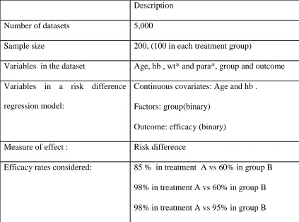
3.1.1 Number of simulated datasets and sample sizes ... 70
3.2 Characteristics of the simulated dataset ... 71
3.2.1 Parameter values for simulation of covariates ... 71
3.3 Randomization and the complete (full) dataset ... 72
3.4 Simulation of a binary outcome variable ... 73
3.5 Investigating the Binomial regression model and alternative approaches for modeling efficacy (risk) differences... 73
3.6 Investigating the effects of proximity to boundary of prevalence levels and number of covariates on convergence of a binomial regression model ... 74
3.7 The effect of correlations between covariates on model non-convergence ... 74
x
3.9 The “COPY method” and the binomial regression model ... 75
3.10 The Assessment of convergence and bias of the COPY method ... 77
3.11 The assessment criteria for the COPY method ... 77
3.12 Cheung‟s modified OLS method ... 78
3.13 Comparison of methods of dealing with missing binary outcome data ... 79
3.13.1 The mechanisms for making data to be missing ... 79
3.13.2 Missing completely at random scenarios ... 79
3.13.2.1 Missing at random scenarios ... 80
3.13.3 Rationale for choice of the efficacy rates... 81
3.13.4 Missing not at random scenarios ... 82
3.13.5 Model fitting ... 83
3.13.6 Assessment criteria ... 86
3.13.7 Software for simulations and analyses ... 86
CHAPTER 4 : Alternative approaches to fitting binomial regression model ... 87
4.1 Chapter structure ... 87
4.2 Binomial regression model ... 87
4.2.1 Factors associated with the failure of a risk difference binomial regression model ... 88
xi
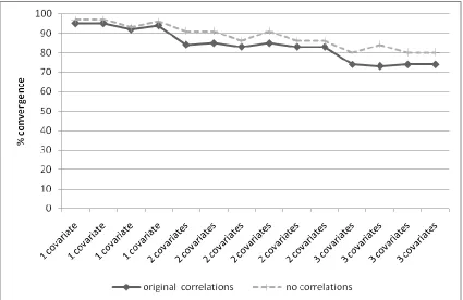
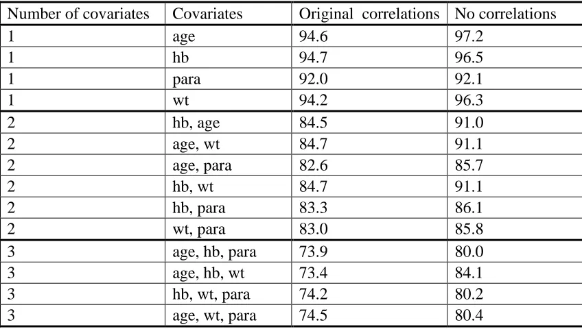
4.2.3 The effect of correlations between covariates on model non-convergence ... 92
4.3 The “copy method” and the binomial regression model ... 95
4.4 Aims of the copy method assessment ... 97
4.4.1 Methodology for data simulations for the copy method assessment ... 97
4.4.2 The assessment criteria ... 98
4.4.3 Copy method for a single original data set ... 98
4.4.4 Bias and convergence rate trends for the COPY method simulations ... 100
4.4.4.1Efficacy rates 85% vs. 60% ... 100
4.4.5 Copy method - bias and % convergence trends (95% vs. 90% efficacy rates) .... ... 103
4.4.6 Copy method - bias and % convergence trends (98% vs. 95% efficacy rates) .... ... 107
4.4.7 Cheung‟s Modified Ordinary Least Squares (OLS) method ... 110
4.4.8 Conclusion ... 112
CHAPTER 5 : An evaluation of methods for handling missing binary outcome values using imputation modeling ... 116
5.1 Mathematical approaches for imputing binary outcomes ... 116
5.2 Results for missing data simulations with binary imputed outcomes... 117
5.2.1 Missing At Random (MAR) scenarios... 118
xii
5.2.1.2 Efficacy rates 98% vs. 60% ... 121
5.2.1.3 Efficacy rates 98% vs. 95% ... 124
5.2.1.4 Imputing MAR binary outcomes with binary estimates - summary ... 127
5.2.2 Missing Completely At Random (MCAR) scenarios ... 128
5.2.2.1 Efficacy rates 85% vs. 60% ... 129
5.2.2.2 Efficacy rates 98% vs. 60% ... 131
5.2.2.3 Efficacy rates 98% vs. 95% efficacy ... 134
5.2.2.4 Imputing MCAR binary outcomes with binary estimates - summary .... 136
5.2.3 Missing Not At Random (MNAR) scenarios ... 137
5.2.3.1 Efficacy rates 85% vs. 60% ... 138
5.2.3.2 Efficacy rates 98% vs. 60% ... 140
5.2.3.3 Efficacy rates 98% vs. 95% ... 142
5.2.3.4 Imputing MNAR binary outcomes with binary estimates - summary .... 144
5.3 Results for missing data simulations with continuous imputed outcomes . 145 5.3.1 Missing At Random (MAR) scenarios... 146
5.3.1.1 Efficacy rates 85% vs. 60% ... 146
5.3.1.2 Efficacy rates 98% vs. 60% ... 150
5.3.1.3 Efficacy rates 98% vs. 95% ... 153
xiii
5.3.2.1 Efficacy rates 85% vs. 60% ... 159
5.3.2.2 Efficacy rates 98% vs. 60% ... 162
5.3.2.3 Efficacy rates 98% vs. 95% ... 165
5.3.2.4 Imputing MCAR continuous outcomes with binary estimates - summary 168 5.3.2.5 Missing Not At Random (MNAR) scenarios ... 169
5.3.3.1 Efficacy rates 85% vs. 60% ... 169
5.3.3.2 Efficacy rates 98% vs. 60% ... 172
5.3.3.3 Efficacy rates 98% vs. 95% ... 175
5.3.3.4 Imputing MNAR binary outcomes with continuous estimates - summary ... ... 177
5.3.3.5 Mathematical explanation of bias findings in the MNAR situation ... 178
CHAPTER 6 : Discussion and conclusions ... 186
6.1 The Binomial regression model, Copy method and Cheung‟s OLS method . 186 6.2 Comparison of methods of handling missing data ... 191
6.2.1 Imputing MAR binary outcomes ... 191
6.2.2 Imputing MCAR binary outcomes ... 196
xiv
6.4 The effect of missing values and the validity of the missing data simulation
findings ... 204
6.4.1 Study design ... 204
6.4.2 Outcome measure ... 205
6.4.3 Efficacy levels ... 206
6.4.4 Missingness, missingness levels and missingness mechanisms ... 206
6.5 Bias towards the null observed when wrong models are used (MAR and MCAR) ... 207
6.6 Perfect prediction in MI procedures ... 207
6.7 Bias towards the null observed when wrong models are used (MAR and MCAR) ... 209
6.8 Perfect prediction in MI procedures ... 210
6.9 Practical implications ... 211
6.9.1 Suggestions for further research ... 214
6.10 Summary conclusion and recommendations ... 216
References... 219
Appendices ... 226
Stata programs ... 226
Appendix: A1 stata commands for generating MCAR data ... 226
xv
xvi
List of tables
xvii
xviii
xix
xx
List of figures
xxi
Acronyms/Abbreviations
ACPR Adequate Clinical and Parasitological Response
AQ Amodiaquine
ART Artesunate
CC Complete Case analysis
CI Confidence interval
CQ Choloroquine
DR-IPW Doubly Robust Inverse Probability Weighting
EC Extreme case
GEE Generalized estimating equations
Hb haemoglobin
HR Hazard ratio
IPW Inverse Probability Weighting
ITT Intention- to- treat
LL Lower limit of a confidence interval
LOCF Last Observation Carried Forward
MAR Missing at Random
MCAR Missing Completely at Random
MCMC Markov Chain Monte Carlo
MI Multiple Imputation
MICE Multiple Imputation using Chained quations
MLE maximum Likelihood estimation
MNAR Missing Not at Random
xxii
OLS Ordinary Least Squares
OR Odds ratio
Para Parasitaemia
PCR Polymerase chain reaction
RCT Randomized controlled Trials
RD Risk difference
RR Risk ratio
SE Standard Error
SP Sulfadoxine Pyrimethamine
UL Upper Limit of a confidence interval
xxiii
Glossary/Definitions
Convergence Failure by software to provide output or (valid out output)
Covariate Continuous variable
Efficacy Proportion of participants with treatment success under controlled conditions
expressed as a percentage
Factor Categorical variable
Missingness Data being missing
Recrudescence Retain parasite genotype before and post treatment
Reinfections New parasite genotype infection after treatment
xxiv
Abstract
xxv
1
Chapter 1
: Missing binary outcome data in randomized controlled
trials
1.1 Background and motivation
2
The presence of missing data often complicates analyses and the strength of an RCT design may be compromised. Missing outcome data may lead to increased uncertainty over estimates of treatment effect and biased estimates if not properly dealt with in statistical analyses (Higgins et al. 2008).
3
the fact that the existing methods are only valid in specific missing data scenarios. Even the well known principled methods such as the MI methods (methods that fill in the missing observations with randomly generated plausible values based on other observed values) are biased in some situations and are not better than CC analysis in other settings (Allison 2001, White and Carlin 2010). The choice of the methods of handling missing data depends on the pattern of missing data as well as the mechanism that leads to the data being missing (Ibrahim and Molenberghs 2009). The patterns of missing data and missing data mechanisms are detailed in Chapter 2. In summary, the methods for handling missing outcome data are well developed for RCTs but are rarely applied in practice (Ibrahim and Molenberghs 2009) and the challenge is on the method choice that is most appropriate for a particular effect measure and missing data scenario since universally robust methods for handling missing data do not exist.
In RCTs, the intervention effect for binary outcomes is often measured using relative risks (RR), odds ratios (OR) or risk differences (RD) (Magder 2003). In recent years an RD has become a widely reported measure of effect in RCTs especially for malaria studies. Examples of trials that report a risk difference include: (Bell et al. 2008, Arinaitwe et al. 2009). Of note, an RD model sometimes fails to converge in software (Cheung 2007).
4
Considering that existing methods are not robust in all missing data scenarios, it is always important to perform simulation studies to compare the performance of different methods of dealing with missing data in order to identify the methods that are the most appropriate for a particular scenario.
Simulation studies have examined methods of handling missing binary outcome data where the summary measure of interest is an OR, for example: (Machekano et al. 2008, White and Carlin 2010, Groenwold et al. 2011). However, little is known on how the missing data methods perform when the outcome of interest is an RD rather than an OR. Clearly there is a gap in our knowledge of the most appropriate methods of handling missing outcome data when estimating the RD from an RCT.
5
used method to estimate an RD in the presence of missing outcome data in RCTs. It is important, therefore, to compare the performance of complete case analysis and multiple imputation approach in terms of bias and efficiency, for modeling an RD in the presence of missing outcome data in an RCT setting using simulations over a range of efficacy and missing outcome data scenarios.
Fitting a risk difference model uses the binomial regression model with an identity link function as the standard. However, this analysis approach is susceptible to model fail in software. The Copy method and Cheung‟s OLS method were potentially identified to be used in cases where the binomial regression model fails.
1.2 The “COPY method” and the binomial regression model
6
Mathematically, the copy method calculates MLEs using a log-binomial model on an expanded version of the data set that contains K-1 copies of the original dataset plus one copy of the original dataset in which the values of the binary outcome variable are reversed (the 1‟s (successes) are all changed to 0‟s (fails) and the 0‟s (fails) are all changed to 1‟s (successes)). When modeling a risk ratio using a log-binomial regression model, if the total number of dataset copies, K, is finite, the iterative estimation solution moves away from the parameter space and is an MLE for the “copied” dataset (Petersen and Deddens 2009).
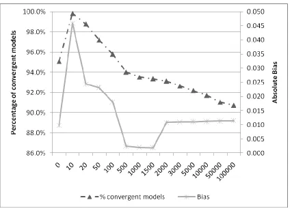
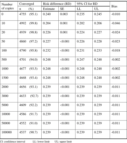
As K gets increases, the MLE estimate obtained from the “copied” dataset with a log-binomial model approaches the MLE estimate for the original dataset (i.e. is asymptotic) (Deddens and Petersen 2008, Petersen and Deddens 2008, Petersen and Deddens 2009). Petersen and Deddens (2008, 2009) recommend that K should be at least 100 (although in their paper they used a value of K = 1,000).
7
1.3 Cheung’s modified OLS method
Cheung (2007) proposed a variation of the Ordinary Least Squares estimation methodology to address the address the problem of non-convergence when modeling risk difference. The method uses a modified least-squares regression approach with a Huber-White robust standard error (Cheung 2007).
Simulation studies were performed to investigate the suitability of this method for modeling risk differences, in terms of both convergence and bias as an alternative to the binomial regression.
1.4Description of the motivating malaria efficacy clinical trial data
1.4.1 Study design
This research was motivated by a malaria efficacy study that was conducted in Malawi between 2003 and 2005 in children aged 1 to 5 years. The methods and the findings of this study are detailed in Bell et al (2008) but a brief summary of its rationale, design and findings follow:
8
(SP was the standard first line treatment for uncomplicated falciparum malaria in Malawi during the time when the study was conducted). The study was conducted in response to accumulating evidence indicating that SP was developing some resistance and because the WHO was recommending the use of combination therapies (especially the artemisinin combination therapies (ACTs)).
The study was done in Malawi and was based at the Chileka Health Centre. Chileka is a rural area in southern Malawi that has perennial malaria transmission that peaks during the rainy season. The rainy season in this area is between October and May, with the heaviest rains occurring somewhere around December to April.
All children in the study area aged between 1 and 5 years were screened for uncomplicated falciparum malaria. Children were recruited into the RCT if their weight was greater than or equal to 6 kg, if they had an axillary temperature of greater than or equal to 37.50C, if they had not been treated with an antimalarial drug or cotrimoxazole in the previous 4 weeks, and if they had a plasmodium falciparum parasite density of between 2000 and 200,000 parasites/ml – but were excluded from recruitment if they had any signs of severe malaria.
9
Measurements were taken from each recruited child on days 0, 1, 2, 3, 7, 14, 28 and 42 and on any other unscheduled day if they were sick during follow up. The clinical outcomes were assessed according to the 2003 WHO efficacy protocol (World Health Organization 2003). Children were withdrawn from the study if they missed a follow up visit detailed above, if they (or their guardian/carer) withdrew consent or if they took treatment that was considered to be a protocol violation/deviation.
1.4.2 Sample size and statistical methods
The study was designed to have 90% power to detect the following difference in the proportion of children with an „„adequate clinical and parasitological response‟‟ (ACPR) efficacy rate at the conventional 5% significance (alpha) level: 80% response in the SP plus placebo arm vs. 95% in at least one of the combination therapies. The literature available at the time the study was being designed indicated that SP was developing high resistance, so the efficacy of this treatment arm was anticipated to be 80% or lower. It was planned that each of the combination therapies would be compared in turn with the SP plus placebo group.
It was estimated that 85 children would be required in each treatment arm (total 340 children) to detect the desired combination treatment effect size. To allow for a loss to follow-up rate of up to 15%, the actual sample size was set at 100 children per treatment arm (total 400 children).
10
whether each participating child had a treatment failure or treatment success. Children were said to have had a treatment success if they had no fever and no parasaitaemia, otherwise they were said to have had a treatment failure.
The primary analysis of the primary endpoint was conducted using the intention to treat (ITT) principle whereby all children recruited into the trial were included in the analyses according to the group that they were randomized to. This was followed by a secondary analysis conducted using a per protocol analysis strategy (as a form of sensitivity analysis).
Almost all values were available for the baseline variables because these formed part of the inclusion or exclusion criteria. However, there were some children with missing outcomes due to a number of reasons, including: lost to follow-up, withdrawal of consent, withdrawn from study because of a protocol violation or deviation before the day 28 outcome was assessed. A few children had mixed plasmodium falciparum malaria genotypes post treatment. In many children for whom parasitaemia was detected during follow up, PCR was used to determine whether treatment was a success or not; however the outcome remained indeterminate for some children even after performing PCR.
11
second analysis irrespective of which treatment arm they had been allocated to. In the per-protocol (PP) analysis, all children with missing outcomes were excluded from the analytical process (again irrespective of which treatment arm they had been allocated to) - a method that is commonly referred to as “complete case analysis”. In order to improve accuracy, the PP analyses were done using polymerase chain reaction (PCR) corrected data to distinguish recrudescences from reinfections. When PCR results showed that a post-treatment parasitaemia genotype was a reinfection, the outcome was classified as a treatment success to the original parasitaemia genotype. If PCR result was indeterminate, the child was assigned a missing outcome value and was excluded from the per protocol analysis.
All data analyses were performed using the Stata for Windows software (version SE/8; statacorp; College Station, Texas 77845 USA). The outcome statistic chosen to indicate effect size was the risk (efficacy) difference between each intervention group and the control arm. Binomial regression models were fitted to the data and used to estimate the relevant risk differences (along with their corresponding 95%confidence intervals).
1.4.3 Missing outcomes
12
consent. The proportions of children with missing outcomes were similar across the treatment groups. Only negligible missing levels were observed in the covariates.
1.4.4 Results for the primary outcome of the historical data: efficacy of antimalarials
The efficacy rates were very high in all of the intervention arms. The AQ plus SP had an efficacy rate that was as high as 97%, 95% CI (93%, 99%) by day 28. The efficacy rate was close to the boundary value of 100%. Using the ITT analysis strategy in which the missing outcomes were assigned success values, the day 28 ACPR rate was lowest in the SP plus placebo group, which had an efficacy rate of 25%, 95% CI (18%, 34%), much lower than that anticipated (80%). The AQ+SP group had an ACPR rate of 97%; this was significantly higher than for the CQ+SP and ART+SP groups which had efficacies of 81%, 95% CI (73%, 88%) and 70%, 95% CI (61%, 78%) respectively (thus proving that in malaria treatment studies, efficacies close to the boundaries are just as possible as efficacy levels that are away from the boundary). There was no significant difference between the CQ+SP and ART+SP groups.
1.4.5 Motivation for designing simulation studies of missing data methods
13
From the literature on similar studies, we noted that authors tended to adopt a method of handling missing data arbitrarily without justification. Most commonly, methods were selected adhoc and usually involved extreme case (EC) analyses and complete case (CC) analyses. The CC analysis simply excludes any cases with missing outcome data while EC analysis simply replaces missing outcomes either all as successes or all as failures. Both of these methods are prone to bias especially when the levels of missing data are high. Statistical power may also be reduced in the case of complete case analysis.
In the absence of a clear guidance we were tempted to just choose the missing data methods that were being commonly used and to adopt the adhoc methods of complete case analysis for the per protocol analyses and extreme case analysis for the intention to treat strategy. We did not have any clear basis for the choice of these methods apart from being consistent with other researchers who had reported on the same subject area.
14
We were aware that the efficacy rates in the Bell et al study were very variable- some were very close to the 100% boundary while others were some distance away from the boundary – which could also complicate the analyses. For example, efficacies rates of 25%, 70%, 81% and 97% were observed in the “SP plus placebo”, “ART plus SP”, “CQ plus SP” and “AQ plus SP” treatment arms respectively. This provided a rationale for the choice of efficacy levels to be considered in a simulation study; efficacy levels were chosen in such a way that they covered the whole of the expected efficacy spectrum – some of the efficacy levels were chosen to be close to boundary values (in this context, close to 100%) while others were chosen to be away from the boundaries.
15
In most comparative studies, adjusted estimates of treatment effect are of interest, both to identify factors that are independently associated with the treatment effect size and to ensure that the effect size estimate presented is a true indication of the effect of the treatment of interest alone. However, risk difference modeling using the standard binomial regression model is susceptible to model failure (model convergence problems and estimate bias) when adjusting for other variables. This phenomenon provided additional motivation to examine factors that may be associated with the model failure and also to perform simulation studies to identify alternative methods that can be used when the standard binomial regression model fails to provide an adjusted estimate of effect size.
16
1.5 Aims of the project
1.5.1 Main objectives of the study
The primary objective of this research is to use computer simulation techniques to compare the performance, in terms of bias and efficiency, of the MI method and CC analysis approach for handling missing binary outcome data when modeling a risk difference in the presence of missing outcome data. The comparisons are performed over a variety of efficacy and missing binary outcome data scenarios, focusing on a randomized controlled trial design. Furthermore, this study identifies the factors that may lead to the convergence problems in software when estimating an adjusted risk difference.
1.5.2 Specific objectives
1. To compare the performance of the multiple imputation (MI) method and complete case (CC) analysis when estimating a risk difference from a randomized controlled design with the following missing data mechanisms:
a. missing at random(MAR);
b. missing completely at random(MCAR); c. missing not at random (MNAR).
2. To assess how the closeness of the efficacy to a boundary value (i.e. to 0% or 100%) impacts the estimates from CC and MI in terms of bias and efficacy by considering the following efficacy scenarios:
17
b. the efficacy rate in one treatment arm is close to a boundary value while in the other arm it is away from a boundary value;
c. the efficacy rates are close to a boundary value in both treatment arms. 3. To investigate the impact of the following factors on non-convergence of a
binomial model that estimates a risk difference in Stata statistical software package:
a. one or both efficacy rates close to a boundary value; b. the number of covariates in a model;
c. the correlations between covariates.
4. To assess the appropriateness of the binomial model, the COPY method of the binomial model and Cheung‟s OLS method in terms of convergence and bias.
1.6 Significance of the study
18
be used in the MI process that are most likely to produce unbiased estimates of the effect difference and minimize the risk of model failure.
1.7 Structure of the thesis
19
Chapter 2
: Literature review
This Chapter describes the common measures of effect for a binary outcome variable in RCTs and reviews missing data theory in this situation, focusing on common approaches to handling missing binary outcome observations. Both unprincipled and principled statistical methods are reviewed, and the strengths and weaknesses of each are discussed. This Chapter is structured as follows: firstly, common measures of effect when modeling a binary outcome data in RTCs are described; missing data theory in general is then reviewed; finally, common approaches to handling missing binary outcome observations are discussed.
2.1. Common measures of effect for binary outcome data in RCTs
The measures of effect in RCTs where the outcome of interest is binary include: odds ratios (OR), relative risk/risk (rate, hazard) ratios (RR), risk (rate, hazard) differences (RD) and number needed to treat (NNT). However, the most commonly used measures are: OR, RR and RDs; there are many examples of these measures reported in the research literature for example: (Faucett et al. 2002, Brasseur et al. 2007, Bell et al. 2008, Borrmann et al. 2008, Crompton et al. 2008, Faucher et al. 2009, Gesase et al. 2009, Chasela et al. 2010, French et al. 2010).
20
computational difficulties such that regression models of binary data could only be done on odds ratios and not on risk or rate ratios, even though the theory had been well developed (Cox and Snell 1970). In fact the Cox proportional hazards regression model (Cox 1972) was the first method adopted widely to model rate ratios before Poisson and negative regression models appeared in the widely used statistical computer packages. The Cox proportional hazards regression model estimates risk ratios by setting the follow-up time to 1 (Cummings 2009b).
However, there has been a lot of debate as to which of a RR or an OR is the most appropriate statistic to use (Barros and Hirakata 2003); this debate has been extended to also include RDs. It has been argued that the OR has been in wide use because it is computationally less challenging than the alternatives RR and RDs (Wacholder 1986). When analyzing case-control studies, of course, the OR is the only appropriate statistic to use to compare risks; the relative risk is mathematically invalid because the selection of study participants is based on outcome and not exposure (Miettinen and Cook 1981).
21
prevalence of the outcome measure is common, can easily yield incorrect inferences of treatment effect ( Davies et al. 1998, Case et al. 2002, McNutt et al. 2003, Page and Attia 2003, Cheung 2007).
An OR is routinely chosen as a measure of effect often based on mathematical convenience without consideration of whether the results are interpretable (Walter 2000). The relative risk, on the other hand, occupies a very special role as a measure of effect for binary outcome in cohort studies, in which exposure usually precedes outcome and it is generally befitting to use an RR as a measure of effect. For some time now, many researchers have been recommending a systematic use of the RR rather than the OR whenever appropriate (Axelson et al. 1994, Davies et al. 1998, Grimes and Schulz 2008, Cummings 2009a). RDs and RRs are sometimes more biologically plausible than ORs which may give them an advantage when describing a risk (Walter 2000).
22
2.2 Risk difference modeling and alternative methods 2.2.1 Odds ratios and risk ratios
In comparative studies where the outcome of interest is binary, odds ratios or risk ratios are most commonly used to model intervention effect size.
The odds ratio is the only valid summary statistic in case control studies where the selection of study participants (cases and controls) is based on the outcome rather than the exposure - in this case a risk ratio cannot be computed directly. More precisely: the odds ratio compares the relative odds of a (binary) outcome between treatment groups; it is also a commonly used measure of strength of association between outcome and exposure in case-control studies. Odds ratios can most easily be obtained from a logistic regression model.
23
The odds ratio is still used widely as the preferred measure of effect even in situations where a risk ratio is probably more appropriate. There are several reasons for this:
The odds ratio has important computational advantages over both the risk difference and the risk ratio when adjusting for covariates (Wacholder 1986).
The odds ratio does not have the convergence problems encountered in many software packages when attempting to estimate and/or manipulate risk ratios and risk differences.
Most reports of cohort studies in the past have used odds ratios, so using this statistic for new cohort studies provides a more ready comparison with findings from previous studies.
24
from the value of the odds ratio estimate as this error is a function of the underlying probabilities rather than of the odds ratio itself.
The risk ratio also has some limitations, including potentially important interpretation problems. For example, the risk ratio for the outcome Y = 0 is not the inverse of the risk ratio for the outcome Y= 1 (Blizzard and Hosmer 2006). This means that when risk ratios are used in some RTCs and equivalence studies, evidence of equivalence in the failure rate does not necessarily come with evidence of equivalence in the success rate (Cheung 2007). This dilemma considerably limits the use of the risk ratio in some situations (Cheung 2007).
2.2.2 Risk difference and rationale for its choice
The risk difference is an alternative statistic for presenting effect size estimates derived from binary outcome data, and seems to be the most appropriate method in situations where efficacy is high in both treatment groups.
25
were 4 times (and statistically significantly) more likely to fail than those in the intervention group, with the 95% confidence interval indicating that the true risk ratio lies between 2 and 8. On the other hand, using the odds ratios as an alternative for this data gives OR=4.1 (95% CI 2.0 : 9.3; p<0.001). The interpretation of this is that the odds of treatment failure in the control group is just fractionally over 4 times (and statistically significantly) greater than the odds of treatment failure in the intervention group and that we can be 95% confident that the true population odds ratio lies somewhere between 2.0 and 9.0. Clearly, both of these statistics considerably exaggerate the real (i.e. clinically important) difference in the relative effects of the two treatments.
26
As studies are increasingly being analysed using risk differences, it is becoming appealing for new studies to be analysed in a similar manner so that the outcome measures from different studies can be combined in a meta-analysis /systematic review. Risk difference estimation is preferred by many researchers because it is easier to interpret than the alternative odds ratio. A risk difference is symmetric so evidence of equivalence in failure rate is mathematically equivalent to evidence of equivalence in success rate (Cheung 2007); risk ratios, on the other hand, are not symmetric. These trends were the primary motivating factor for consider a risk difference model in the simulations presented in this dissertation.
The binomial regression model with an identity link function is used to fit a risk difference model. However, fitting a risk difference model often encounters the problem that the binomial regression model fails to converge (Cheung 2007).
2.2.3 Mathematical principles underlying analytical approaches in risk difference models
27
Estimation of probabilities a logistic regression model (Odds ratios)
Consider the following generalized linear model (GLM) again: Replace μ with π to estimate probabilities:
If the aim of the analysis is to estimate odds ratios, a logit link function is used in the GLM and the GLM becomes:
This will result in probability estimates that lie between 0 and 1. This is the reason why logistic regression model is likely to converge and provide sensible estimates from the equation 2.6 below:
Estimation of probabilities from risk difference model (binomial regression with identity link)
Consider the following generalized linear model (GLM)
) 1 . 2 ...( ... ... ... ... ... )
( 1X1 kXk
g
k kX
X
g() 1 1
) 2 . 2 ...( ... ... ... ... ... )
( 1X1 kXk
g
) 3 . 2 ( ... ... ... ... ... 1
ln 1X1 kXk
) 6 . 2 ..( ... ... ... ... ... ... ... 1
1X kXk ) 4 . 2 ..( ... ... ... ... ... ) ... exp( 1 ) exp( 1 1 1 1 k k k k X X X X ) 5 . 2 ....( ... ... ... ... ... )) ... ( exp( 1 1 1
28
where g(u) is a link function that identifies a function of the mean that is a linear function of the covariates and is a set of k explanatory variables.
When the outcome is binary, u becomes π (the proportion of participants with an outcome of interest); in other words, π is the probability of observing a specific category of the binary outcome. Thus, the GLM can be re-written as in equation 2.2:
If the aim of the analysis is to estimate risk differences, an identity link function is used in the GLM which reduces to:
From the equation above, it should be noted that the estimate of π as a linear function of explanatory variables can easily yield estimates of probabilities that are outside the valid range 0 to 1. This is so because the expression is unbounded and can yield values that range from - to +. But since a binomial model is constrained to estimate probabilities that are between 0 and 1, the estimates of probabilities that are outside this range may result in computer software not providing results.
k
X X1
k kX
X
g()1 1
) 7 . 2 ...( ... ... ... ... ... ... 1
1X kXk k kX X
29
Now if we consider (2.7)
and suppose X1 is a binary exposure (0 or 1) that may denote the treatment/ intervention that an individual is assigned to. Then the estimate of the adjusted risk difference becomes:
So the estimate of the risk difference is just and this does not have boundary constraints as is the case with the estimation of probabilities. This suggests that if interest is in estimating the risk difference rather than the individual risks (probabilities) themselves, estimates of the risk difference based on the above linear model would be valid. This is also demonstrated by Cheung (2008), when he established that Ordinary Least Squares estimation methods with Huber White standard errors are valid for the estimation of risk differences. This method also avoids the non-convergence problems that can be experienced when using the binomial regression model with an identity link function because the core function of this binomial regression model is the estimation of probabilities. It has already been shown above that such estimation of probabilities based on the standard binomial regression model may result in probabilities that are outside 0 and 1 because the linear function of the covariates is unbounded. The Cheung‟s method for modelling risk difference is described in detail in section 3.13 of this dissertation.
k kX
X
1 1
) 9 . 2 ....( )}... ˆ ... 0 ˆ ˆ ( ) ˆ 1 ˆ ˆ
{( 1 kXk 1 kXk
RD
) 8 . 2 ...( ... ... ... ... ... ... ... ... ˆ
ˆ1 0
30
2.3 Theory of Missing Data
In this section missing data theory is reviewed.
2.3.3 Missing Data Mechanisms
Missing data is a common problem in many research disciplines. The process that results in missing data is technically known as the missing data mechanism (Rubin 1976, Schafer 1997, Little 2002). When handling missing data in a statistical analysis, the choice of missing data methods hugely depends on the missing data mechanism (Schafer 1997). In order to choose an appropriate statistical methodology, therefore, it is imperative for the analyst to have an idea or some plausible assumption of the missing data mechanism present in the data. In his theory, Rubin (1976) developed a useful taxonomy for describing the assumptions regarding the missing data mechanisms which provides an important guide to researchers on how to deal with missing data in analyses. The missing data theory regards the missingness of data as a probabilistic event. The commonly made assumptions about the distribution of missingness and the missing data taxonomy are based on Rubin (1976) are reviewed below.
2.3.4 The Distribution of Missingness
31
Consider a longitudinal study into which n subjects are enrolled and followed up over time such that measurements are taken at baseline and then at specified times during the follow up (t assessment times in total).
Let Yij and Xij represent the outcome and a covariate data respectively for study
participant i (i = 1,2,… , n) measured at time j (j = 1,2,…, t).
In general Yij and Xijdenote a complete dataset for a longitudinal study where data is collected repeatedly over time. In a typical RCT study, for reasons that may be beyond the investigators‟ control, not all of the Yij and Xij will be observable for all study participants no matter how rigorous the researchers may be (i.e. there will be missing data, and these may occur in the outcome variable as well as in the covariates). The reasons for missing data are usually difficult to precisely determine in practice.
Let Yi
Yi1,...Yit
Tbe a complete vector of outcomes for individual i taken at timest j1,2,....,
32
Thus Yi can be re-written as
( ), i(miss)
obsi
i Y Y
Y , where (obs)
i
Y denotes the observed data and (miss)
i
Y denotes the missing outcomes which should have been observed for individual i.
Further, let Di
Di1,...Dit
T be a vector that indicates missingness such that if
1 ij i(miss)
ij Y Y
D and Dij 0 ifYijYi(obs) where є means „belongs to‟
Since, as has been previously mentioned, it is often difficult to precisely establish the source of missing data in a dataset, the probability distribution function of the missing data indicator variables Di given the fully observed data Yi, is often used as the best
statistical tool to explain the process that is creating missing data in a dataset and is denoted as f(Di |Yi) (Schafer and Graham 2002).
In this thesis, a special case where missingness is only in the outcome and where the outcome is measured only once at the end of the study is considered. Furthermore, the baseline variables are collected at the beginning of the study only. This is a common design in malaria efficacy RCTs. Now considering this special case, the notations and descriptions are presented as follows:
Let Yi and Xirepresent the outcome and a covariate respectively for study participant i (i
33
Let Ybe a complete vector of outcomes for all individuals in the study. This data can be partitioned into those whose outcomes have been observed and those whose outcomes are missing.
Thus, Y can be presented asY
Y(obs),Y(miss)
, where Y(obs) denotes the observed binary outcome data and Y(miss)denotes the missing binary outcomes which should have been observed.In this special case, let D be a vector that indicates missingness such that if
1 Yi Y(miss)
D and D0 ifYiY(obs) where є means „belongs to‟.
The standard nomenclature for missing data mechanisms (Rubin D.B 1976) classifies missing data mechanisms as (i) missing at random (MAR), (ii) missing completely at random (MCAR), or (iii) missing not at random (MNAR).
2.3.5 Taxonomy for missing data mechanisms
34
2.3.6 Missing At Random (MAR)
In longitudinal studies where data is repeatedly collected overtime, the outcome data are said to be missing at random (MAR) if the probability of being missing depends on the observed outcome values and the covariates, but is independent of the specific missing outcome values that should have been observed in principle. In mathematical terms this is expressed as follows:
) ( | , , ) for all ,
, , |
(Di Yi Xi f Di Yi(obs) Xi Yi(miss)
f ………..……(2.11)
where
denotes a set of unknown parameters governing the missing data indicators; Yi ,Xi and Di are the complete outcome data, the covariates and missing data vectorsrespectively.
Example
35
cases for which Hb is observed as it is among the cases for which Hb level is missing; however, the distribution of Hb values for participants with observed age = 11 may be different from the distribution of HB values for those with observed age = 10 years. The same applies for participants with observed age = 12 years, 13 years… etc. That is, the missing Hb values should be regarded as a random sample of all the Hb values within the observed age subgroups.
The practical challenge with the MAR mechanism is that it is often difficult to confirm that the probability of data on Y being missing entirely as a function of observed data (Little 2002). However, MAR is often plausible in practice (Schafer and Graham 2002, Kenward and Carpenter 2007).
2.3.7 Missing Completely At Random (MCAR)
The outcome data are said to be missing completely at random (MCAR) if the probability of being missing does not depend on either the value of the outcome Y or the value of the covariate.
Mathematically this is expressed as follows:
) ( | ) for all , ,
, , |
(Di Yi Xi f Di Yi Xi
36
In fact this is a special case of MAR in which the probability that data are missing is independent of both the specific missing values that in principle should have been observed and the values of the observed data (Schafer 1997, Schafer and Graham 2002).
Example
Revisiting the example above, MCAR implies that the missing Hb values are neither related to age nor to the other Hb values (whether observed or not). Thus, with MCAR, the component of the data with missing Hb values is a random subset of the complete original sample of Hb values – and equally, by definition, the observed sample is also a random sample of the original complete sample. In fact, MCAR implies that the missing values are a random sample of all values of the population from which the study sample came (Rubin 1976). A typical practical example of MCAR would be a test tube containing a laboratory sample being accidentally broken before the sample has been processed or the sample become contaminated or non-viable because of an electricity failure to the storage facility.
2.3.8 Missing Not At Random (MNAR)
The outcome data are said to be missing not at random (MNAR) if the probability that the outcome data are missing depends on both the observed outcome values and the unobserved outcome values. In mathematical terms this is expressed as follows:
) ( | , , , ) for all , ,
, X , |
(Di Yi i f D Y(obs)Y(miss) Xi Yi Xi
37 Example
Consider an HIV longitudinal study in which CD4 count is measured for each participant at each clinic visit during follow-ups. Suppose that some participants may drop out of the study before the study ends due to HIV related death. These “drop-outs” will have missing CD4 count at visits scheduled after they died; it is also likely that they will also have low CD4 counts as this is known to be related to HIV related death. In such cases, therefore, the missing CD4 counts will be correlated with the actual missing values (i.e. those with a low CD4 are more likely to die due to HIV related death than those with a high CD4, or more relevantly to the context of this dissertation, those with unobserved but a low CD4 count at a missing visit will be more likely to have a missing CD4 count value at the that visit because of the value of the CD4 itself which is low and therefore may be related to death from HIV related cause). This would be a typical example of MNAR.
38
2.3.9 Taxonomy for missing data mechanisms described for a special case of an outcome variable collected once at the end of the study
2.3.9.1Missing At Random (MAR)
Consider a special case where data is missing only in the binary outcome variable Y, the outcome data are said to be missing at random (MAR) if the probability of being missing depends on the observed covariates, but is independent of the specific missing outcome values that should have been observed in principle. In mathematical terms this is expressed as follows:
) | 1 ( Pr ) , | 1
Pr(D Y X D X ………
……….(2.14)
where Y , X are the complete outcome data, the covariates and D is a vector that indicates missingness such that D1 if Y is missing and D0 if Y is observed
Example
39
which efficacy is missing. Similarly, for study participants with observed age = 11 years, the chance of treatment success is the same among the cases for which efficacy is observed as it is among the cases for which efficacy is missing; however, the chance of treatment success for participants with observed age = 11 and are on placebo may be different from the chance of treatment success for those with observed age = 10 years and are on placebo. The same applies for participants with the specified observed ages above but who are on active treatment. This also applies to participants with observed age = 12 years, 13 years, …, etc conditional on their treatment status. That is, the missing efficacy should be regarded as a random sample of all the efficacy values within the observed age by treatment subgroups.
2.3.9.2Missing Completely At Random (MCAR)
The outcome data are said to be missing completely at random (MCAR) if the probability of being missing does not depend on either the value of the outcome Y or the value of the covariate.
Mathematically this is expressed as follows:
) 1 Pr( ) , | 1
Pr(D Y X D ………(2.15)
40 Example
Reconsider the example above, MCAR implies that the missing efficacy values are neither related to age, treatment on which someone is on nor to the efficacy itself (whether observed or not). Thus, with MCAR, the component of the data with missing efficacy is a random subset of the complete original sample of efficacy status – and equally, by definition, the observed sample is also a random sample of the original complete sample.
2.3.9.3Missing Not At Random (MNAR)
The outcome data are said to be missing not at random (MNAR) if the probability that the outcome data are missing depends on both the observed outcome values and the unobserved outcome values. In mathematical terms this is expressed as follows:
X) , Y , Y | 1 ( Pr ) X , | 1
Pr(D Y D obs mis ………(2.16)
2.3.10 Remarks on MAR, MCAR, and MNAR assumptions
There are important implication of the different missing data mechanisms: MAR, MCAR and MNAR (Rubin 1987, Allison 2001, Collins et al. 2001, Little 2002, Schafer and Graham 2002).
41
Y. When the data Y is fully observed, h(Y,) describes both the sampling distribution for Y and the likelihood function for. Thus, when the data is fully observed for Y, the fact that h(Y,)may be regarded as a likelihood function for allows the application of Maximum Likelihood (ML) methods to obtain valid estimates of (Schafer and Graham 2002).
The situation is different in the presence of missing data. It is only under the MCAR assumption that the distribution of the observed data only denoted as h(Y(obs),) can be regarded as both a correct sampling distribution of Y and a correct likelihood function for
producing valid ML estimates of. In the presence of the missing Y, the distribution )
, (Y(obs)
h is not a correct sampling distribution of Y under MAR assumption. However,
it is a correct likelihood function for under MAR (Rubin 1976, Schafer 1997, Little 2002, Schafer and Graham 2002). Thus when the data is MAR, the ML based estimation methods yield valid estimates of .
42 Example
Consider an RCT to determine the efficacy of ant-malaria therapy by day 28 from the time participants took their first dose. The day 28 outcome would be assessed on all participants if there were no losses to follow up. It may also be possible that due to cost implications, a researcher may decide to follow up fewer participants up to day 42 and day 63 as secondary endpoints. A researcher can decide to take a random sample of 80% from the original sample. This means that some participants (20%) will have missing day 42 and day 63. If all the 80% of the original sample that has been sampled for further follow up will be successfully followed up without losses to follow up, then those that will have missing day 42 and day 63 observations will be MCAR.
MAR is less restrictive than MCAR and is generally plausible in practice (Collins et al. 2001, Kenward and Carpenter 2007). MAR assumption plays a critical role in the process of handling missing data because valid inferences can be made without regard to the missing data mechanism (Rubin 1976, Little 2002, Schafer and Graham 2002, Carpenter et al. 2007, Kenward and Carpenter 2007).
2.3.11 Missing data patterns
43
data patterns. For the purposes of this thesis univariate pattern, monotone pattern and General pattern will be discussed.
2.3.11.1 Univariate missing data pattern
This is a data configuration such that data is fully observed for variables X1, X2,…, Xk
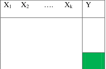
[image:68.612.102.272.506.617.2]but is missing for some participants for variable Y (Schafer and Graham 2002, van Buuren 2007, Enders 2010). This pattern may arise in randomized controlled trials where baseline variables are rigorously measured at baseline and form part of inclusion/exclusion criteria but may be missing for an outcome variable that is measured during follow-up. Figure 2.1 below gives a graphical presentation of a univariate pattern. In general this is not a common pattern in many study designs. Even in well designed randomized studies presence of some missing data in the baseline covariates is inevitable.
Figure 2.1: Illustration of a univariate missing data pattern based on (Schafer and Graham 2002, Enders 2010)
X1 X2 …. Xk Y
44
2.3.11.2 Monotone missing data pattern
This pattern usually occurs in studies where participants are followed over time. Consider data Y1, Y2, ..., Yk that are longitudinally collected at times t1, t2, t3,….., tk respectively.
Monotone pattern means that if data is missing for Yi then it will also be missing for
[image:69.612.254.397.303.476.2]Yi+1…..YK. This missing data pattern is illustrated in figure 2.2 below.
Figure 2.2: Illustration of a monotone missing data pattern based on (Schafer and Graham 2002, Enders 2010).
Y1 Y2 …… YK
(The shaded area represents the missing data.)
2.3.11.3 General missing data pattern
45
Figure 2.3: Illustration of a general missing data pattern (the shaded area represent missing data)
Y1 Y2 . . Yk
2.4 Common approaches for handling missing data
2.4.3 Unprincipled (adhoc) methods
The unprincipled statistical methods are methods for handling missing data which are not based on statistical models (Kenward and Carpenter 2007). In these methods the data are manipulated such that analyses proceed as if data was completely observed without paying attention to the process that is creating missing data (Kenward and Carpenter 2007). These methods often yield invalid inferences (Kenward and Carpenter 2007). Despite the existence of a variety of principled statistical methods of handling missing data, missing data is quite commonly handled using unprincipled methods.
46
2.4.4 Complete case analysis
47
randomized controlled trials (Altman 2009). The intention to treat principle requires that all subjects that were randomized in a study are included in the analysis according to their randomization.
2.4.5 Last observation carried forward (LOCF)
LOCF is also one of the commonest solution for analyzing continuous outcome data with some missing observations from randomized studies which are longitudinal in design (Altman 2009). Missing data for subjects that dropout in longitudinal studies are replaced by the last observed measurement taken before the participant dropped out of the study. This method greatly simplifies analyses but is highly prone to producing biased estimates (Streiner 2008, Altman 2009). It assumes that from the time the last observation was taken, the value would have remained the same over time. This is not plausible in many cases (Shapiro 2001, Streiner 2008, Altman 2009). Observations are usually variable within an individual over time. The main advantage of this approach in randomized studies is that it allows application of the Intention to treat principle. However it should be noted that although the method is compatible with ITT principle, the estimates may be biased, making the inferences difficult to generalize (Lee et al. 1991, Shapiro 2001, Streiner 2008, Marshall et al. 2009).
Example
48
and 28. Let the outcome of interest be adequate clinical and parasitological failure. A subject dropping out of the study after day 3 measurement and before day 7 will have the day 3 measurement as the last observation. The is participant has a higher chance of having treatment failure on day 3 because of pharmacokinetic reasons and it may be difficult to justify an assumption that the outcome of this particular participant would have remained the same up to day 28. Furthermore, if the dropout is in the placebo/control treatment group the resulting estimates of treatment effect may be biased in favour of the active treatment when LOCF approach is used (Streiner 2008). In longitudinal studies it is very unlikely that the last measurement would have remained the same up to the end of follow up because correlation between repeated measurements tend to decrease with increasing time separation (Diggle et al. 2002, Hedeker and Gibbons 2006).
2.4.6 Extreme case (EC) analysis
49
2.4.7 Single imputation methods
2.4.7.1Mean imputation
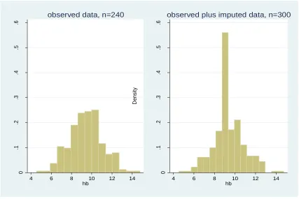
In the mean imputation each missing value is replaced by the marginal mean. The main problem with this approach is that it alters the shape of the distribution of the imputed variable (figure 2.4). This method produces biased parameter estimates of location and in addition, it does not account for uncertainty due to imputed values (Enders 2010). Of course the obvious advantage is that it results in complete data which can then be analysed by any standard method of analysis.
Example
50
Figure 2.4: Histograms of the observed data and the complete marginal mean imputed data 0 .1 .2 .3 .4 .5 .6 D e n si ty
4 6 8 10 12 14
hb
observed data, n=240
0 .1 .2 .3 .4 .5 .6 D e n si ty
4 6 8 10 12 14
hb
observed plus imputed data, n=300
2.4.7.2 Hot Deck imputation
[image:75.612.111.538.139.424.2]51
The obvious advantage of this method is that it results in complete data that can be analysed by any standard statistical method. In addition it is consistent with the intention to treat principle. It will always result in a plausible range of results (Andridge and Little 2010). However the method lacks theoretical basis (Andridge and Little 2010). Just like other single imputation methods, this method results in small standard errors due to the fact that uncertainty in the imputed values is not taken into account in the substantive analyses because the imputed values are treated as if they were actually observed.
2.4.7.3 Regression imputation - Buck’s method
This method was proposed by Bulk (1960). It obtains information for imputing missing values from other observed variables in the dataset (Buck 1960). It is also referred to as conditional mean imputation (Enders 2010). Let Y,X1,X2,...,Xpbe the p+1 variables in a dataset such that Y values are missing for some participants and the variables X1, . . .
,Xp are fully observed for all participants in the dataset. Firstly, the following regression
model is fitted to the observed data as follows:
p pX
X
Y 0 1 1.... ………(2.17)
The missing Y value for individual i is then imputed using estimates from the regression equation below:
pi p i
i X X
Yˆ ˆ0ˆ1 1 ....ˆ ………...(2.18)