A 1-parameter approach to links in a solid torus

doi: 10.2969/jmsj/06210167

A 1-parameter approach to links in a solid torus

By Thomas FIEDLERand Vitaliy KURLIN (Received Nov. 10, 2008)

Abstract. To an oriented link in a solid torus we associate a trace graph in a thickened torus in such a way that links are isotopic if and only if their trace graphs can be related by moves of finitely many standard types. The key ingredient is a study of codimension 2 singularities of link diagrams. For closed braids with a fixed number of strands, trace graphs can be recognized up to equivalence excluding one type of moves in polynomial time with respect to the braid length.

1. Introduction.

1.1. Motivation and summary.

The classical Reidemeister theorem says that plane diagrams represent isotopic links in 3-space if and only if they can be related by finitely many moves of 3 types corresponding to the codimension 1 singularities of links diagrams, namely a triple point , simple tangency and ordinary cusp .

We establish the higher order Reidemeister theorem considering a canonical 1-parameter family of links in a solid torus and studying codimension 2 singularities of resulting link diagrams. The 1-parameter family of link diagrams is encoded by a new combinatorial object, a trace graph in a thickened torus in such a way thattrace graphs determine families of isotopic links if and only if they can be related by a finite sequence of the11moves in Figure11, see Theorem 1.4. The conjugacy problem for braids is equivalent to the isotopy classification of closed braids in a solid torus. Braids areconjugateif and only if the trace graphs of their closures areequivalentthrough only tetrahedral moves and trihedral moves in Figure 11i, 11xi. Trace graphs of closed braids can be recognized up to isotopy in a thickened torus and trihedral moves in polynomial time with respect to the braid length, see Theorem 1.5. The method provides a new geometric approach to the conjugacy problem for braid groupsBn, which still has no efficient solution for n!5 strands, i.e. with a polynomial complexity in the braid length. Very promising steps towards a polynomial solution were made by Birman, Gebhardt,

2010Mathematics Subject Classification. Primary 57R45; Secondary 57M25, 53A04.

Key Words and Phrases. knot, braid, singularity, bifurcation diagram, trace graph, diagram surface, canonical loop, trihedral move, tetrahedral move.

#2010 The Mathematical Society of Japan J. Math. Soc. Japan

Vol. 62, No. 1 (2010) pp. 167–211

Gonza´lez-Meneses [3] and Ko, Lee [11]. A clear obstruction is that the number of different conjugacy classes of braids grows exponentially even in B3, see Murasugi [13].

Usually links are studied in terms of braids using the theorems of Alexander and Markov, see Birman [2]. The 1-parameter approach is a geometric alternative to the algebraic one: conjugacy of braids and Markov moves are replaced by a stronger notion of link isotopy and extreme tangency moves in Figure 11viii, respectively.

1.2. Basic definitions.

We work in theC1-smooth category. Fix Euclidean coordinatesx; y; zinR3. Denote byDxythe unit disk with centre at the origin of the horizontal planeXY.

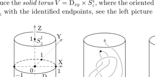
Introduce thesolid torusV ¼Dxy#S1z, where the oriented circleS1zis the segment

½%1;1&zwith the identified endpoints, see the left picture of Figure 1.

DEFINITION1.1. An embedding is a diffeomorphism onto its image. An

oriented link K'V is the image of an embedding f :Fjm¼1Sj1!V. An isotopy

between two oriented links K0 and K1 in V is a smooth map F :ðFmj¼1Sj1Þ #

½0;1&!V such that f0ðFmj¼1S1jÞ ¼K0, f1ðFmj¼1S1jÞ ¼K1 and the maps fr¼ Fð*; rÞ:Fm_j¼1S1

j !V are smooth embeddings for all r2½0;1&.

Mark n points p1;+ + +; pn2Dxy. A braid ! on n strands is the image of a

smooth embedding ofnsegments intoDxy# ½%1;1&z such that (see Figure 1)

, the strands of! are monotonic with respect toprz:!!Sz1;

, the lower and upper endpoints of!are Sðpi#f%1gÞ,

S

ðpi#f1gÞ,

respec-tively.

Braids are considered up to isotopy in the cylinder Dxy# ½%1;1&z, fixed on its

braid consists ofnvertical segmentsFn_i¼1ðpi# ½%1;1&zÞ. A braid!2Bn ispureif

the induced permutation!~2Snof its endpoints is trivial. Theclosedbraid!^'V

is obtained from!'Dxy# ½%1;1&zby identifying the bases fz¼ -1g.

The smoothness of a link K implies that the tangent vector f_ðsÞ never vanishes on K. The standard unknot is given by the trivial embedding S1z ! V ¼Dxy#Sz1. We introduce a new equivalence relation,strong isotopy, for links

in a solid torus. For closed braids, the usual isotopy through closed braids is strong.

DEFINITION1.2. Anextreme pairof a linkK'V is a pair of either 2 local maxima or 2 local minima of the projectionprz:K!Sz1 with the same z-coordinate. A smooth isotopyF :ðFmj¼1S1jÞ # ½0;1&!V of links is called strong

if all links in the family Kr¼Fð

Fm

j¼1S1j; rÞ 'V have no extreme pairs for r2½0;1&.

H. Morton proposed the trivial knot in the middle picture of Figure 1. The

Morton unknot is not strongly isotopic to the standard unknot S1

z. The arc

between the marked extrema is a long trefoil that can not be unknotted by strong isotopy since the marked extrema remain the highest and lowest critical points.

1.3. Trace graphs of links.

Links are usually represented by plane diagrams with double crossings. A classical approach to the classification of links is to use isotopy invariants, i.e. functions defined on plane diagrams and invariant under the Reidemeister moves. The Reidemeister moves in Figure 5 correspond to simplest singularities that can appear in diagrams of links under isotopy, e.g. Reidemeister move III describes the change of a diagram when a transversal triple intersection appears in the projection.

The analogue of a plane diagram in the 1-parameter approach is a 1-parameter family of diagrams obtained by rotating a link in V around S1

z. This is a

2-dimensional surface containing more information about the link than only one plane diagram. The link will be reconstructed up to smooth equivalence from the self-intersection of the surface, the trace graph. Denote by rott:V !V the rotationof the torusV aroundS1

z through an anglet2½0;2"Þ, see Figure 2. Heret

is the parameter on the time circle S1

t ¼R=2"Z of length 2". Let Axz be the

vertical annulus ½%1;1&x#Sz1 in the solid torus V. Define the thickened torus

DEFINITION1.3. The trace graphTGðKÞ 'T of a link K'V consists of the crossings of the diagramsprxzðrottðKÞÞover allt2S1t. Mark the intersection

points fromKTðDxy#f-1gÞ 'V and also mark each local extremum ofKwith

respect to prz:K!Sz1. If K has m components, in general position, the i-th

component decomposes into ni vertically monotonic arcs labelled by Aiq, q¼1;+ + +; ni. The 3 monotonic arcs in Figure 2 are numbered simply by 1, 2, 3.

Take a point p2TGðKÞ, which is a crossing of Aiq overAjs in the diagram

prxzðrottðKÞÞ for some t2St1. Associate to p the ordered label ðqisjÞ. Then the

edges of the graphTGðKÞare labelled. In the casem¼1we miss the indicesi; jof components ofKand label edges by ordered pairsðqsÞ, see Figure 3.

For each t2S1

t, watch the crossings of the diagram prxzðrottðKÞÞ 'Axz#

ftg, e.g. the initial diagramprxzðKÞ 'Axzat t¼0has 3 double crossings, which

evolve during the rotation ofK. Att¼"=4, the lowest crossing becomes a critical Figure 3. The trace graphTG_ðK_Þobtained from the diagrams in Figure 2.

crossing corresponding to a critical vertex ofTGðKÞ. At the samet¼"=4a couple of crossings is born after Reidemeister move II associated to a tangency .

Att¼"=2a new crossing is born from a cusp after Reidemeister move I, which

leads to a hanging vertex ofTGðKÞ. The 2 triple vertices ofTGðKÞfort2ð0;"Þ correspond to 2 Reidemeister moves III happening during the rotation of K. A combinatorial explicit construction of the trace graph is in Lemma 6.8.

THEOREM1.4. LinksK0; K1'V are isotopic in the solid torusV if and only

if their labelled trace graphs TGðK0Þ;TGðK1Þ 'T can be obtained from each

other by an isotopy inT and a finite sequence of moves in Figure 11.

Trace graphs of closed braids have combinatorial features, allowing us to recognize them up to all but one type of moves. The following result of [8] is one of very few known polynomial algorithms recognizing topological objects up to isotopy.

THEOREM1.5. Let !;!0_2B

n be braids of length.l. There is an algorithm of complexityCðn=2Þn2=8ð6lÞn2%nþ1to decide whetherTGð!^ÞandTGð!^0Þare related by isotopy inTand trihedral moves, the constantCdoes not depend onlandn. In the case of pure braids, the powern2_{=8can be replaced by 1. If the closure of a braid}

is a single curve in the solid torus, then the complexity reduces toCnð6lÞn%1.

1.4. Scheme of proofs.

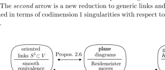
Thefirstdouble arrow in Figure 4 is a classical reduction of an equivalence of links to extended Reidemeister moves on plane diagrams in Figure 5.

Thesecondarrow is a new reduction to generic links and generic equivalence defined in terms of codimension 1 singularities with respect to the rotation of links inV.

The third arrow is a reformulation of the previous reduction in terms of canonical loops of links in the space of all links in the solid torusV.

The fourth arrow is a reduction of generic links to their 2-dimensional diagram surfaces considered up to 3-dimensional moves in Figure 10.

The fifth arrow is a final reduction of generic links to their trace graphs considered up to equivalence generated by the moves in Figure 11.

The key ingredient of the proofs is a description of versal deformations and bifurcation diagrams of codimension 2 multi local singularities of plane curves in Section 4.

ACKNOWLEDGEMENTS. The second author is especially grateful to Hugh Morton and Farid Tari for fruitful comments and suggestions. He also thanks Yu. Burman, M. Kazaryan, V. Vassiliev, V. Zakalyukin for useful discussions.

2. Singular subspaces in the space of all links. 2.1. Codimension 1 singularities of link diagrams. Let M; N be smooth finite dimensional manifolds. Denote by Jk

½l&ðM; NÞthe

space of alll-tuplek-jets of smooth maps #:M !N for all tuples ðu1;+ + +; ulÞ2 Ml_{, see [1, Sections I.2]. Letðx}

1;+ + +; xmÞandðy1;+ + +; ynÞbe local coordinates inM

and N, respectively. If the map # is defined locally by yj¼#jðx1;+ + +; xnÞ, j¼1;+ + +; m, then the l-tuple k-jet of the map # at a point ðu1;+ + +; ulÞ is

determined by

fx1;+ + +; xmg; fy1;+ + +; yng; @#j @xi

! "

; . . . @

k_# j @xi1+ + +@xis

! "

; i1þ + + + þis¼k:

The above quantities define local coordinates in Jk

½l&ðM; NÞ. The l-tuplek-jet jk

½l&# of a smooth map #:M !N can be considered as the map jk½l&#:Ml!

Jk

½l&ðM; NÞ, namelyðu1;+ + +; ulÞgoes to thel-tuplek-jet of the map#atðu1;+ + +; ulÞ.

Take an open set W 'Jk

½l&ðM; NÞfor some k; l. The set of smooth maps f :

M!N with l-tuple k-jets from W is calledopen. These sets for all openW ' Jk

½l&ðM; NÞ form a basis of theWhitneytopology in C1ðM; NÞ. So two maps are

close in the Whitney topology if they are close with all theirs derivatives. DEFINITION2.1. The space SL of all links K'V inherits the Whitney

topology from C1ðFmj¼1S1j; VÞ. A link K defined by a smooth embedding f:Fm_j¼1S1

j !V is called general if the diagram D¼prxzðKÞ 'Axz is general,

, the map prxz0f :

Fm

j¼1Sj1!Axz is a smooth embedding outside finitely

many doublecrossings, an overcrossing arc is specified at each crossing; , the extrema of prz:D!Sz1 are not crossings and have distinct z

-coor-dinates.

Denote by!ð0Þ'SLthe subspace of all general links.

We consider local singularities, so fix coordinates x; zaround each point in Axz. Thex-axis is said to behorizontal, i.e. it is perpendicular to the vertical core S1

z'Axz. Classical codimension 1 singularities of plane curves were described by

David [5, List I on p. 561], namely the ordinary cusp (the A2 singularity in Arnold’s notations), simple tangency (A3) and triple point (D4). The solid torus V has the distinguished vertical direction along S1

z, so we also consider

singularities with respect toprz:V !S1z, e.g. Reidemeister move IV is generated

by passing through a critical crossing , where one of the tangents is horizontal. DEFINITION2.2. AdiagramDis the image of a smooth mapg:Fm_j¼1S1

j!Axz.

A triple pointof the diagram Dis a transversal intersectionp of 3 arcs such that all the tangents atpare not horizontal.

Asimple tangency is an intersectionpof 2 arcs given locally by u¼ -v2_{. We} assume that the tangent atp is not horizontal.

Anordinary cuspis the singular pointpof an arc given locally byu2_¼v3_{. We} assume that the tangent atp is not horizontal.

Acritical crossingis a transversal intersectionpof 2 arcs such that one of the tangents atp is horizontal.

A cubical point is the singular point p of an arc given locally byz¼u3_{, the} tangent atp is horizontal.

A mixed pair is a pair of a local maximum and a local minimum of the projectionprz:D!Sz1, lying in the same horizontal line.

Anextreme pairis a pair of either 2 local maxima or 2 local minima of the projectionprz:D!S1z, lying in the same horizontal line.

Given a singularity $2 f ; ; ; ; ; ; g, denote by !$ 'SL the

singular subspace consisting of all links K'V such that prxzðKÞ is general

outside$.

2.2. Extended Reidemeister theorem.

DEFINITION2.3. Let M be a finite dimensional smooth manifold. A subspace"'M is calleda stratified space if " is the union of disjoint smooth submanifolds"i_{(strata) such that the boundary of each stratum is a finite union}

of strata of less dimensions. LetNbe a finite dimensional manifold. A smooth map #:M!N is transversal to a smooth submanifoldU'N if the spacesf*ðTxMÞ

and TfðxÞU generate TfðxÞN for each x2M. A smooth map is %:M!N transversal to a stratified space "'N if the the map % is transversal to each stratum of".

Briefly Theorem 2.4 says that any map can be approximated by ‘a nice map’. THEOREM2.4 (Multi-jet transversality theorem of Thom, see [1, Section I.2]). Let M; N be compact smooth manifolds, "'Jk

½l&ðM; NÞ be a stratified

space. Given a smooth map#:M!Nthere is a smooth map%:M !Nsuch that

, the map%is arbitrarily close to #with respect to the Whitney topology;

, thel-tuple k-jet jk

½l&%:Ml!J½kl&ðM; NÞis transversal to "'J½kl&ðM; NÞ.

LEMMA2.5.

(a)The subspace!ð1Þ _{has codimension 1 in the spaceSL.}

(b)The subspace!ð0Þ_{is open and dense in the spaceSL.}

Sketch:

(a) It is a standard computation in the spaceJ1

½3&ðR;R2Þof 3-tuple 1-jets of maps

ðxðrÞ; zðrÞÞ:R!R2_{. For instance, fixing 3 parameters r}

1; r2; r3, the subspace ! maps to the subspace of J1

½3&ðR;R

2_{Þ given by 4 equations xðr} 1Þ ¼

xðr2Þ ¼xðr3Þ, zðr1Þ ¼zðr2Þ ¼zðr3Þand 3 inequalities z_ðriÞ6¼0, i¼1;2;3,

mean-ing that the tangents are not horizontal, hence the codimension of the subspace ! 'SL is 1 after forgetting the 3 parameters. Analogously ! maps to the subspace given by 4 equations x_ðr1Þ ¼z_ðr1Þ ¼0, r1¼r2¼r3, hence the codi-mension of! 'SLis 1. A similar detailed argument will be given in the proof of Lemma 3.5.

(b) The conditions of Definition 2.1 define an open subset ofSLwhose complement is clearly the closure of the codimension 1 subspace!ð1Þ_{from Definition 2.2.}

PROPOSITION2.6. Any smooth link can be approximated by a general link. General links areisotopicif and only if their diagrams can be obtained from each other by a plane isotopy and finitely many Reidemeister moves in Figure 5.

In Figure 5, orientations of arcs and symmetric images of the moves are omitted.

2.3. The co-orientation of codimension 1 subspaces.

Using Gauss diagrams of link diagrams, we define the co-orientation of codimension 1 subspaces! ;! ;! ;! from Definition 2.2.

DEFINITION2.7. Let a general link K be defined by f :Fjm¼1Sj1!V. The Gaussdiagram GDðKÞis the union Fm_j¼1S1

j with chords connecting pointss1; s2 such that prxzðfðs1ÞÞ ¼prxzðfðs2ÞÞ. Gauss diagrams GD1;GD2 are equivalent if there is an orientation preserving diffeomorphism of Fm_j¼1S1

j such that the

endpoints of any chord ofGD1map onto the endpoints of a chord ofGD2and vice versa.

DEFINITION2.8. For each of 2 types of oriented triple points, the co-orientationof! is defined in terms of the Gauss diagrams of the corresponding linksK-in Figure 6. Assume that, whilet2St1increases, the pointrottðKÞ2SL

passes through! from the negative side to the positive one. Then associate to the corresponding triple vertex ofTGðKÞthepositivesign þ, otherwise take the

negative sign %. The co-orientations of ! , ! , ! are similarly defined in Figure 6.

Look at the trefoil K in Figure 2 and its trace graph TGðKÞ in Figure 3. Consider the first triple vertex of TGðKÞ at the critical moment t1 2ð"=4;"=2Þ. The knotrot"=4ðKÞis on the positive side of! (the 1st type in Figure 6), while rot"=2ðKÞis on the negative side of! , i.e. the first triple vertex has the positive sign. At the second triple vertex fort22ð"=2;3"=4Þ, the knotrottðKÞgoes from the

3. Generic links, equivalences, loops and homotopies. 3.1. The canonical loop of a link and generic links.

Generic links will be defined as the most generic points in the spaceSLof all linksK'V with respect to the rotationrottof the solid torus V.

DEFINITION3.1. ThecanonicalloopCLðKÞ 'SLof a smooth linkK'V is the union of the rotated linksrottðKÞ2SLover allt2St1.

A link K'V isgenericif there are finitely manyt1;+ + +; tk2St1 such that

, for allt =2 ft1;+ + +; tkg, the linksrottðKÞare general, i.e.rottðKÞ2!ð0Þ;

, CLðKÞ transversally intersects ! S! S! S! at each t2 ft1;+ + +; tkg.

Denote by#ð0Þ_{'SLthe subspace of all generic links inV.}

Morse modifications of index 1 would change the trace graph dramatically. Luckily following Lemma 3.2 shows that they can not occur under strong equivalence. More exactly Lemma 3.2 shows that the canonical loopCLðKÞnever touches the subspace! S! S! for any linkK. Therefore the transversality from the last condition of Definition 3.1 is relevant only for the subspace! .

LEMMA3.2 (Main topological lemma). For any linkK'V, the canonical loopCLðKÞdoes not touch the subspace ! S! S! . More formally, if K2

!$ for$¼ ; ; , the linksrot-"ðKÞare on different sides of!$ for small" >0.

PROOF. For the subspaces ! and ! , the projections of two small arcs with a tangent point (respectively, a cusp) are interchanged under the rotation. Figure 6 shows that the links rot_-"ðKÞare on different sides of! and! ,

respectively, since the tangent at p is not horizontal, i.e. not orthogonal to the vertical axis S1

z. The argument for ! is the same, since one tangent at the

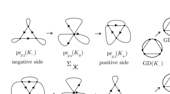
critical crossing is not horizontal, see the last picture of Figure 6. ! EXAMPLE3.3. The canonical loop CLðKÞ of a knot K'V can touch the subspace! . Consider the three arcsJ1; J2; J3'R3defined by (see Figure 7 below)

x1¼&u2;

y1¼0;

z1¼u; 8 > < > :

x2¼u;

y2¼ %1;

z2¼u; 8 < :

x3¼ %u;

y3¼1;

z3¼u; 8 <

: u2R; & >0:

Under the compositionprxz0rott, the arcsJ1; J2; J3map to the following ones:

where z1; z2; z3 are constants. For small t¼" >0, the double crossing p23¼ prxzðrot"ðJ2ÞÞTprxzðrot"ðJ3ÞÞhas the coordinates x¼0, z¼ %tan". Then p23 is at the left of the first rotated arcx1ðtÞ ¼&z21costwith respect toX.

Fort¼ %" <0, the crossing withx¼0,z¼tan"is also at the left of the first arc. Take a knot K2! containing small parts of the arcs described above. Thenrot-"ðKÞare on the same side of! . This means that, under the rotation of K, Reidemeister move III is not performed for the diagramprxzðrottðKÞÞ.

3.2. Codimension 2 singularities and generic equivalences.

Classical codimension 2 singularities of plane curves were described by David [5, List II on p. 561], namely the ramphoidal cusp (the A4 singularity in Arnold’s notations), intersected cusp (D5), tangent triple point (D4), cubic tangency (A5) and ordinary quadruple point (X9). We need to distinguish more refined singularities since the canonical loop of a link may not be transversal to some singular subspace, e.g. it is transversal to the codimension 2 subspace of horizontal cusps! , but not to the codimension 1 subspace of all cusps! S! . All tangents below are nothorizontalunless stated otherwise.

DEFINITION3.4 (codimension 2 singularitiesof link diagrams). LetDbe a diagram, i.e. the image of a smooth mapg:Fm_j¼1S1

j !Axz.

Aquadruple pointof Dis a transversal intersectionpof 4 arcs.

Atangent triple pointofDis an intersectionpof 3 arcs, the first two arcs have a simple tangency and do not touch the third arc.

Anintersected cuspofDis an intersection of 2 arcs, where the first arc has an ordinary cusp whose vectorð€x;€zÞdoes not touch the second arc.

Acubic tangency is an intersection of 2 arcs given locally byu¼0, u¼v3_. Aramphoidal cusp is the singular point of an arc, given locally byu2_¼v5_. A horizontal cuspis an ordinary cusp with horizontal tangent.

Amixed tangencyis a simple tangency with a horizontal tangent such that one of the extrema is a maximum, another one is a minimum.

Anextreme tangencyis a simple tangency with a horizontal tangent such that both extrema are either maxima or minima.

; Ahorizontal triple pointis a triple intersection, where the tangent line of the first arc is horizontal, the tangent lines of the other arcs are not horizontal.

Given a singularity '2 f ; ; ; ; ; ; ; ; ; g, denote by !' the

union of all linksK'V such that the diagram prxzðKÞis general outside'. Set

!ð2Þ¼! [! [! [! [! [! [! [! [! [! 'SL:

LEMMA3.5. The singular subspace!ð2Þ_{has codimension 2 in the spaceSL.}

PROOF. We use multi-jets of mapsðxðrÞ; zðrÞÞ:R!R2defining a diagram

D. Fixing 4 points r1; r2; r3; r4, each singularity ' from Definition 3.4 can be described in terms of 4-tuple 3-jets from the spaceJ3

½4&ðR;R

2

Þ, where each point has the 36 coordinates:

J_½3_4&ðR;R2Þ: ri;

xðriÞ; zðriÞ; x_ðriÞ; z_ðriÞ;

€

xðriÞ; z€ðriÞ; ...xðriÞ; ...zðriÞ;

i¼1;2;3;4:

(

The jets over all K2#' form the finite dimensional subspace !~'' J3

½4&ðR;R

2_{Þ. A simple tangency of 2 arcs at r}

i; rj is described by %ij¼

_

xðriÞ x_ðrjÞ

_

zðriÞ z_ðrjÞ

# # # # # # #

#¼0:The frequent inequalityz_ðriÞ6¼0below says that the tangent

ofDatriis not horizontal. The stringr16¼r26¼r36¼r4will mean thatr1; r2; r3; r4 are pairwise disjoint.

~

! xðr1Þ ¼xðr2Þ ¼xðr3Þ ¼xðr4Þ; zðr1Þ ¼zðr2Þ ¼zðr3Þ ¼zðr4Þ; (

r16¼r26¼r36¼r4; _

zðriÞ6¼0; %ij6¼0; i6¼j;

~

! xðr1Þ ¼xðr2Þ ¼xðr3Þ; zðr1Þ ¼zðr2Þ ¼zðr3Þ; (

r16¼r26¼r3¼r4; z_ðriÞ6¼0;

%12¼0; %236¼0; %136¼0;

~

! xðr1Þ ¼xðr2Þ; zðr1Þ ¼zðr2Þ; _

xðr1Þ ¼z_ðr1Þ ¼0; (

€

zðr1Þ6¼0; z_ðr2Þ6¼0;

r16¼r2¼r3¼r4; €

xðr1Þ x_ðr2Þ €

zðr1Þ z_ðr2Þ # # # # # # # #6¼0;

~ !

xðr1Þ ¼xðr2Þ; zðr1Þ ¼zðr2Þ;

r16¼r2¼r3¼r4; %12¼0; _

zðr1Þ6¼0; z_ðr2Þ6¼0; 8 > < > : €

xðr1Þ x_ðr2Þ €

zðr1Þ z_ðr2Þ # # # # # # # #¼0;

x ...

ðr1Þ x_ðr2Þ

z ...

~

! x_ðr1Þ ¼z_ðr1Þ ¼0; €zðr1Þ6¼0; r1¼r2¼r3¼r4; (

€

xðr1Þ ...xðr1Þ €

zðr1Þ ...zðr1Þ # # # # # # # # # #¼0;

~

! [!~ xðr1Þ ¼xðr2Þ ¼xðr3Þ;

zðr1Þ ¼zðr2Þ ¼zðr3Þ; (

_

zðr1Þ ¼0; z€ðr1Þ6¼0; _

zðr2Þ6¼0; z_ðr3Þ6¼0;

r16¼r26¼r3¼r4; %ij6¼0; i6¼j;

~

! fx_ðr1Þ ¼z_ðr1Þ ¼z€ðr1Þ ¼0; r1¼r2¼r3¼r4; ...zðr1Þ6¼0;

~

! [!~ zðr1Þ ¼zðr2Þ; z_ðr1Þ ¼z_ðr2Þ ¼0; xðr1Þ ¼xðr2Þ; r16¼r2 ¼r3¼r4; (

€

zðr1Þ6¼0; €

zðr2Þ6¼0;

The conditions above can be obtained using classical normal forms of the singularities, e.g. the ramphoidal cusp is a degeneration of the ordinary cusp clearly given by x_ðrÞ ¼z_ðrÞ ¼0. Locally one has ðx; zÞ ¼ ða2r2þa3r3þ + + +; b2r2þb3r3þ + + +Þ, b26¼0, which is (left) equivalent to ðx; zÞ ¼ ðða3%b3a2=b2Þr3þ + + +; b2r2þ + + +Þ, hence a2b3¼b2a3, i.e. the vectors ð€xðrÞ;€zðrÞÞ andð...xðrÞ; z...ðrÞÞare collinear.

Each subspace!~'is defined by 6 equations, hencecodim ~#'¼6inJ_½3_4&ðR;R3Þ.

The subspaces !' from Definition 3.4 map to the corresponding subspaces !~'' J3

½4&ðR;R

2_{Þ by adding 4 points r}

1; r2; r3; r4 on a diagram. When we forget these points, the codimension decreases by 4, i.e.codim!'¼2in the spaceSL. !

DEFINITION3.6. Let# be the set of all links failing to be generic due to exactly one tangency ofCLðKÞwith the codimension 1 subspace! .

Given '2 f ; ; ; ; ; ; ; ; ; g, let #' consist of all linksK

failing to be generic because of exactly one transversal intersection ofCLðKÞwith !'. Set

#ð1Þ¼# [# [# [# [# [# [# [# [# [# [# :

Ageneric equivalence is a smooth pathF :½0;1&!SLintersecting transversally the subspace#ð1Þ_{, i.e. there are finitely manyr}

1;+ + +; rk2½0;1&such that

, the linksFðrÞ2SLare generic for allr =2 fr1;+ + +; rkg;

, the canonical loopCLðFðrÞÞtransversally intersects#ð1Þ_{for r¼r1;+ + +; rk.}

LEMMA3.7.

(a)The subspace#ð1Þ _{has codimension 1 in the spaceSL.}

(b)The subspace#ð0Þ_{is open and dense in the spaceSL.}

PROOF.

(a) Choose a linkK'V given by an embeddingf :Fm_j¼1S1

j !V that fails to be

were introduced using the rotation of the solid torusV. So we describe them in terms of mapsR!R3, notR!R2 as in the proof of Lemma 3.5.

There is a 4-tupleðr1; r2; r3; r4Þ2ðFmj¼1S1jÞ

4

defining the chosen singularity of

K2#'. The 4-tuple 3-jetj3_½4&fðr1; r2; r3; r4Þis a point inJ_½3_4&ðR;R3Þ. These points over allK2#'form the finite dimensional subspace#~''J_½3_4&ðR;R3Þ.

We check that#~'has codimension 5 inJ_½3_4&ðR;R3Þ. Denote byxðrÞ; yðrÞ; zðrÞ

the compositions off:Fm_j¼1S1

j !V 'R3 and the projections to the coordinate

axes. Then the 4-tuple 3-jet ofKis determined by the following 52 quantities.

J3

½4&ðR;R3Þ: ri;

xðriÞ; yðriÞ; zðriÞ; x_ðriÞ; y_ðriÞ; z_ðriÞ;

€

xðriÞ; y€ðriÞ; €zðriÞ; ...xðriÞ; ...yðriÞ; ...zðriÞ;

i¼1;2;3;4:

(

Fori; j2 f1;2;3;4g,i6¼j, introduce the differences

&xij¼xðriÞ %xðrjÞ; &yij¼yðriÞ %yðrjÞ; &zij¼zðriÞ %zðrjÞ:

PointsfðriÞ; fðrjÞ; fðrkÞ2Kproject to the same point underprxz: rottðKÞ!

Axz#ftgfor sometif and only ifzðriÞ ¼zðrjÞ ¼zðrkÞ,

&xij &xjk

&yij &yjk

# # # # # # #

#¼0:The last determinant is (up to the sign) the area of the triangle with the vertices ðxðriÞ; yðriÞÞ, ðxðrjÞ; yðrjÞÞ, ðxðrkÞ; yðrkÞÞ in the horizontal plane

fzðriÞ ¼zðrjÞ ¼zðrkÞg.

Set &ij¼

_

xðriÞ x_ðrjÞ &xij

_

yðriÞ y_ðrjÞ &yij

_

zðriÞ z_ðrjÞ &zij

# # # # # # # # # # #

#: The diagram prxzðrottðKÞÞ contains two arcs having a simple tangency atr¼ri, r¼rj and some t if and only ifzðriÞ ¼ zðrjÞand &ij¼0, i.e. the straight line throughfðriÞ; fðrjÞ2K lies in the plane

spanned by the tangent vectors ofKat r¼ri andr¼rj.

We describe analytically the subspaces #~' associated to the singularities

; ; ; ; ; ; ; ; ; ; :

~ #

zðr1Þ ¼zðr2Þ ¼zðr3Þ ¼zðr4Þ;

r16¼r26¼r36¼r4; _

zðriÞ6¼0; i¼1;2;3;4;

8 > < > :

&x12 &x23 &y12 &y23 # # # # # # # # # #¼

&x12 &x24 &y12 &y24 # # # # # # # # # #¼0; &ij6¼0; i; j2 f1;2;3;4g; i6¼j;

~ #

zðr1Þ ¼zðr2Þ ¼zðr3Þ;

r16¼r26¼r3¼r4; _

zðriÞ6¼0; i¼1;2;3;

8 > < > :

&x12 &x23 &y12 &y23 # # # # # # # # # #¼0;

~ #

zðr1Þ ¼zðr2Þ; _

zðr1Þ ¼0; z€ðr1Þ6¼0; _

zðr2Þ6¼0; 8 > < > : _

xðr1Þ x_ðr2Þ _

yðr1Þ y_ðr2Þ # # # # # # # # # #¼0; r16¼r2¼r3¼r4;

€

xðr1Þ x_ðr2Þ &x12 €

yðr1Þ y_ðr2Þ &y12 €

zðr1Þ z_ðr2Þ &z12 # # # # # # # # # # # # # # 6 ¼0; ~ #

zðr1Þ ¼zðr2Þ; &12¼0;

r16¼r2¼r3 ¼r4; _

zðr1Þ6¼0; z_ðr2Þ6¼0; 8 > < > : €

xðr1Þ x€ðr2Þ &x12 €

yðr1Þ y€ðr2Þ &y12 €

zðr1Þ z€ðr2Þ &z12 # # # # # # # # # # # # # # ¼0; ~

# z_ðr1Þ ¼0; z€ðr1Þ6¼0; r1¼r2¼r3¼r4; (

x ...

ðr1Þ € xðr1Þ ¼

y ...

ðr1Þ € yðr1Þ ¼

z ...

ðr1Þ € zðr1Þ

:

The last equations with 3 fractions mean that the vectors of the 2nd and 3rd derivatives are collinear, which corresponds to the similar condition for!~ in the proof of Lemma 3.5. If a denominator is zero, the numerator must be also zero.

~

# [#~ zðr1Þ ¼zðr2Þ ¼zðr3Þ; r16¼r26¼r3¼r4; _

zðr1Þ ¼0; z€ðr1Þ6¼0; z_ðr2Þ6¼0; z_ðr3Þ6¼0; (

&x12 &x23 &y12 &y23 # # # # # # # # # #¼0; ~

# fz_ðr1Þ ¼z€ðr1Þ ¼0; r1 ¼r2¼r3 ¼r4; ...zðr1Þ6¼0;

~

# [#~ zðr1Þ ¼zðr2Þ;

_

zðr1Þ ¼z_ðr2Þ ¼0; (

r16¼r2¼r3¼r4; €

zðr1Þ6¼0; z€ðr2Þ6¼0:

If z_ðriÞ6¼0, then locally ri can be considered as a function of z, hence any

function of (several)rican be differentiated with respect toz. Below the tangency

with ! means that the derivative of the vanishing determinant &¼ &_&x_y12 &x23

12 &y23 # # # # # # #

#defining a triple point under the projection prxz: rottðKÞ!

Axz#ftg also vanishes.

~ #

zðr1Þ ¼zðr2Þ ¼zðr3Þ; r1 6¼r26¼r3¼r4

&¼ d dz&¼0;

d2

dz2&6¼0; &¼

&x12 &x23 &y12 &y23 # # # # # # # # # #;

&ij6¼0; i6¼j;

_

zðriÞ6¼0:

8 > < > :

Generic inequalitiesdg=dz6¼0should be added to the descriptions above for each condition g¼0, which guarantees no tangency of the canonical loop with the corresponding subspace!'. In important cases like#~ we explicitly accompanied

_

zðr1Þ ¼0withz€ðr2Þ¼6 0equivalent toz_ðr1ðzÞÞ=dz6¼0, but also every equation like

Each subspace#~'is defined by 5 equations, hencecodim ~#'¼5inJ_½3_4&ðR;R3Þ.

The subspaces#'introduced geometrically in Definition 3.6 correspond to#~'by

adding 4 points r1; r2; r3; r4 on a link. When we forget about these points the codimension decreases by 4, i.e.codim#'¼1 in the spaceSLof all links K'V.

(b) The conditions of Definition 3.6 define an open subset ofSLwhose complement is clearly the closure of the codimension 1 subspace#ð1Þ. ! The following result similar to Proposition 2.6 follows from Lemma 3.7 since by Theorem 2.4 any isotopy in the space SLof links can be approximated by a path transversally intersecting the singular subspace#ð1Þ_'SL.

PROPOSITION3.8.

(a)Any smooth link can be approximated by a generic link.

(b)Any smooth equivalence of links can be approximated by a generic one.

3.3. Generic loops and generic homotopies in the space of links. A loopof linksfKtg'SLmeans asmoothloop, i.e. a smooth mapS1t !SL.

Generic loops provide a suitable generalization of the canonical loop.

DEFINITION3.9. A smooth loop of linksfKtg'SL,t2St1, is calledgeneric

if there are finitely many critical momentst1;+ + +; tk 2S1t such that

, the linkKtmaps to Ktþ" under the rotation through"for every t2St1;

, for allt =2 ft1;+ + +; tkg, the linksKtare general, i.e.Kt2!ð0Þ;

, fKtgtransversally intersects! S! S! S! at eacht¼t1;+ + +; tk.

Due to Lemmas 2.5, 3.7 any loop can be approximated by a generic loop. But a generic loop may be too trivial. For instance, a loopS1

t !SLcontractible to a

generic link through generic links carries information about only one diagram. More interesting objects are generic loops homotopic to canonical loops.

DEFINITION3.10. A smooth family fLsg of loops, s2½0;1&, is called a generic homotopy if there are finitely many critical moments s1;+ + +; sk2½0;1&

such that

, fors =2 fs1;+ + +; skg, the loopLs is generic in the sense of Definition 3.9;

, for each s2 fs1;+ + +; skg, the loop Ls fails to be generic since either Ls

transversally intersects!ð2Þ _orL

stouches! at exactly one point.

LEMMA3.11.

(a)The canonical loop of any generic link is a generic loop.

(c)If canonical loops CLðK0Þ and CLðK1Þ of generic links K0 and K1 are

generically homotopic thenK0 and K1 are generically equivalent.

PROOF.

(a) The canonical loop of any link is symmetric in the sense thatrottðKÞmaps to

rottþ"ðKÞunder the rotation through "for every t2St1. The other conditions of

Definition 3.9 correspond to the conditions of Definition 3.1. (b) Compare Definition 3.6 with Definitions 3.9 and 3.10.

(c) LetfLsg,s2½0;1&, be a generic homotopy betweenCLðK0ÞandCLðK1Þ. The loopsLscan be represented by a cylinderS1t # ½0;1&mapped to the spaceSL. Take

a smooth path connectingK0andK1inside the cylinder. This smooth equivalence can be approximated by a generic one due to Proposition 3.8b. !

By Lemma 3.11 the classification of links reduces to their canonical loops. PROPOSITION3.12. Generic links are generically equivalent inV if and only if their canonical loops are generically homotopic in the spaceSLof all linksK'V.

4. Through codimension 2 singularities.

4.1. Versal deformations of codimension 2 singularities.

To understand what happens when the canonical loop of a link passes through the singular subspace!ð2Þ_{, we study bifurcation diagrams of}

codimen-sion 2 singularities.

LEMMA4.1. The codimension 2 singularities from Definition 3.4 have the normal forms in the table below, whereris the parameter on the curve and

, Ae is the extended right-left equivalence, i.e. diffeomorphisms of R2 don’t fix 0;

, Az is the restricted right-left equivalence such that left diffeomorphisms of

R2 have the formðgðx; zÞ; hðzÞÞ, where gðx; zÞ:R2 !R, hðzÞ:R!Rare diffeomorphisms.

Sketch: The normal forms up toAe-equivalence are classical, e.g. the parameter e6¼0 in the normal form of (X9) can not be skipped as the cross-ratio of 4 slopes is invariant under diffeomorphisms, see [14, Lemma 6.5]. The singularities , , , , should be considered up to Az-equivalence respecting

fz¼constg, otherwise they don’t have codimension 2, e.g. the normal form ðr2_{; r}3_{Þof is notA}

z-equivalent to the normal formðr3; r2Þof . Deducing new

normal forms is similar, e.g. the horizontal cusp is defined by the conditions _

,Ae fx¼0; z¼rg; fx¼r; z¼rg; fx¼ %r; z¼rg; fx¼er; z¼rg

,Ae fx¼r2; z¼rg; fx¼0; z¼rg; fx¼r; z¼rg

,Ae fx¼r3; z¼r2g; fx¼r; z¼rg

,Ae fx¼r3; z¼rg; fx¼0; z¼rg

,Ae fx¼r5; z¼r2g

,Az fx¼r2; z¼r3g

,Az fx¼r; z¼r2g; fx¼r; z¼ %r2g

,Az fx¼r; z¼ %2r2g; fx¼r; z¼ %r2g

,Az fx¼r; z¼ %r2g; fx¼r; z¼rg; fx¼ %r; z¼rg

,Az fx¼r; z¼ %r2g; fx¼r; z¼rg; fx¼2r; z¼rg

Mancini and Ruas [12] have shown that the group Az from Lemma 4.1 is

geometric in the sense of Damon [4]. So the standard technique of singularity theory can be applied to find versal deformations of corresponding codimension 2 singularities.

We consider horizontal triple points and separately, because the associated moves on trace graphs look slightly different in Figure 11ix, 11x. A deformation of a germ ðxðrÞ; zðrÞÞ:R!R2 with parameters a; b is a germ F :

R#R2_!R2 _{such that Fðr; 0;0Þ 1 ðxðrÞ; zðrÞÞ. A deformationF isversal if any} other deformation can be obtained fromF by actions of the corresponding group

AeorAz.

The versality can be checked using the following tangent spaces at germs in the space of deformations. LetTr_{be therighttangent space at a germðxðrÞ; zðrÞÞ}

generated by the right diffeomorphismsR!R, e.g. the right spaceTr_atðr5_{; r}2_Þ of consists ofð5r4_{fðrÞ;2rfðrÞÞ, wheref :R!R. Denote byT}l_{thelefttangent}

space at a germ ðxðrÞ; zðrÞÞ generated by the restricted left diffeomorphisms ðgðx; zÞ; hðzÞÞ:R2!R2, where g:R2!R, h:R!R are any germs. For instance, the left space Tl _{at ðr}2_{; r}3_{Þ of is formed by ðgðr}2_{; r}3_{Þ; hðr}3_{ÞÞ ¼} ða1þa2r2þa3r3þ + + +; b1þb2r3þ + + +Þ. The parameter normal space Np of a deformation Fðr;a; bÞ consists of linear combinations cð@F =@aÞ þdð@F =@bÞ at

a¼b¼0, wherec; dare constants, e.g. the spaceNp_ofðr5_þar3_{þbr; r}2_Þconsists of vectorsðcr3_þdr;0Þ.

In the case of a multi-germ the right spaceTr

i is associated to the independent

right diffeomorphismsfiðrÞaround each pointri. The left spaceTilis generated by

the same left diffeomorphisms at everyri. The parameter spaceNipis spanned by

the derivatives along the parameters of the deformation at eachri.

PROPOSITION4.2. A deformation Fðr;a; bÞ of a multi-germ ðxðrÞ; zðrÞÞ:

R!R2is versal if at every pointriany germR!R2can be represented as a sum of vectors from the spacesTr

i,Til andN p i.

LEMMA4.3. The codimension 2 singularities from Definition 3.4 have the versal deformations with parametersa; bin the table below.

,Ae fx¼0; z¼rg;fx¼rþa; z¼rg;fx¼ %r%b; z¼rg;fx¼er; z¼rg

,Ae fx¼r2%2a; z¼rg; fx¼0; z¼rg; fx¼r%b; z¼rg

,Ae fx¼r3%br; z¼r2g; fx¼r%a; z¼rg

,Ae fx¼r3%3brþa; z¼rg; fx¼0; z¼rg

,Ae fx¼r5þar3þbr; z¼r2g

,Az fx¼r2; z¼r3þar2%brg

,Az fx¼r; z¼r2%bg; fx¼rþa; z¼ %r2g

,Az fx¼r; z¼ %2r2%bg; fx¼rþa; z¼ %r2g

,Az fx¼r; z¼ %r2g; fx¼rþa; z¼rg; fx¼ %r%b; z¼rg

,Az fx¼r; z¼ %r2g; fx¼rþa; z¼rg; fx¼r=2%b; z¼rg

Sketch: Versal deformations of classical codimension 2 singularities (A4), (D5), (D4), (A5) and (X9) up to Ae-equivalence were recently described

by Wall [14, Subsection 6.1]. The remaining cases follow from the table below.

singularity Tir Til N

p i

ð2rfðrÞ;3r2_{fðrÞÞ ðgðr}2_{; r}3_{Þ; hðr}3_{ÞÞ ð0; cr}2_%drÞ ðf1ðrÞ;2rf1ðrÞÞ ðgðr; r2Þ; hðr2ÞÞ ð0;%dÞ ðf2ðrÞ;%2rf2ðrÞÞ ðgðr;%r2Þ; hð%r2ÞÞ ðc;0Þ ðf1ðrÞ;%4rf1ðrÞÞ ðgðr;%2r2Þ; hð%2r2ÞÞ ð0;%dÞ ðf2ðrÞ;%2rf2ðrÞÞ ðgðr;%r2Þ; hð%r2ÞÞ ðc;0Þ ðf1ðrÞ;%2rf1ðrÞÞ ðgðr;%r2Þ; hð%r2ÞÞ ð0;0Þ ðf2ðrÞ; f2ðrÞÞ ðgðr; rÞ; hðrÞÞ ðc;0Þ ð%f3ðrÞ; f3ðrÞÞ ðgð%r; rÞ; hðrÞÞ ð%d;0Þ ðf1ðrÞ;%2rf1ðrÞÞ ðgðr;%r2Þ; hð%r2ÞÞ ð0;0Þ ðf2ðrÞ; f2ðrÞÞ ðgðr; rÞ; hðrÞÞ ðc;0Þ ð%f3ðrÞ=2; f3ðrÞÞ ðgð%r=2; rÞ; hðrÞÞ ð%d;0Þ

Case vi of a horizontal cusp . By Proposition 4.2 we should prove that any germ ðxðrÞ; zðrÞÞ:R!R2_{can be represented as a sum of vectors from the spacesT}r

and N₁p, i.e. we solve the functional equations from the table xðrÞ ¼2rfðrÞ þ gðr2_{; r}3_{ÞandzðrÞ ¼ %drþcr}2_þ3r2_{fðrÞ þhðr}3_{Þ, which have one the of the possible} solutions

d¼ %z_ð0Þ; hðr3Þ ¼zð0Þ; fðrÞ ¼ zðrÞ %z_ð0Þr%zð0Þ

3r2 þ

_

xð0Þ 2 %

€ zð0Þ

6 ;

c¼z€ð0Þ %3 _xð0Þ 2 ; gðr

2_{; r}3

Þ ¼xðrÞ %x_ð0Þr%2zðrÞ %€zð0Þr

2_{=2%z_ð0Þr%zð0Þ}

3r :

8 > > < > > :

Herehhas only the constant term andgðr2_{; r}3_{Þhas no linear term inr, all other} powers have the form2jþ3kfor some integersj; k!0, e.g.

for a germða0þa1rþa2r2þ + + +; b0þb1rþb2r2þ + + +Þone has

f ¼a1=2þ + + +; gðx; zÞ ¼a0þa2xþ + + +; h¼b0; d¼ %b1; c¼ ð2b2%3a1Þ=2:

Case vii of a mixed tangency . We prove that at each pointri,i¼1;2, any germ

ðxi; ziÞ:R!R2 can be represented as a sum of vectors from Tir, Til,N p i, i.e. in

terms of suitablec; dandf,g,h. Write down the equations from the table above.

x1ðrÞ ¼f1ðrÞ þgðr; r2Þ; z1ðrÞ ¼2rf1ðrÞ þhðr2Þ %d;

x2ðrÞ ¼cþf2ðrÞ þgðr;%r2Þ; z2ðrÞ ¼ %2rf2ðrÞ þhð%r2Þ: (

ð Þ

For a function fðrÞ denote its constant term simply by f. The equations

z1ðrÞ ¼2rf1ðrÞ þhðr2Þ %dandz2ðrÞ ¼2rf2ðrÞ þhð%r2Þin degree 1 determine the constant terms f1; f2 of f1ðrÞ; f2ðrÞ. Then system ð Þ in degree 0 has a unique solution:

x1¼f1þg; z1¼h%d;

x2¼cþf2þg; z2¼h: (

g¼x1%f1; h¼z2;

c¼x2%x1þf1%f2; d¼z2%z1: (

ð 0Þ

For a functionfðrÞdefine its odd and even part asOddfðrÞ ¼ ðfðrÞ %fð%rÞÞ=2, EvenfðrÞ ¼ ðfðrÞ þfð%rÞÞ=2. We look for solutions gðx; zÞ ¼g1ðxÞ þg2ðzÞ and

The resulting system has a solution below, where Evenz1ðrÞ %Evenz2ðrÞ þdis divisible byrdue to ( 0). So the deformation is versal by Proposition 4.2.

Evenf1ðrÞ ¼Oddz1ðrÞ=2r; Evenf2ðrÞ ¼ %Oddz2ðrÞ=2r;

Oddf1ðrÞ ¼ ðEvenz1ðrÞ %Evenz2ðrÞ þdÞ=4rþ ðOddx1ðrÞ %Oddx2ðrÞÞ=2; Oddf2ðrÞ ¼ ðEvenz1ðrÞ %Evenz2ðrÞ þdÞ=4rþ ðOddx2ðrÞ %Oddx1ðrÞÞ=2; Eveng1ðrÞ ¼ ðEvenx1ðrÞ þEvenx2ðrÞ %Oddz1ðrÞ=2rþOddz2ðrÞ=2r%cÞ=2; Oddg1ðrÞ ¼ ðEvenz2ðrÞ %Evenz1ðrÞ %dÞ=4rþ ðOddx1ðrÞ þOddx2ðrÞÞ=2;

g2ðr2Þ ¼ ðEvenx1ðrÞ %Evenx2ðrÞ %Oddz1ðrÞ=2r%Oddz2ðrÞ=2rþcÞ=2;

hðr2Þ ¼ ðEvenz1ðrÞ þEvenz2ðrÞ þdÞ=2þrðOddx2ðrÞ %Oddx1ðrÞÞ: 8 > > > > > > > > > > > > < > > > > > > > > > > > > :

Case viii of an extreme tangency is similar to Case vii. Case ix of a horizontal triple point . The table above gives

x1ðrÞ ¼f1ðrÞ þgðr;%r2Þ; z1ðrÞ ¼ %2rf1ðrÞ þhð%r2Þ;

x2ðrÞ ¼cþf2ðrÞ þgðr; rÞ; z2ðrÞ ¼f2ðrÞ þhðrÞ;

x3ðrÞ ¼ %d%f3ðrÞ þgð%r; rÞ; z3ðrÞ ¼f3ðrÞ þhðrÞ: 8 > < > : ð Þ

The equationz1ðrÞ ¼ %2rf1ðrÞ þhð%r2Þin degree 1 determines the constant term

f1 of the functionf1ðrÞ. Then system ð Þin degree 0 has a unique solution.

x1¼f1þg; z1¼h;

x2¼cþf2þg; z2¼f2þh;

x3¼ %d%f3þg; z3¼f3þh: 8

> < > :

g¼x1%f1; h¼z1;

f2¼z2%z1; c¼x2%x1þf1þz1%z2;

f3¼z3%z1; d¼x1%f1%x3þz1%z3: 8

> < > :

We look for gðx; zÞ ¼g1ðxÞ þg2ðzÞ. Apply elementary operations toð Þ 2rx1ðrÞ þz1ðrÞ ¼2rg1ðrÞ þ2rg2ð%r2Þ þhð%r2Þ;

x2ðrÞ %z2ðrÞ ¼cþg1ðrÞ þg2ðrÞ %hðrÞ;

x3ðrÞ þz3ðrÞ ¼ %dþg1ð%rÞ þg2ðrÞ þhðrÞ: 8

> < > : ð 1Þ

The functionsf1; f2; f3can be expressed in terms of the solutions ofð 1Þ. Split the 1st equation ofð 1Þinto the odd and even parts, then apply operations toð 1Þ:

2rOddx1ðrÞ þEvenz1ðrÞ ¼2rOddg1ðrÞ þhð%r2Þ;

2rEvenx1ðrÞ þOddz1ðrÞ ¼2rEveng1ðrÞ þ2rg2ð%r2Þ; ð 2Þ

x3ðrÞ þz3ðrÞ þx2ðrÞ %z2ðrÞ %2Evenx1ðrÞ %

Oddz1ðrÞ

r ¼c%dþ2g2ðrÞ %2g2ð%r

which determines the coefficients of g2ðrÞ ¼P1i¼0eiri splitting into parts as

follows. Taking the odd part, we computeeiwith all oddi, the consider terms with

powers4i and 4iþ2 separately, find all e4iþ2 and continue splitting into parts. Having foundg2ðrÞ, compute Eveng1ðrÞfrom ð 2Þand work outhðrÞ,Oddg1ðrÞ from

x2ðrÞ %z2ðrÞ %x3ðrÞ %z3ðrÞ ¼cþdþ2Oddg1ðrÞ %2hðrÞ; 2rOddx1ðrÞ þEvenz1ðrÞ ¼2rOddg1ðrÞ þhð%r2Þ;

(

excludingOddg1ðrÞand then splitting the result into parts as above. Case x of another horizontal triple point is similar to Case ix.

4.2. Bifurcation diagrams of codimension 2 singularities.

The bifurcationdiagram of a codimension 2 singularity 'from Definition 3.4 is formed by the pairs ða; bÞ2R2 from the versal deformation of ' from Lemma 4.3. We will describe curves representing codimension 1 subspaces !$

adjoined to!' in the spaceSLof all linksK'V.

Oriented arcs in bifurcation diagrams of Figure 8 are associated to canonical loops CLðK_-"Þ 'SL, where links K-" are close to a given link K0. At the zero

critical moment, the loopCLðK0Þdefines an arc through the originfa¼b¼0g. These arcs are transversal to the codimension 1 subspace!ð1Þ_{apart from the cases}

below. In Figure 8ix and 8x the canonical loopCLðKsÞis parallel to! ,! ,

! in the following sense: ifK2! , thenCLðKÞ '! S! . IfK2! _{, then} CLðKÞ '! S! . Similarly,K2! implies thatCLðKÞ '! S! .

LEMMA4.4. Figure 8 contains the bifurcation diagrams of the

codimen-sion 2 singularities ' : ; ; ; ; ; ; ; ; ; and shows how the

canonical loopsCLðK-"Þintersect the adjoined codimension 1 subspaces!$.

PROOF. In Cases i–v below the canonical loops transversally intersects all the singular subspaces since the tangents of intersecting arcs are not horizontal. Case i of a quadruple point . There are 4 singular subspaces ! intersecting each other transversally at the singular subspace! . Using the normal form of from Lemma 4.1, we show 4 subspaces in the bifurcation diagram of Figure 8i, namelyfa¼0g (branches 1, 2, 4 intersect),fb¼0g(branches 1, 3, 4 intersect),

Case iii of an intersected cusp . The branchðr3_{%br; r}2_{Þhas a self-intersection at}

r¼ -pffiffiffib,b!0, which becomes an ordinary cusp ifb¼0. The self-intersection is a triple point when it is on the branchðr%a; rÞ, i.e.a¼b. Finally, we get a simple tangency ofðr3_{%br; r}2_{Þandðr%a; rÞifa¼2r}3_%r2_{; b¼3r}2_{%2ror3a%2br¼r}2 has a double root, i.e.b2_{þ3a¼0. The bifurcation diagram of Figure 8iii contains} 1 parabola, 1 line and 1 ray meeting at 0.

Case iv of a cubic tangency . The branch ðr3_{%3brþa; rÞhas extrema of the}

x-coordinate atr¼ -pffiffiffib, which lie onð0; rÞifr3_{%3brþa¼0, i.e.a}2_¼4b3_{. The} only subspace! is adjoined to! in the bifurcation diagram of Figure 8iv. Case v of a ramphoidal cusp . The curveðr5_þar3_{þbr; r}2_{Þhas an ordinary cusp} whenx_¼z_¼0, i.e.r¼0andb¼0, and a self-tangency when5r4_þ3ar2_þb¼0 has two double roots, i.e. 9a2_{¼20b. The bifurcation diagram of Figure 8v} contains 1 parabola and 1 line touching each other at 0.

Case vi of a horizontal cusp . The curveðr2_{; r}3_þar2_{%brÞhas a crossing at-r,} hence r3_{¼br and r¼ -}p_bffiffiffi_{, b >0. This crossing is critical, i.e.}

_

z¼3r2_{þ2ar%b¼0, if b¼a}2_{. The critical point becomes degenerate, i.e.} €

z¼6rþ2a¼0, if b¼ %a2_{=3. The subspace ! of ordinary cusps, where} _

x¼z_¼0, is represented by fb¼0g. The bifurcation diagram of Figure 8vi shows 2 parabolas, 1 line and 1 ray meeting at 0. The arc associated to a canonical loop moves in the vertical direction and remains parallel to the parabola

fb¼ %a2_{=3grepresenting the subspace! .}

Case vii of a mixed tangency . The branch ðr; r2_{%bÞ touches ðrþa;%r}2_{Þ if}

r2_{%b¼ %ðr%aÞ}2

has a double root, i.e.a2_{¼2b. Both curves have extrema in the} same horizontal line when b¼0. The bifurcation diagram of Figure 8vii has 1 parabola and 1 line touching each other at 0.

Case viii of an extreme tangency . The branchðr;%2r2_{þbÞtouchesðrþa;%r}2_Þ if b%2r2_{þb¼ %ðr%aÞ}2 _{has a double root, i.e. 2a}2_{þb¼0. Both branches have} extrema in the same horizontal line whenb¼0. The branchðr;%2r2_þbÞpasses through an extremum ofðrþa;%r2_{Þat r¼0 ifb¼2a}2_{. The branchðrþa;%r}2_Þ passes through an extremum ofðr;%2r2_{þbÞatr¼0ifb¼ %a}2_{. The bifurcation} diagram of Figure 8vii has 3 parabolas and 1 line touching each other at 0. Case ix of a horizontal triple point . The branchesðrþa; rÞandð%r%b; rÞpass through the extremum ofðr;%r2_{Þatr¼0whena¼0andb¼0, respectively. The} crossing ofðrþa; rÞand ð%r%b; rÞat r¼ %ðaþbÞ=2 lies in the same horizontal line with the extremum of ðr;%r2_{Þ at r¼0 if aþb¼0. The branches ðr;%r}2_Þ, ðrþa; rÞ and ð%r%b; rÞ have a triple point if r¼ %r2_þa¼r2_{%b or} ða%bÞ2 ¼2ðaþbÞ, which is a parabola in the bifurcation diagram of Figure 8ix. The arc associated to a canonical loop is transversal to the subspaces, because only one tangent remains horizontal under the rotation.

5. The diagram surface of a link.

In this section the classification problem of generic links K'V reduces to their diagram surfaces DSðKÞ in the thickened torus T¼Axz#St1, Axz¼

½%1;1&x#S1z.

5.1. The diagram surface of a link and generic surfaces.

Briefly the diagram surface of a loopfKtgof links is the 1-parameter family of

the diagramsprxzðKtÞ 'Axz#ftg. This family can be considered as the union of

link diagrams, i.e. as a 2-dimensional surface in the thickened torusT¼Axz#S1t.

DEFINITION5.1. Let fKtg'SL be a loop of links. The diagram surface

DSðfKtgÞ 'Axz#S1t is formed by the diagrams prxzðKtÞ 'Axz#ftg, t2St1. If Kt are knots, DSðfKtgÞ is the torus S1#S1t mapped to the thickened torus

T¼Axz#St1. Thediagram surfaceDSðKÞof an oriented linkK'V consists of

the diagramsprxzðrottðKÞÞ 'Axz#ftg and is oriented by the orientations ofK

andS1

t.

Figure 9 shows vertical sections of DSðKÞ for a smoothed trefoil K from Figure 2, t2½0;"&. Each section is the diagram of a rotated trefoil rottðKÞ for

some t2S1

t. Local extrema of rottðKÞ form horizontal circles parallel to S1t.

Several arcs in Figure 9 are dashed or dotted, because they are invisible in the

x-direction.

By Definition 3.9 the shiftt7!tþ"maps the surfaceDSðfKtgÞto its image

under the symmetry in S1

z. Actually the link Ktþ" is obtained from Kt by the

symmetry rot", i.e. the diagrams prxzðKtþ"Þ and prxzðKtÞ are symmetric for all t2S1

t. For a generic loopfKtg, the vertical sections ofDSðKÞare the diagrams

prxzðKtÞ and allow the codimension 1 singularities ; ; ; only. It follows

from the fact that any critical point ofprz:Kt!S1z remains critical under rott.

For anyt2S1

t, the points fromKt

T

ðDxy#fz¼ -1gÞand the critical points

ofprz:Kt!S1zdivide thei-th component ofKtinto arcsAt;i;q,q¼1;+ + +; ni. The

total number of these arcs does not depend ontsince any critical pointat2Ktof

przremains critical whiletvaries. The union

S

atof the extrema ofprz:Kt!Sz1

for allt2S1

t splits intocritical circles Ci ofDSðfKtgÞ. The unionBi;q¼SAt;i;q

over allt2S1

t is called atrace bandofDSðfKtgÞ. The 3 trace bands in the bottom

picture of Figure 9 have different colours. The arcs At;i;q are monotonic with

respect to przt:Kt!Sz1#ftg. Then the trace bands project 1-1 under przt :

DSðfKtgÞ!Sz1#St1. Successive bandsBi;q,Biþ1;q meet at a critical circle.

Thesingularpoints ofDSðfKtgÞare crossings and codimension 1 singularities

of the diagrams prxzðKtÞ over all t2St1. A trace arc is an intersection of the

and critical crossings of link diagramsprxzðKtÞare calledtriplevertices, tangent

vertices, hanging vertices and critical vertices of DSðfKtgÞ, respectively. So a

trace arc may contain several vertices ofDSðfKtgÞin the usual sense.

Take a singular pointp2DSðKÞthat is not a vertex and does not belong to a critical circle ofDSðKÞ. Thenpis a double crossing of two arcsAt;i;qandAt;j;sin a

diagram prxzðKtÞ. If the arc At;i;q passes over (respectively, under) At;j;s then

associate topthelabelðqisjÞ(respectively, thereversedlabelðsjqiÞ). IfKtis a knot

then we miss the indicesi; j¼1 as in Figure 3.

Trace arcs of DSðfKtgÞend at hanging vertices, meet each other at critical

vertices and intersect at triple vertices. Each trace arc ofDSðKÞis the evolution trace of a double crossing inAxz#S1t whiletvaries. The label of a pointpdoes not

change whenppasses through tangent vertices and triple vertices.

The diagram surface can be defined for any loop of links and can be extremely complicated. The surfaces corresponding to generic loops are simple and play the role of general link diagrams in dimension 3. As in the case of links, we define a generic surface associated to a generic loop. A generic surface will be an immersed surface with all combinatorial features of diagram surfaces of generic loops. For any generic surface, a corresponding generic loop is constructed in Lemma 5.6.

DEFINITION5.2. DecomposeS1

i into arcsAi;1;+ + +; Ai;ni. Introduce thetrace

bandsBi;q¼Ai;q#St1,q¼1;+ + +; ni. AgenericsurfaceS is the image of a smooth

maph:ðFmi¼1Si1Þ #St1¼

Sm i¼1ð

Sni

q¼1BiqÞ!Axz#St1 such that Conditions (i)–(v)

hold

(i) Conditions onsymmetryand trace bands.

, undert7!tþ"the surfaceSmaps to its image under the symmetry inS1

z;

, each trace bandBi;q'S projects one-to-one underprzt:S!S1z#St1.

The surfaceS should be simple enough. More formally we require the following. (ii) Conditions onsectionsDt¼STðAxz#ftgÞ,t2St1.

There are finitely many critical momentst1;+ + +; tl2St1 such that

, for allt =2 ft1;+ + +; tlg, the sectionsfDtgare general diagrams;

, for eacht¼t1;+ + +; tl, the sectionDthas one of the singularities ; ; ; ;

, whiletpasses a critical moment, Dtchanges by a move I–IV in Figure 5.

Conditions (ii) on sections imply some restrictions on trace bands. These requirements can be stated independently to define trace arcs and critical circles. (iii) Conditions ontrace arcsand criticalcircles.

, atrace arcis an intersection of the interiors of 2 trace bandsBi;qand Bj;s;

, acriticalcircleCi;qis the common boundary of successive bandsBi;q,Bi;qþ1.

The arcs defined above allow us to introduce vertices of a generic surfaceS. (iv) Conditions onvertices.

, a triplevertex is a transversal intersection of 3 trace bandsBi;q; Bj;s; Bk;r;

, a hangingvertex ofS is the endpoint of a trace arc inBi;qTBi;qþ1;

, a criticalvertex is the intersection of a critical circleCi;q andBj;s62Ci;q;

, a tangentvertex is a critical point ofprt on the interior of a trace arc;

, all theverticesare distinct and map on different points underprt:S!S1t.

Finally fix labelsði; qÞandðj; sÞ. Take a trace arc from the intersectionBi;qTBj;s

of interiors of 2 trace bands. Endow the chosen arc with alabel: either ðqisjÞor

ðsjqiÞin such a way that the following restrictions apply.

(v) Conditions onlabels.

, under the time shiftt7!tþ", each label reverses:ðqisjÞ7!ðsjqiÞ;

, trace arcs intersecting at a triple vertex are endowed with ðqisjÞ, ðsjrkÞ,

ðqirkÞ;

, a hanging vertex is endowed with the label of the trace arc containing it; , each circle Ci;q has 2 hanging vertices endowed with ððqþ1Þi; qiÞ,

, if a trace bandBj;sintersects a critical circleCi;qin a vertexcthen the label

atc transforms as follows:ðqisjÞ$ððqþ1Þi; sjÞorðsjqiÞ$ðsj;ðqþ1ÞiÞ.

To get the following result compare Definitions 3.9, 5.1 with Definition 5.2. LEMMA5.3. For any generic loopLof links, the diagram surfaceDSðLÞis a generic surface in the sense of Definition 5.2.

5.2. Three-dimensional moves on generic surfaces.

DEFINITION5.4. A smooth family of surfacesfSr'Axz#S1tg,r2½0;1&, is

anequivalence if there are finitely many critical momentsr1;+ + +; rk2½0;1& such

that

, for all non-critical momentsr =2 fr1;+ + +; rkg, the surfacesSrare generic;

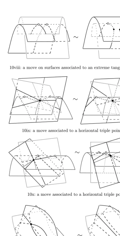
, ifrpasses through a critical moment,Srchanges by a move in Figure 10.

Each move in Figure 10 denotes 2 symmetric moves since the surfacesSrare

symmetric in S1

z under t7!tþ". The following claim will be proved using

bifurcation diagrams of codimension 2 singularities of link diagrams, see Lemma 4.4.

LEMMA5.5.

(a) Suppose that a family of loops fLsg, s2½%1;1&, in the space SL of all links K'V transversally intersects the subspace !ð2Þ _{at s¼0. Then the diagram} surfaceDSðLsÞchanges near0by a move in Figure 10i–x.

(b)If a family of loopsfLsg,s2½%1;1&, in the spaceSLhas a simple tangency with

! ats¼0, thenDSðLsÞchanges near0 by the move in Figure 10xi.

Sketch: The pictures in Figure 10 are obtained from the corresponding pictures in Figure 8. For instance, in Figure 8iii the canonical loop CLðK%"Þ meets 3

subspaces! ;! ;! . Therefore the surface DSðK%"Þ has three distinguished

points: a hanging vertex, a tangent vertex and a critical one as in Figure 10iii. Right after the move when all three points pass through each other, the surface DSðK_þ"Þhas 4 interesting points: three have the previous types, the new one is a

triple vertex. This situation agrees with 4 intersections of CLðKþ"Þ with

codimension 1 subspaces in Figure 8iii. The remaining cases are absolutely analogous.

LEMMA5.6.

(a) For any generic surface S, there is a generic loop L of links such that the diagram surfaceDSðLÞcoincides withS.

(b)For any equivalence of surfaces fSr'Axz#St1g, there is a generic homotopy of loopsfLrgsuch thatDSðLrÞ ¼Sr,r2½0;1&.

Lemma 5.5 and Definition 3.10 of a generic homotopy imply Lemma 5.7. LEMMA5.7. Any generic homotopy of loopsfLsg,s2½0;1&in the spaceSL provides an equivalencefDSðLsÞg of diagram surfaces.

LEMMA5.8. Let L0; L1 be generic loops of links. IfDSðL0ÞandDSðL1Þare

equivalent in the sense of Definition 5.4, thenL0andL1are generically homotopic.

PROOF. Any equivalence of diagram surfaces gives rise to a smooth family of loopsfLrgby Lemma 5.6b. The constructed familyfLrgis a generic homotopy

since all moves in Figure 10 correspond to singularities in the sense of

Definition 3.4. !

By Lemmas 5.7 and 5.8 the classification of generic links reduces to the equivalence problem for their diagram surfaces.

PROPOSITION5.9. Generic links K0; K1 are generically equivalent if and

only if the diagram surfaces DSðK0Þ;DSðK1Þ are equivalent in the sense of

Definition 5.4.

The isotopy class of a link can be easily reconstructed from its plane diagram, hence from its diagram surface with labels. Formally, one has the following.

LEMMA5.10. Suppose that the diagram surfaceDSðKÞof a generic linkKis given, butKis unknown. Then one can reconstruct the isotopy class of K'V.

6. The trace graph of a link as a link invariant.

6.1. The trace graph of a link and generic trace graphs.

Here the classification of links K'V will be reduced to their trace graphs. DEFINITION6.1. LetS'Axz#S1t be the diagram surface of a loop of links.

Thetrace graphTGðSÞis the self-intersection of S, i.e. a finite graph embedded intoAxz#S1t. Thetrace graphTGðKÞof a linkKis the trace graph of its diagram

DEFINITION6.2. A finite graph G'Axz#S1t is generic if Conditions (i)–

(ii) hold.

(i) Conditions ontrace arcsandvertices.

, the graphGconsists of finitely manytrace arcs, which are monotonic arcs with respect to the orthogonal projectionprz:G!S1z;

, any endpoint of a trace arc ofGhas either degree 1 (ahangingvertex ) or degree 2 (acritical vertex );

, the critical vertices ofGcoincide with the critical points ofprz:G!S1z;

, trace arcs ofGintersect transversally attriple vertices ( ); , the critical points of prz:G!S1t are calledtangent vertices( ).

(ii) Conditions onlabels.

, each trace arc ofGis labelled with alabel ðqisjÞas in Definition 4.2;

, undert7!tþ"the graphGmaps to its image under the symmetry inS1

z;

, under the time shiftt7!tþ"each labelðqisjÞreverses toðsjqiÞ;

, every triple vertex v2G is labelled with a triplet ðqisjÞ, ðsjrkÞ, ðqirkÞ

consisting of the labels associated to the trace arcs passing throughv; , each hanging vertex is labelled with the label of the corresponding trace

arc;

, for any i and q¼1;+ + +; ni, there are exactly two hanging vertices of G

labelled withððqþ1Þi; qiÞand ðqi;ðqþ1ÞiÞ, respectively;

, at every critical vertex of G the labels of trace arcs may transform as follows: eitherðqisjÞ$ðqi;ðs-1ÞjÞorðqisjÞ$ððq-1Þi; sjÞ.

A trace arc of a generic graph may consist of several edges in the usual sense. LEMMA6.3.

(a) For any generic surface S, the trace graph TGðSÞ is generic in the sense of Definition 6.2. So the trace graphTGðKÞof a generic linkK is generic.

PROOF. Conditions (i)–(v) of Definition 5.2 imply Conditions (i)–(ii) of

Definition 6.2. !

DEFINITION6.4. A smooth family of trace graphsfGsg, s2½0;1&, is called

anequivalence if there are finitely many critical momentss1;+ + +; sk2½0;1& such

that

, for all non-critical moments s =2 fs1;+ + +; skg, the trace graphs Gs are

generic;

The moves in Figure 11 should be considered locally, i.e. the diagrams do not change outside the pictures. Various mirror images of the moves are also possible. Moreover, some labelssþ1can be replaced bys%1and vice versa. Trace graphs are symmetric undert7!tþ", i.e. each move in Figure 11 denotes two symmetric moves. The most non-trivial moves aretetrahedralmoves 11i andtrihedralmoves 11xi. Their geometric interpretation at the level of links is shown in Figure 12.

Notice that both moves in Figure 11i can be realized for links and closed braids. In general a tetrahedral move corresponds to a link or a braid with a horizontal quadrisecant. Geometrically two arcs intersect a wide band bounded by another two arcs. Under a tetrahedral move, the two intersection points swap their heights as in Figure 12. The first picture of Figure 11i applies when the intermediate oriented arcs go together from one side of the band to another like ". The second picture means that the arcs are antiparallel as in the British rail mark #. It is easier to understand Lemma 6.5 first for knots, when the indices

i; j¼1 can be missed.

LEMMA6.5.

(a)For a generic trace graphGsuch thatGTðAxz#f0gÞare crossings of a general diagram, there is a generic surfaceSsuch thatTGðSÞ ¼G.

(b)For any equivalence of trace graphsfGrg, there is an equivalence of surfacesSr withTGðSrÞ ¼Gr,r2½0;1&.

PROOF.

(a) Consider a vertical sectionPt¼GTðAxz#ftgÞnot containing vertices ofG.

Then Pt is a finite set of points with labels ðqisjÞ, where i; j2 f1;+ + +; mg, see

Definition 5.2. The points inPt will play the role of crossings of sections ofS.

The labelled set Pt defines the Gauss diagram GDt as follows, see

Definition 2.7. Take Fm_i¼1S1

i, split each circle S1i into ni arcs and number them

by1;+ + +; niaccording to the orientation. We mark several points in theq-th arc of S1

i in a 1-1 correspondence and the same order with the points of Pt projected

So each point ofPtgives 2 marked points inFmi¼1Si1, labelled withðqisjÞand

ðsjqiÞ. Connect them by a chord and get the Gauss diagramGDt. The zero Gauss

diagram GD0 is realizable by the given general diagram. Hence all Gauss diagrams GDt give rise to a family of diagrams Dt, i.e. to a surface S¼

S

ðDt#ftgÞ.

(b) Apply the construction from (a) to each trace graphGr,r2½0;1&. !

PROPOSITION6.6.

(a)Trace graphsTGðS0Þ;TGðS1Þof generic surfaces are equivalent in the sense of

Definition 6.4 if and only if the surfaces S0; S1 are equivalent in the sense of

Definition 5.4.

(b)Generic surfacesS0; S1are equivalent in the sense of Definition 5.4 if and only

ifTGðS0Þ;TGðS1Þare equivalent in the sense of Definition 6.4.

PROOF. (a), (b) Any equivalence fSrg of surfaces gives rise to the

equivalenceTGðSrÞ of trace graphs. Any equivalence of trace graphs gives rise

to a smooth family of diagram surfacesfSrgby Lemma 6.5b. The familyfSrgis an

equivalence of diagram surfaces since the moves in Figure 11 are restrictions of

the moves in Figure 10. !

Theorem 1.4 directly follows from Propositions 3.8, 3.12, 5.9 and 6.6. LEMMA6.7. Suppose that the trace graphG¼TGðKÞof a generic linkKis given, butKis unknown. Then one can construct a generic linkK0equivalent toK.

PROOF. Lemma 6.5a provides a generic surface S such that TGðSÞ ¼G. Due to labels of trace arcs, the sectionD0¼STðAxz#f0gÞgives rise to a link K0_{'V with pr}

xzðK0Þ ¼D0. The link K0 can be assumed to be generic by

Proposition 3.8a and is equivalent to K since K and K0 have the same Gauss

diagram. !

6.2. Combinatorial construction of a trace graph.

LEMMA6.8. Let K'V be a link with 2e extrema of the projection prz: K!S1

z andlcrossings in the diagramprxzðKÞ. Let the extrema and intersection points fromKTðDxy#fz¼ -1gÞdivideKintonarcs monotonic with respect to

prz. ThenKis isotopic inV to a linkK0such thatTGðK0Þcontains2lðn%2Þtriple vertices,4ðn%e%1Þecritical vertices and2ehanging vertices.

PROOF. Take a generic link K0 smoothly equivalent to K and having an isotopic plane diagram. We splitK0 _{by horizontal planes into several horizontal}