69thInternational Astronautical Congress (IAC), Bremen, Germany, 1-5 October 2018.
IAC–18–C1.8.5x46264
AN
INTRUSIVE
POLYNOMIAL
ALGEBRA
MULTIPLE
SHOOTING
APPROACH TO THE
SOLUTION OF
OPTIMAL
CONTROL
PROBLEMS
Cristian Grecoa*, Marilena Di Carloa, Massimiliano Vasilea, Richard Epenoyb
aMechanical and Aerospace Department, University of Strathclyde, 75 Montrose Street, Glasgow, United Kingdom
G1 1XJ,{c.greco , marilena.dicarlo , massimiliano.vasile}@strath.ac.uk
b Centre National d’Etudes Spatiales (CNES), 18 Avenue Edouard Belin, Toulouse, France 31401,
*Corresponding author
Abstract
This paper proposes an approach to the solution of optimal control problems under uncertainty, that extends the clas-sical direct multiple shooting transcription to account for random variables defined on extended sets. The proposed approach employs a Generalised Intrusive Polynomial Expansion to model and propagate uncertainty. The develop-ment of a generalised framework for a direct multiple shooting transcription of the optimal control problem starts with the discretisation of the time domain in sub-segments. At the beginning of each segment, the state spatial distribution is modelled with a multivariate polynomial and then propagated to the sub-interval final time. Continuity conditions are implicitly imposed at the boundary of two adjacent segments, a critical operation because it requires the continuity of two extended sets. The Intrusive Polynomial Algebra aNd Multiple shooting Approach (IPANeMA) developed in this paper can handle optimal control problems under a wide range of uncertainty models, e.g. nonparametric, ex-pensive to sample, and imprecise probability distributions. In this paper, the approach is applied to the design of a low-thrust trajectory to a Near-Earth Object with uncertain initial conditions.
Keywords: optimal control under uncertainty; robust control; generalised multiple shooting; intrusive polynomial algebra; low-thrust trajectory optimisation.
1. Introduction
Optimal control problems aim at finding the optimal control law for a single trajectory evolving in a determin-istic nonlinear system. Hence, the resulting control is valid only for the computed reference trajectory. How-ever, in real-life applications, perfect compliance to the reference trajectory is impossible to achieve as uncer-tainty always affects the system; unceruncer-tainty is due to both imperfect state knowledge and to unknown model parameters. Furthermore, for nonlinear systems and large time-scales, even small deviations from a pointwise tra-jectory can lead to significant differences as the system evolves over time. In space applications, low-thrust mis-sions are rather sensitive to trajectory deviations. In-deed, due to the limited control authority, long periods of maximum thrust are required to build up the nominal orbital changes. If possible uncertainty is not taken into account during the stages of trajectory design, this may leave no room for compensation maneuvers. One com-mon cause of trajectory deviation in low-thrust trajecto-ries is missed-thrust due to sub-systems partial failure or external causes, like experienced by Dawn and Hayabusa missions.
To compensate for possible deviations, currently the practical solution is to consider propellant margins and enforced coasting arcs in the reference trajectory design [9]. Several research works developed methods to deal with an optimal control formulation which models un-certainty directly. Methods based on model predictive control or closed-loop formulations takes into account di-rectly correction terms based on possible deviations from the desired trajectory [11][6]. A method based on Taylor polynomials algebra has been developed to deal with un-certain boundary conditions around a reference trajectory [5]. In addition, stochastic differential dynamic program-ming has been applied to space trajectory optimisation with uncertainty with an expected value formulation [8]. The common baseline of these works is the presence of a desired reference trajectory and undesired deviations from it. This problem statement can be either formu-lated implicitly, by working with expected valued objec-tive and constraints, or explicitly, by trying to compen-sate the trajectory deviations. Furthermore, often these techniques can deal only with simple families of proba-bility density distributions to represent uncertainty.
phrased under a more general probabilistic framework. Specifically, the premise of a reference trajectory is aban-doned in favor of an extended uncertainty set representa-tion. Each sample within the uncertainty set is a fully ad-missible pointwise trajectory with associated probability density. Aiming at a probabilistic framework, the objec-tive function and constraint formulation are framed ac-cordingly, since an expected value formulation would re-sult too limited. From here, the goal is to compute control profiles able to optimally steer the uncertain region to a final target set, while minimising the modified objective function. The developed tool is a generalised multiple shooting for the optimal control problem transcription, coupled with intrusive polynomial algebra for the uncer-tainty propagation.
The paper is structured as follows. Section 2 in-troduces the formulation of the addressed optimal con-trol problem under uncertainty. Section 3 presents the main development, first introducing the intrusive poly-nomial algebra propagation, and then integrating it with the novel generalised multiple shooting framework using an expectation formulation for the objective function and constraints. Within this framework, a specific approach is proposed based on polynomial reinitialisation and suc-cessive sampling. The developed tool is then applied to the optimisation of a low-thrust rendezvous trajectory to a Near-Earth Object in Section 4. Finally, Section 5 con-cludes the paper with the final remarks.
2. Optimal Control under Uncertainty
Generally, the deterministic optimal control problem statement is formulated as follows:
min u(t)∈UJ
s.t. x˙ =f(t,x,u,d)
g(t,x,u,d)∈G
ψ(t0,x0, tf,xf)∈Ψ
[1]
The objective functionJcan be in Bolza form in the most general case, i.e. with both end-cost and integral terms, while both pathgand boundaryψconstraints could be imposed. A set inclusion formulation has been used to describe simultaneously both the admissible cases of equality and inequality constraints. This framework is suitable for a single trajectory optimisation.
When uncertainties and random factors come into play, a set of admissible trajectories is associated to a single control. For this situation, the framework above results too limited. The main challenge addressed in this section is the formulation of a general optimal control problem of a dynamical system under uncertainty.
The general uncertainty vector is denoted asZwith probability density distributionp(ξ). Usually, it models
possible uncertainty affecting the initial state and model parameters. As a result, the state and model param-eters become random variables themselves X=X(Z)
andD=D(Z). The lower case lettersξ, xandd de-note an admissible realisation. On the other hand, the control variables will be treated as completely determin-istic input since possible disturbances on the control can be modelled in the dynamics as a multiplicative noise in-corporated inZ.
The dynamical equations induce the state density dis-tribution to evolve over timep(x). In the general nonlin-ear case, computing directly its evolution is an ambitious, and when possible laborious, task. Therefore, this prob-lem is often tackled with sampling techniques. Indeed, the dynamical equations can be used directly as a map from the state and parameter sample space at a given time to the state sample space at another time. The distribu-tion at the time of interest is then reconstructed according to the sample responses, usually by fitting a parametric (possibly discrete) distribution.
In the transition from the deterministic to the uncer-tain setting, the main divergence lies in the definition of objective functions and constraints depending on random variables. Specifically, since the random variable state affects their value, generally they turn out to be random variables themselves. How to formulate an objective or constraint on a random variable is a design choice that directly affects the interpretation and result of the optimi-sation process. Common choices in stochastic program-ming are to impose so-called objective or constraintsin expected value orin probability[2]. In order to have a single notation, we will write both the possible formu-lations in expectation form with the auxiliary function φ. The expectation formulation is flexible as it allows to define a variety of different quantities just selecting the appropriate function. From here, depending on the quantity of interest, the expectation can be minimised or constrained. Specifically for the constraints, the set of acceptable constraint valuesΦfor the inclusion relation-ship should be defined accordingly.
It is worth describing in detail how the expectation formulation encloses common cases of objective or con-straints forms:
• in expected value, for which the function φis the mapping between the trajectory realisation and the quantity of interest. As an example, the expected value of the final stateXf can be constrained to be equal to a target statexf. In this case, the auxiliary function is the identity mapping of the final state
φψ(tf,Xf) =Xf , [2]
resulting in the constraint formulation
69thInternational Astronautical Congress (IAC), Bremen, Germany, 1-5 October 2018.
• in probability, for which the indicator function of a particular event should be employed. For example, we can ask the final state to reach a target regionA with probability larger than or equal to1−α. The auxiliary function is defined as
φψ(tf,Xf) =IA(Xf), [4]
where
IA(Xf =xf) =
(
1 if xf ∈A
0 if xf 6∈A.
[5]
From here, the constraint is formulated as
P(Xf ∈A) =E[IA(Xf)]∈Φψ= [1−α,1].
[6]
• according to higher order moments, for which a spe-cificφand acceptable setΦare selected accorginly.
Among the possible choices, the specific form to min-imise or constraint is a design decision, which translates the question”what do we want to optimise?”. Generally, different design choices lead to different optimisation re-sults.
Given these premises, the optimal control under un-certainty to be tackled in this paper is formulated as
min u(t)∈UE[φJ]
s.t. X˙ =f(t,X,u,D)
E[φg(t,X,u,D)]∈Φg
E[φψ(t0,X0, tf,Xf)]∈Φψ,
[7]
in a comparable way to the classical deterministic opti-mal control problem. The objective auxiliary function φJmay depend on all the random variables when in the Bolza form. Nonetheless, its dependencies have not been written explicitly for conciseness of notation. Clearly, fully deterministic objective and constraints are still al-lowed. In that case, the corresponding function would fall back to Equation (1) notation. One common example is the case of the objective function only depending on the deterministic control.
This paper considers the case of deterministic dynam-ics affected by epistemic uncertainty, but with no intrin-sic stochastic terms. Hence, for a fixed uncertain sample
ξ∈Ωξ, the resulting trajectoryx(t)is deterministic.
In general, an optimal control problem is infinite di-mensional with no closed form solution. This implies that a finite dimensional approximation is required to practically compute a solution with a numerical solver. Transcription methods are schemes which convert a dy-namical optimal control problem into static constrained optimisation one, which is possible to solve with well-established numerical routines, e.g. NLP solvers. The
next section will introduce a general transcription frame-work for optimal control problems with uncertainty in the form of Equation (7).
3. Generalised Direct Multiple Shooting
In the family of transcription techniques, direct meth-ods aim at finding a sequence of control profiles which progressively decrease both the objective function and the constraint’s violation. Within direct methods, the deterministic multiple shooting works by discretising the independent variable interval into ni sub-segments [ti, ti+1], which are then handled as independent. As a consequence, the state xi at the beginning of each ment has to be treated as free variable. Within a seg-ment, the control is parameterised using a functional form with free parametersβi, such that the control pro-file has the finite-dimensional representation ui(t) =
Ui(t,βi). Once these free variable are set by the optimi-sation solver, each statexi is integrated fromti toti+1.
Continuity constraints are added at the boundary of two adjacent segments to ensure continuity of the final solu-tion.
However, when uncertainties are introduced, this pointwise method is not sufficient anymore. This section introduces a generalised shooting framework to deal with potential uncertainty in the initial conditions and dynam-ical model under general form objective and constraints as in Equation (7). A generalised intrusive polynomial expansion approach is used to represent the state variable evolution as function of the uncertain variables in a finite-dimensional space [7]. The resulting approach is named IPANeMA (Intrusive Polynomial Algebra aNd Multiple shooting Approach) for short.
3.1 Intrusive polynomial algebra propagation
The initial uncertain state sample domain Ωx0,
induced by the random variable Z, is bounded by a q-degree nξ-variables polynomial representation
PX0 ∈Tq,nξ, where Tq,nξ is the resulting polynomial
space. Since we are interested in the time evolution of this region, the polynomials approximating the state vec-tor are function of all thenξrandom variables involved:
PX(t) = N
X
j=1
αj(t)Pj(ξ)
PX(t0) =PX0 ,
[8]
whereN = nξ+q
q
is the algebra dimension of the result-ing functional spaceTq,nξ, andPjone of its multivariate
In this functional space, a set of algebraic operations between polynomials can be defined. Denoting with V andZ the multivariate polynomial approximations in Tq,nξofvandz, the algebraic operation⊕={+,−,·, /}
between real-valued functions has its correspondent⊗in the polynomial space:
v(ξ)⊕w(ξ)∼V(ξ)⊗W(ξ)∈Tq,nξ . [9]
The result of the addition (or equivalently subtraction) of two elements ofTq,nξ is still an element of the same
functional space. On the other hand, the result of mul-tiplication needs to be truncated to restore the orderq. Multiplication of two polynomials is an expensive opera-tion, hence the approach used in this analysis will rely on a monomial basis, which guarantees lower compu-tational costs. A composition rule is defined to handle division and other elementary functions such as trigono-metric functions, exponents, logarithms, etc. These poly-nomial operations are implemented using the C++ over-loading operator within the Strathclyde Mechanical and Aerospace Research Toolbox for Uncertainty Quantifica-tion (SMART-UQ) [7].
Given this set of operations, any integrator for the propagation of ordinary differential equations can be eas-ily templated to work with generalised polynomial ex-pansions. This feature enables to propagate the initial hyper-region PX0 through the dynamical system
con-straints in Equation (7).
The uncertain model parameters are handled equiva-lently. The parameter sample domainΩd, induced by the random variableZ, is bounded by a constant multivariate polynomialPD ∈ Tq,nξ, which is composed inPX(t)
through the dynamical operations.
3.2 Multiple shooting framework
Intrusive polynomial algebra could be used directly to propagatePX0, the initial uncertain region, through
the dynamics to obtain the final regionPXf. The latter
polynomial mapping could then be used to compute the objective function and the constraints (see section 3.3) to complete a loop of the optimisation process. This scheme can be seen as a generalised single shooting transcription method.
Despite its simplicity, this polynomial algebra-assisted single-shooting suffers severely from the renowned curse of dimensionality. Indeed, intrusive polynomial algebra scales badly with increasing number of uncertain variables, precisely as(nξ +q)!/(nξ!q! ). Hence, the cost of each algebraic operation involved in the numerical propagation grows dramatically.
When the uncertainties affect the system evolution se-quentially (e.g. multi-phase trajectories, discretised con-trol with disturbances, etc.), this issue can be mitigated
adopting a multiple shooting scheme. In this develop-ment, we will consider the uncertain vector to be com-posed of uncertain initial conditions and model parame-tersZ= [X0,D], and consequently an admissible
reali-sation isξ= [x0,d]. In particular, the uncertain
parame-ter vector is partitioned as D= [D0,D1, . . . ,Di, . . .], such that the parameters Di affect the system only in the discretised interval [ti, ti+1]. From here, the goal is to develop a transcription method such that each sub-segment can be treated independently, and consequently the algebra dimension in the i-th segment reduces to nξi=ns+di, namely the number of the uncertain state
variablesX(ti)at the beginning of the segment and the number of uncertain parametersDiaffecting the system evolution fort∈[ti, ti+1]. With this partition, the accu-mulation of uncertainties is avoided.
If this goal is achieved, each segment can be treated as a single shooting where the polynomial representation of the initial conditionP(Xg)
i attiis propagated toP
(p) Xi+1at
ti+1under the effect of uncertain parametersDionly.
3.2.1 Reinitialisation Approach
The main difficulty of the proposed discretisation arises from the necessity to impose continuity conditions between two hyper-dimensional sets at the boundary of two adjacent segments. For polynomial algebra, this con-tinuity requirement could be translated into a reinitial-isation approach: the propagated polynomial represen-tationP(Xp)
i+1, function ofXi andDi, is reinitialised to
the polynomialP(Xg)
i+1, initially function ofXi+1 only.
Indeed, it is worth stressing that the terms interacting with Di+1 arise only during the propagation, i.e. for
t∈(ti+1, ti+2].
However, in general, it is not possible to fully de-scribe a multivariate polynomial with another polynomial of smaller number of (initial) variables and same degree. To overcome this intrinsic issue, the reinitalised polyno-mial will be constructed to bound the propagated one. In particular, the propagation phase is carried out as follows:
1. Initialisei= 0,P(Xg)
i =PX0;
2. Propagate uncertainty regionP(Xg)
i attitoP
(p) Xi+1at
ti+1through intrusive polynomial algebra;
3. Compute lowerXLi+1and upper XUi+1
polyno-mial ranges ofP(Xp) i+1;
4. Reinitialise uncertainty regionP(Xg)
i+1as hyper-box
with rangeXLi+1andXUi+1;
5. Updatei=i+ 1and repeat steps 2-5 whilei < ni
69thInternational Astronautical Congress (IAC), Bremen, Germany, 1-5 October 2018.
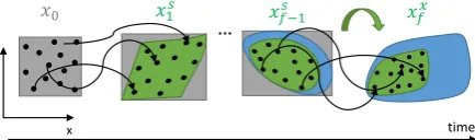
propagating larger regions than strictly needed. Graphi-cally, this procedure can be visualised as in Figure 1 for a two-dimensional example.
𝑋0𝑔 𝑋1𝑝 𝑋1𝑔
x y
x y
xL
xU 𝑓(𝑡, 𝑥, 𝑢, 𝑑1)
…
𝑋𝑓𝑝
time
[image:5.595.313.530.96.160.2]𝑋𝑓−1𝑝 𝑋𝑓−1𝑔
Fig. 1: Graphical sketch of intrusive polynomial propa-gation approach for the generalised multiple shooting. The gray boxes represent the reinitalisation hyper-boxes, whereas the blue regions depict the propagated polyno-mials.
The result of this propagation approach is a chain of polynomial surrogates describing the state at timeti+1as
function of the state at timeti and uncertain parameters within the corresponding interval. Therefore, a recursive polynomial surrogate of the final stateXfis available as a function of the initial conditionsX0and all the
uncer-tain parametersD. At this step however, the hyper-box reinitialisation caused the final state surrogate to be an over-estimation of the true final uncertain space in gen-eral.
The routine to recover the actual terminal region is achieved by successive sampling. In the simplest form, the final hyper-region computation algorithm is described as follows:
1. Initialisei= 0
2. Sample the initial uncertain space:
x(is)∈Ωx0
3. Sample thei−uncertain parameter space:
di∈Ωdi
4. Propagate each particle fromtitoti+1with
polyno-mial surrogateP(Xp) i+1: (x(is),di)→xi+1
5. Each response state is scaled within the polynomial input domain using the same ranges XLi+1 and
XUi+1used for polynomial reinitialisation:
xi+1→x (s) i+1
6. Updatei=i+ 1and repeat steps 3-5 whilei < ni (skip step 5 for last iteration)
A graphical depiction of the recovery strategy is plotted in Figure 2.
𝑋0 𝑋1
𝑝 𝑋
1
x y
x y
xL
xU
… 𝑋𝑓−1
𝑝 𝑋
𝑓−1 𝑋𝑓
𝑝
time
𝑥0
x y
…
time
𝑥1𝑠 𝑥𝑓−1𝑠 𝑥𝑓𝑥
Fig. 2: Graphical sketch of the recovery approach for the generalised multiple shooting. The gray boxes represent the reinitialisation hyper-boxes, the blue regions depict the propagated polynomials, while the grey areas sym-bolise the true uncertainty regions reconstructed by the black samples.
It is worth noting that the samples can be propagated at any intermediate time of interest¯t ∈ (ti, ti+1) with-out the need of further discretisation. Trivially, an inter-mediate polynomial can be saved during the propagation phase, and the samples(x(is),di)propagated to¯tthrough it. Hence, the general result of this approach is a surro-gate modelFe¯t : Ωx0×Ωd0:i → R
ns that maps the
un-certain initial conditions and parameters to the state vec-tor at any timet¯. The uncertain parameter spaceΩd0:i
takes into account only the model uncertain parameters
D0:i = [D0, . . . ,Di]which entered the system not later than the time of interest.
With the developed generalised multiple shooting ap-proach, the uncertain space dimensionality is kept as low as possible in each discretisation interval. Further-more, the outer reinitialisation strategy intrinsically im-plies pointwise trajectory continuity. This property re-moves the need of explicit defect constraints and interme-diate free variables in the transcription, hence reducing the dimensionality of the associated constrained optimi-sation problem. The only free variables to be optimised are the control parameters in each sub-segment. Another powerful upside of this method is that the sampling in steps 2-3 is agnostic to the probability distribution na-ture. Therefore, the method is equally suitable for any probability distribution.
The missing bit for a complete transcription scheme for uncertain optimal control problems is the computa-tion of expectacomputa-tions of generic funccomputa-tions as introduced in Section 2.
3.3 Objective and constraint computation
In the problem statement development, the general expectation formulation was chosen to represent a wide class of possible constraints and objective functions. In-deed, the generic functionφis considered a design choice to be selected according to the sought quantity of inter-est. Furthermore, the expectation can be computed at any fixed-time¯t, or even on a time-span of interest.
[image:5.595.68.289.144.215.2]of the surrogate modelFe¯t, approximating the true map-ping, as defined in the previous section:
E[φ(X(¯t))]≈E[φ(Fet¯(Z0:i))]
=
Z
Ωξ 0:i
φ(Fe¯t(ξ0:i))p(ξ0:i)dξ0:i, [10]
where the random variable is defined as
Z0:i= [X0,D0:i], its realisation asξ0:i = [x0,d0:i], and the uncertain domainΩξ0:i= Ωx0×Ωd0:i.
In the general case, this integral has no closed-form solution and numerical techniques shall be ap-plied. Exploiting the inexpensive surrogate map, two main sample-based alternatives can be considered:
• Monte Carlo methods for the estimation of the ex-pectation: the samples in steps 2-3 of the recov-ery strategy shall be drawn according to the un-certain variables propability distributionsp(x0)and
p(d0:i). Then, the expected value can be computed as:
E[φ(Fe¯t(Z0:i))]≈ 1
N
N
X
j=1
φ(Fe¯t(ξ (j)
0:i)); [11]
• Quadrature schemes for the computation of the inte-gral: the samples are chosen according to a quadra-ture scheme with corresponding weightswj, result-ing in the integral approximation
Z
Ωξ 0:i
φ(Fet¯(ξ0:i))p(ξ0:i)dξ0:i≈
N
X
j=1
wjφ(Fet¯(ξ (j) 0:i))p(ξ
(j) 0:i).
[12]
The latter scheme shall be preferred when the probability distribution is complex to sample but rather easy to eval-uate, or when the expectation should be evaluated for a set of different density distributions.
It is worth suggesting that when this approximation is included in a NLP local optimisation solver with finite-difference derivative computation, sampling grids should be kept constant within a major NLP step. Indeed, if the grids are varied between the reference and perturbed propagations, the derivative values would result highly inaccurate, leading the optimiser to compute unreliable descent directions.
Although probability constraints (or equivalently ob-jectives) are an intuitive and general tool to impose condi-tions on random variables, the indicator function discon-tinuity introduces important numerical challenges when coupled with derivative-based optimisers. Indeed, al-though in theory the expectation operator should smooth
the discontinuity, the final constraint is usually com-puted by sample-based numerical approximations (as in eq. (11) or (12)), which cause the constraint response to be piecewise constant with discontinuous jumps. Local derivative-based optimisers cannot cope with such func-tions.
To overcome this numerical issue, the developed tool substitutes the indicator function by a smoother approxi-mation obtained by convolution [2], a general technique to modify the shape of a function according to a smooth-ing function h. To simplify the convolution applica-tion to a scalar funcapplica-tion of scalar variable, the member-ship condition of a sample belonging to a regionAwill be expressed by an auxiliary continuous scalar function ηA:Rns →Rsuch that:
(
|ηA(X=x)|≤1 if x∈A
|ηA(X=x)|>1 if x6∈A.
[13]
Hence, the indicator function previously defined is equiv-alent toIA(X) =I[−1,+1](ηA(X)). Now, for a state re-alisationx, the convolution of the indicator function with a smoothing functionhresults in the function:
I([−r)1,+1](ηA(X=x)) =
Z+∞
−∞
I[−1,+1](y) 1 rh
ηA(x)−y
r
dy
=
Z+1
−1
I[−1,+1](y) 1 rh
ηA(x)−y
r
dy,
[14] with r > 0 a small positive scaling parameter. The integration interval is restricted to the interval[−1,+1]
because of the function ηA definition. The function
h is chosen to result in a proper approximation of the original function. Specifically, h : R → R shall be non-negative, symmetric, with an unique maximum in 0, and it shall integrate to 1. These properties imply
limr→0h(·/r)/r=δ, the Dirac delta. Hence, forr→0
the convolution result tends to the original indicator func-tion [2].
It is worth mentioning that objective and constraints not falling under the expectation formulation are possi-ble. As an example, if we are interested in the final state ending in the target region A, one alternative is to constraint the maximum deviation to be under a set threshold, e.g. max({|ηA(x(j))|:j= 1, . . . , N})≤ρ . Similar objective and constraint functions are rather test case specific and hence not explicitly accounted for, but nonetheless possible in the developed framework.
3.4 Transcribed problem
69thInternational Astronautical Congress (IAC), Bremen, Germany, 1-5 October 2018.
deterministic multiple shooting, the resulting transcribed problem is dense and low-dimensional, as no intermedi-ate stintermedi-ate guesses or explicit continuity constraints have been introduced. Hence, the control parametersβi per each sub-segment are the only free variables.
To avoid a new expensive intrusive polynomial prop-agation each time a free variable vector is set within the optimisation routine, the deterministic control can be ex-panded in polynomial representation as well. Specifi-cally, the control parameters domainΩβican be bounded
by a time-static multivariate polynomial Bi ∈ Tq,nξi, where the number of uncertain variablesnξi should be
increased accordingly. Then, the polynomial control pro-file in each interval follows according to the parameter-control relationshipUi(t) =U
(p)
i (t,Bi), where byU (p) i it is intended the corresponding polynomial operator of Ui. For a fixed value βi ∈ Ωβi, the control
polyno-mial representation reduces to the deterministic control
ui(t) =Ui(t,βi). With this procedure, only one uncer-tainty polynomial propagation is needed, and it can be precomputed before the optimisation cycle.
4. Test case
The developed method is applied to the optimisation of a space trajectory. The goal of the set-up mission is to compute the optimal-fuel rendezvous to the near-Earth asteroid 99942 Apophis (2004 MN4) with a low-thrust
spacecraft departing from the Earth sphere of influence. The initial date of the interplanetary leg is 22/10/2026 for a total time of flight of 628 days. The engine has max-imum thrust ofTmax= 53mN, for a spacecraft initial mass ofm0= 644.3kg. The reference mission employs
an initial excess velocity of magnitudevref∞ = 3.34km/s and azimuth angleαref
∞ = 35.17deg deviation from the
x−axis in the Earth-centered inertial reference frame. As this case is meant at assessing the suitability and performance of the developed method to preliminary de-sign of robust space trajectories, a few simplifying as-sumptions will be used. Namely, only the Sun pull is considered as gravitational force, and only the planar tra-jectory is studied.
The spacecraft planar motion is described in equinoc-tial coordinate system for the in-plane coordinates [3]:
a
P1=esin (Ω +ω)
P2=ecos (Ω +ω).
[15]
The governing equations are expressed in the Gauss’ planetary form in a radial-transverse reference frame. The fast angular variableL, i.e. the true longitude, can be used as independent variable to replace the time evolu-tion. Under the enforced assumption of a low-thrust con-trol magnitude significantly smaller than the local
gravi-tational force, the resulting system of equations is [13]:
da dL=
2a3B2 µ
"
P2sinL−P1cosL
Φ2(L) fR+
1 Φ(L)fT
#
dP1 dL =
B4a2 µ
"
− cosL
Φ2(L)fR+
P1+ sinL Φ3(L) +
sinL Φ2(L)
!
fT
#
dP2 dL =
B4a2 µ
"
+ sinL
Φ2(L)fR+
P2+ cosL Φ3(L) +
cosL Φ2(L)
!
fT
# ,
[16]
where B =p(1−P2
1 −P22) and Φ(L) = 1 +P1sinL+P2cosL. The radial and
transverse control components are controlled in terms of acceleration magnitude and azimuth angle:
f = fR fT = sinα cosα . [17]
For the deterministic reference case, the terminal con-straint is imposed by requiring the matching of the space-craft final state with Apophis in equinoctial elements at the time of arrival. The optimal-fuel objective to min-imise is the trajectory∆V. The first guess for the ref-erence trajectory has been generated by the deterministic single-shooting tool FABLE (Fast Analytical Boundary-value Low-thrust Estimator) [4], which transcribes the optimal control problem into a sequence of coast and constant thrust arcs. In FABLE, the dynamics in Equa-tion (16) is analytically propagated using a first-order ex-pansion in the perturbing control acceleration [13]. The resulting objective value is∆V = 2.0318km/s.
In the following, a fictitious scenario is considered to introduce uncertainty. Telemetry has reported a partial failure in the interplanetary orbit injection phase, but ac-curate information about the new spacecraft state after failure is not available yet. From the partial data, the un-certainty has been traced back to the injection velocity. Specifically, the azimuth angle error∆αref
∞ is modelled with zero-mean normal distribution about the reference value with1σ = 0.25deg, while the magnitude veloc-ity error ∆vref
∞ is modelled with a zero-mean reversed Gaussian tail distribution with1σ= 25m/s, where only negatives values are admissible. The uncertain vector, composed asZ= [∆αref
1.032 1.034 1.036 1.038
a [au]
-0.071 -0.07 -0.069 -0.068 -0.067
P1 [rad]
1.032 1.034 1.036 1.038
a [au]
0.07 0.072 0.074
P2 [rad]
Samples Expected Value 1 Ellipsoid
-0.071 -0.07 -0.069 -0.068 -0.067
P1 [rad]
0.07 0.072 0.074
[image:8.595.64.287.93.408.2]P2 [rad]
Fig. 3: Initial set of uncertainty in equinoctial elements as a result of uncertainty in the excess velocity with su-perimposed the expected value and1σellipsoid resulting from to the sample distribution.
To counteract this partial failure, it has been decided to compute a modified control profile able to steer the initial uncertain region into a target zone around the asteroid state. With this approach, the goal is to limit the required correction manoeuvres, either in-flight or at arrival, when accurate measurements will be available.
This optimal control problem under uncertainty is for-mulated by substituting the final boundary condition with a probability constraint. Specifically, the probability of the final uncertain state to belong to a target ellipsoidT is required to be above a given threshold. The probabil-ity constraint is defined thanks to the auxiliary positive continuous function that, for a given state realisationx, is defined as
ηT(X=x) = (x−µ)TM(x−µ) =
(
≤1 if x∈T >1 if x6∈T ,
[18] where µ is the target ellipsoid center, i.e. the aster-oid state at the time at arrival, while M is defined such that its eigenvectors are the ellipsoid principal axes and its eigenvalues are the reciprocals of the semi-axes
squared. In this test case, M is defined as symmet-ric, while its eigenvalues follow from the set semi-axes
10−3·[2.2au,2.0rad,3.7rad]. The probability
thresh-old has been set to95%.
To solve this optimal control under uncertainty, 5-degree Chebyshev polynomials are employed for the in-trusive propagation, which have been already used in aerospace applications because of their superior global convergence properties [1, 10]. As regards the tran-scription, the following settings are used: 6 discretisa-tion intervals; piecewise constant control; 200 samples for Monte Carlo approximation of Equation (10); bi-quadratic function
h(z) = 15(1−z2)2I[−1,+1]/16
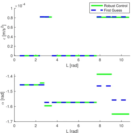
for the convolution operator [2]. The resulting control profile and the first guess are shown in Figure 4.
0 2 4 6 8 10
L [rad] 0
0.2 0.4 0.6 0.8 1
[m/s
2]
10-4 Robust Control
First Guess
0 2 4 6 8 10
L [rad] -1.7
-1.6 -1.5 -1.4
[rad]
Fig. 4: Optimised robust control profile components ver-sus first guess control.
While the thrust magnitude is essentially unaltered, implying a robust ∆V objective value, the thrust angle changed significantly to steer the final region within the required target ellipsoid. The optimisation routine fin-ished with a probability of95.3%associated to the final state arriving within the target region, improving the tra-jectory reliability from the value of22.7%associated to the first guess control.
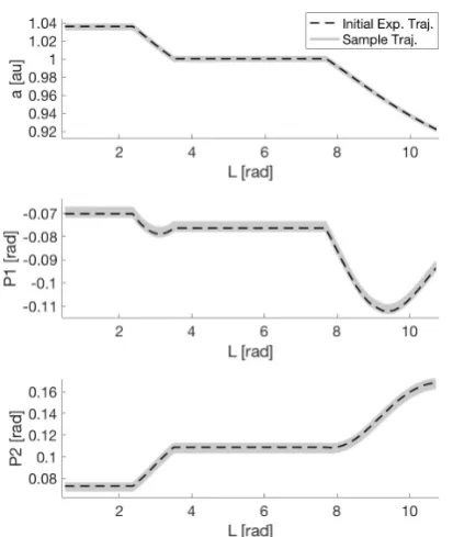
The resulting L-evolution of the uncertain region is shown in Figure 5, where the trajectory of the initial ex-pected value is highlighted with a black dotted line.
[image:8.595.309.529.313.535.2]69thInternational Astronautical Congress (IAC), Bremen, Germany, 1-5 October 2018.
Fig. 5: Uncertain set evolution as function of indepen-dent variable L. The trajectory of the initial expected value is reported with a black dotted line.
extension of the uncertain region have remained essen-tially unaffected during the dynamics propagation. The reason behind this effect is twofold. First, the equinoctial state variables are integrals of motion of the two body problem, hence only partially affected by the small per-turbative force in a limited time-span. Technically, the dynamical system is not fully controllable because of the limited low-thrust control authority. Second, for the given dynamics and initial uncertain set, it is not possi-ble to make all the possipossi-ble trajectories converge within an arbitrary final region with a single open-loop control profile.
For validation, two key approximations employed in the optimisation routine are checked, namely the surro-gate propagation by intrusive polynomial algebra, and the probability approximation by convolution on a rather small set of samples. For the former,105samples drawn
from the initial distribution are reintegrated with the re-fined control profile, with both the polynomial surrogate and a numerical fourth order Runge-Kutta integrator for comparison. The resulting root-mean-square error is in the order of10−5 per state component, which confirms
that intrusive polynomial algebra produces a satisfactory propagation approximation. As for the latter, the final probability is then computed with the indicator function directly, i.e. without the convolution approximation, on the extended validation set of RK4 propagated samples. The resulting probability is 94.0%, slightly lower than the value obtained in the optimisation loop. This
discrep-0.92 0.921 0.922 0.923 0.924 a [au]
-0.095 -0.094 -0.093 -0.092 -0.091
P1 [rad]
0.919 0.92 0.921 0.922 0.923 0.924 0.925 a [au]
0.164 0.166 0.168 0.17 0.172
P2 [rad]
Samples Target Ellipsoid
-0.095 -0.094 -0.093 -0.092 -0.091 P1 [rad]
0.164 0.166 0.168 0.17 0.172
[image:9.595.71.278.91.336.2]P2 [rad]
Fig. 6: Final set of uncertainty in equinoctial elements sulting from optimised control profile and final target re-gion.
ancy results partly from the convolution approximation, but mainly from the different orders of magnitude of un-certainty samples employed. More uncertain samples can be used in the optimisation loop to improve the solution accuracy. Nonetheless, for the current test case, the ob-tained results are considered highly satisfactory.
[image:9.595.305.531.94.413.2]The reliability percentages associated to different set-tings are summarised in the following table.
Table 1: Probability of final target matching for different settings.
Setting Samples Convolution P(Xf ∈T)
First guess 2·102 Yes 22.7%
Guess validation 105 No 23.3%
Robust solution 2·102 Yes 95.3%
Robust validation 105 No 94.0%
5. Conclusions
the solution of optimal control problems affected by un-certainty.
First, a general problem statement is introduced, which reformulates in expectation the constraints and ob-jective functions affected by uncertainty. Thanks to the intermediate auxiliary function, this general notation is shown to be flexible in describing a variety of formula-tions, e.g. expected value, probability, different statistics, etc.
Then, IPANeMA is presented as tool for the transcrip-tion of the infinite-dimensional optimal control problem under uncertainty into a constrained optimisation possi-ble to solve with a NLP solver. IPANeMA integrates a novel multiple shooting framework with a generalised in-trusive polynomial expansion to represent and propagate uncertainty regions. One approach based on reinitialisa-tion by bounding hyper-boxes is proposed, which reduces the intrusive algebra dimension, and intrinsically handles the continuity conditions between two adjacent segments with no need of additional constraints. A sample-based recovery strategy is employed as the reinitialisation ap-proach requires propagating wider regions than the actual one.
The developed framework is capable of handling both uncertainty in the initial state and in the model param-eters. Furthermore, IPANeMA is suitable to work with a large variety of uncertainty models, hence it is not re-stricted to purely Gaussian, uniform or other basic prob-ability distribution families. Indeed, the sample-based strategy developed naturally suits the approximate com-putation of constraints and objective functions formu-lated in expectation. A specific convolution approach is integrated to deal with numerical complexities in the optimisation loop introduced by the probability formula-tion.
Finally, IPANeMA is successfully applied to the ro-bust optimisation of a low-thrust rendezvous trajectory to the near-Earth asteroid 99942 Apophis. In particular, the found control law steers the initial uncertain region to a target ellipsoid around the asteroid, with a probabilistic constraints satisfied within the required threshold.
As for future developments, the main challenge is to integrate observations within IPANeMA for the compu-tation of an updated control law which takes into account the measurement information. The developed framework seems to suit naturally an interface with a particle filter.
Acknowledgements
This work was partially funded by the European Commission’s H2020 programme, through the H2020-MSCA-ITN-2016 UTOPIAE Marie Curie Innovative Training Network, grant agreement 722734.
References
[1] C. O. Absil, R. Serra, A. Riccardi, and M. Vasile. De-orbiting and re-entry analysis with generalised intrusive polynomial expansions. 67th Interna-tional Astronautical Congress, 2016.
[2] L. Andrieu, G. Cohen, and F. Vzquez-Abad. Stochastic programming with probability con-straints.arXiv preprint arXiv:0708.0281, 2007.
[3] R. Broucke and P. J. Cefola. On the equinoctial or-bit elements. Celestial Mechanics, 5(3):303–310, 1972.
[4] M. Di Carlo, J. M. Romero Martin, and
M. Vasile. CAMELOT: Computational-Analytical Multi-fidElity Low-thrust Optimisation Toolbox. CEAS Space Journal, 10:25–36, 2018.
[5] P. Di Lizia, R. Armellin, F. Bernelli-Zazzera, and M. Berz. High order optimal control of space tra-jectories with uncertain boundary conditions. Acta Astronautica, 93:217–229, 2014.
[6] E.D. Gustafson. Stochastic Optimal Control of Spacecraft. PhD thesis, The University of Michi-gan, 2010.
[7] C. Ortega, A. Riccardi, M. Vasile, and C. Tardioli. SMART-UQ: Uncertainty Quantification Toolbox for Generalised Intrusive and non Intrusive Polyno-mial Algebra. In6th International Conference on Astrodynamics Tools and Techniques, 2016.
[8] N. Ozaki, S. Campagnola, C.H. Yam, and R. Fu-nase. Differential dynamic programming approach for robust-optimal low-thrust trajectory design con-sidering uncertainty. In25th International Sympo-sium on Space Flight Dynamics, 2015.
[9] M. D. Rayman and S.N. Williams. Design of the first interplanetary solar electric propulsion mis-sion. Journal of Spacecraft and Rockets, 3:589– 595, 2002.
[10] A. Riccardi, C. Tardioli, and M. Vasile. An in-trusive approach to uncertainty propagation in or-bital mechanics based on Tchebycheff polynomial algebra.Advances in Astronautical Sciences, pages 707–722, 2015.
69thInternational Astronautical Congress (IAC), Bremen, Germany, 1-5 October 2018.
[12] D. Wassel, F. Wolff, J. Vogelsang, and C. Buskens. The ESA NLP-Solver WORHP - Recent Devel-opments and Applications. In Modeling and Op-timization in Space Engineering, pages 85–110. Springer, New York, 2013.