Creep-fatigue and cyclically enhanced creep mechanisms in aluminium based metal matrix composites

M

AN

US

CR

IP

T

AC

CE

PT

ED

Creep fatigue assessment procedure adopted for

crack initiation assessment.

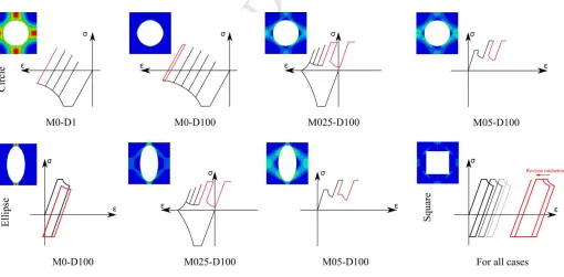
Reference transition hysteresis loops for the three cross-section

studied.

M

AN

US

CR

IP

T

AC

CE

PT

ED

1

Creep-fatigue and cyclically enhanced creep mechanisms in aluminium based Metal

Matrix Composites

Dario Giugliano 1, Daniele Barbera2, Haofeng Chen1*, Nak-Kyun Cho1, Yinghua Liu3

1_{Department of Mechanical & Aerospace Engineering, University of Strathclyde, Glasgow, G1 1XJ, UK} 2_{School of engineering, University of Glasgow, Glasgow, G12 8QQ, UK}

3_{Department of Engineering Mechanics, Tsinghua University, Beijing, 100084, China}

*

Email: [email protected]

Abstract

An aluminium (Al 2024T3) matrix composite reinforced with continuous alumina (Al2O3)fibresis investigated under

tensile off-axis constant macro stress and thermal cyclic loading. The micromechanical approach to modelling and

three different fibre cross-section geometries have been employed. The effect of creep is included by considering

three dwell times at the peak temperature of the thermal loading history. The presence of the hold time gives rise to

different sources of failure such as cyclic enhanced creep and creep ratchetting. These failure mechanisms are

carefully discussed and assessed. The linear matching method framework has been used for the direct evaluation of

the crucial parameters for creep-fatigue crack initiation assessment at the steady cycle. A detailed representation of

the steady-state hysteresis loops is provided by using the strain range partitioning and a method for dealing with

multiaxiality is reported with regard to the algebraic sign of the Mises-Hencky equivalent stress and strain. All the

results obtained have been benchmarked by fully inelastic step-by-step (SBS) analyses. The design of a long fibre

metal matrix composite should consider not only the detrimental effect of their dissimilar coefficient of thermal

expansion, but also the state of stress at the interface between the matrix and fibre.

Keywords: Linear Matching Method (LMM); Cyclic Plasticity; Low Cycle Fatigue (LCF); Creep-Fatigue Interaction; Metal

Matrix Composite (MMC).

1 Introduction

Metal matrix composites (MMCs), are undergoing rapid development to keep up with the requirements of aerospace

and automotive industrial sector applications where minimal weight, and increased efficiency are critical factors

(Cantor et al., 2003). Predicting composite behaviour under hostile and demanding environments due to the combined

action of thermal and mechanical loading, allow for much more effective and reliable use of these complex materials.

When a temperature hold time within the cyclic thermal loading is imposed, a combination of thermal fatigue and

creep damage occur inside the matrix. Creep produces intergranular cavitation damage that is strongly affected by the

hold time’s position within the loading cycle. If the creep dwell starts at the pick of the tensile stress, intergranular

M

AN

US

CR

IP

T

AC

CE

PT

ED

2

of cracks and with continued cyclic loading the cracks propagate through transgranular paths, with surface striations

and wide surface cracks.

In engineering components operating at high temperature, creep lifetime can be significantly reduced when a cyclic

mechanical loading is superimposed in the creep regime. Four types of damage’s interactions can occur i.e. pure

fatigue, transgranular competing, mixed interaction and pure creep (Barbera et al., 2016b), depending on strain range

and dwell time (Hales, 1980; Plumbridge, 1987). A better understanding of the micro material scale is necessary to

ensure that certain types of failure mechanism do not arise, such as low cycle fatigue (LCF) crack initiation,

ratchetting, cyclically enhanced creep or creep ratchetting. This involves the determination of the shakedown limit,

ratchet limit, plastic strain range for LCF assessment, and creep cyclic plasticity interaction (Barbera et al., 2016b;

Giugliano et al., 2017; Giugliano and Chen, 2016). The schematic representation of the stress-strain material response

due to cyclic loading with creep dwell at the tensile peak, as reported in (Barbera et al., 2016b), clarifies the

importance of the aforementioned design limits. Indeed when the load level is below the elastic limit, no plastic strain

occurs at the first cycle and the subsequent creep stress relaxation does not cause any plasticity during the following

unloading and loading phases. Plasticity at the first cycle occurs when the load point is above the elastic limit. Here

different scenarios can take place depending upon the load level i.e. the effect of primary and secondary loads, and

dwell time. If the load level is largely below the shakedown limit and the dwell time is short enough, the stress

relaxation during the subsequent creep hold times is not significant; hence no plastic strain occurs during the

subsequent cycles. The steady-state response is similar to shakedown and the accumulated creep damage is identical

to the monotonic load case. Instead for a higher load level in the shakedown zone but close to the shakedown limit,

creep enhanced plasticity can occur which lead to either cyclically enhanced creep or creep ratchetting (EDF Energy,

2014). Two scenarios are possible when cyclically enhanced creep occur depending upon the magnitude of the

primary and secondary loads. For both cases, a steady-state closed loop response appears either with only creep strain

in loading or with both plastic strain and creep strain in loading. As a closed loop is expected, the inelastic strain in

loading is compensated by the reverse plasticity in unloading. Compared to the monotonic load, more severe

creep-fatigue damage arises. When the inelastic strain in loading is not compensated by the plastic strain in unloading, a

mechanism known as creep ratchetting is expected (Chen et al., 2014). Ratchetting is a cyclic phenomenon, which

result in the progressive accumulation of plastic strain. From Bree (Bree, 1967), it is known that for general

thermomechanical cyclic loading without hold time, if the structure operates in a region of strict or global shakedown

no inelastic strain accumulation occurs. This statement, as discussed previously, becomes imprecise when stress

relaxation due to creep dwell arises. Indeed, if within the shakedown zone, particular conditions in terms of load level

and hold time are satisfied, either cyclically enhanced creep or creep ratchetting occurs.

The effects of pure thermal fatigue with constant off-axis mechanical load (Chen and Ponter, 2005; Giugliano et al.,

2017; Giugliano and Chen, 2016; Jansson et al., 1994; Jansson and Leckie, 1992; Ponter and Leckie, 1998a, b) and

thermo-mechanical fatigue (TMF) with hold time (Barbera et al., 2016a; Bettge et al., 2007; Halford et al., 2000;

M

AN

US

CR

IP

T

AC

CE

PT

ED

3

2011) on MMCs have been under the attention of the authors over the last five years . The aim of this work is to

investigate the impact of three different fibre section geometries i.e. circular section, elliptical

cross-section and square cross-cross-section on the creep-fatigue interaction behaviour of continuous fibre reinforced aluminium

matrix composites (CFAMCs). For the loading conditions investigated, the stress state at the matrix-fibre’s interface,

gives rise to a new ratchetting mechanism which affects the cyclic stress-strain hysteresis loop of CFAMCs. Indeed,

by superimposing a cyclic thermal load with dwell time over an off-axis constant macro stress, a scenario where

mechanical and thermal stresses at the matrix-fibre’s interface act in the opposite direction can occur. In this situation,

the effect of both stress relaxation and residual stress field can lead the structure to experience creep ratchetting with a

total open hysteresis loop (TOL). This work, will explore the damaging effect of this new mechanism which has been

neglected in (Barbera et al., 2016a, b). A great number of numerical simulations are required to study different

geometries, with each being subjected to a variety of loading conditions and dwell times. For this reason the

traditional Abaqus (Abaqus, 2013) incremental finite element approach is not a viable option due to the large

computational cost. In order to perform an accurate and efficient analysis the Linear Matching Method (LMM) is used

in this work, which has been demonstrated to be capable of providing solutions for different classes of problems

(Chen, 2010; Chen et al., 2014; Chen and Ponter, 2010; Giugliano et al., 2017; Giugliano and Chen, 2016; Gorash and

Chen, 2013; Xuanchen Zhu, 2017). Recently the extended LMM Direct Steady Cyclic Analysis (eDSCA) has been

adopted by the authors to perform a preliminary study on the creep and fatigue response of a MMCs unit cell (Barbera

et al., 2016a), further demonstrating the method’s applicability. Although the numerical results presented require

extensive experimental verifications before they can be generally adopted, the features were chosen on the basis of the

reasonableness of their prediction in several cases where they could be anticipated with some confidence (EDF

Energy, 2014).

2 Numerical method

In order to calculate the steady-state cycle response of a structure subjected to an arbitrary cyclic load history, a

numerical procedure based on the minimization process of

( )

1

L

c l

ij l

I

ε

I

=

=

∑

&

has been developed (Chen et al., 2014;

Chen and Ponter, 2006) and further tested (Barbera et al., 2016a; Gorash and Chen, 2013). This function is related to a

class of kinematic admissible strain rate c i j

ε& , defined for a L total number of loading instances. An incremental form

has been proposed for the minimization function as follow:

( )

{

ˆ

( )

( )

}

l l l l l l l

ij ij ij ij l ij l ij

V

I

∆

ε

=

∫

σ ε

∆ −

_



σ

t

+

ρ

t

_



∆

ε

dV

₍₁₎

Where

σ

_ijl is the cyclic stress calculated at load instance “l”, l ij

ε

∆ is the inelastic strain increment, and

σ

ˆ

_ijl

( )

t

_l is the linear elastic stress associated to the cyclic history considering cyclic and constant loading and l

( )

ij tl

M

AN

US

CR

IP

T

AC

CE

PT

ED

4 formulation allows the strain rate history c

i j

ε& to be replaced with a sequence of increments of strain

∆

ε

_ijl , which occur during the load cycle at each time tl. The eDSCA is capable of calculating, by iterative mean, the inelastic strain

increment l ij

ε

∆ , which minimize the function shown in equation (1). A total of K sub-cycles are requested to reach the convergence. Within each k sub-cycle a total of L load increments need to be performed. The residual stress field and inelastic strain increment associated to each load instance l are obtained. At each increment the residual stress and inelastic strain are calculated by the elastic stress and the previous accumulated residual stresses. When the load

instance does not contain a creep dwell, the plastic strain increment

∆

ε

_{ij k, +1}( )t_l ' can be calculated by:

' '

, 1( ) , 1 1 , 1

1

ˆ ( ) ( ) ( )

2 ( ) l

ij k ij l ij k l ij k l

l

t t t t

t

ε σ ρ ρ

µ

+ + − +

∆ =



_

+ + ∆



_

₍₂₎

where notation ( ' ) refers to the deviator component of stresses and µ is the iterative shear modulus (Chen et al.,

2014),

σ

ˆ

_ij is the associated elastic solution,

ρ

_{ij k, +1}

(

t

_l−1

)

is the prior changing residual stress history and

∆

ρ

_{ij k, +1}

( )

t

_l

is the residual stress associated to the inelastic strain increment. If required, the calculated plastic strain is used to

iteratively change the yield stress in the upcoming k+1 sub-cycle, considering the Ramberg-Osgood (RO) (Skelton et

al., 1997) material response. The Ramberg-Osgood model is based on the interpolation of cyclic data at different

strain range at the steady state (saturated cycle). The combination of all these points’ forms the well-known “locus of

the tips” (Hales et al., 2002). This approach allows considering the stabilised loop, at different strain range, for cyclic

hardening or softening materials, however does not consider the evolution of the cyclic response of the structures that

is considered negligible.

In load cases where creep is present, the equivalent creep strain increment∆εc_{is calculated by the following equation}

for the associated dwell time

∆

t

using the Norton-Bailey relation:

1 1 1

( 1) ( )

1 1

( )( 1)

m

c s c

n n

c s

B n t

m σ σ ε σ σ + − − − ∆ − ∆ =

− + (3)

whereB,m and n are the creep constants of the material.

σ

_crepresents the creep flow stress, which is the sum of the

start-of-dwell stress

σ

_s and the residual stress

∆

ρ

_ijccaused by the dwell period. The creep flow stress is then

determined by accurately evaluating the creep strain rate ε_&F _{at the end of the dwell time:}

1

1 1

( 1) 1 1

( 1) ( )

F _n c m n c F c n n

s c c s

B t m t n ε σ σ ε ε

σ σ σ − σ −

M

AN

US

CR

IP

T

AC

CE

PT

ED

5

The remaining part of the procedure calculates the residual stress at each increment through the solution of linear

problems. The residual stress field and the iterative shear modulus obtained are updated for the next cycle k+1 for

each load instance t_lby adopting the linear matching equation;

( )

( )

₍

_{( )}

_{( )}

₎

1

( , )

, ,

ˆ , ,

R y l k

k l k l r

ij l ij l k x t

x t x t

x t x t

σ

µ µ

σ σ ρ

+ =

+ (5)

where

µ

_k

( )

x t

,

_l is the iterative shear modulus at the sub-cycle k for lth load instance. R( , )

y x tl k

σ

is the iterative yield

stress for RO material model or yield stress for the Elastic Perfectly Plastic material model at load instance

t

_l. The

yield stress R( , )

y x tl k

σ

will be replaced by creep flow stress if creep relaxation occurs at the load instance.

( )

,

r ij x tl k

ρ

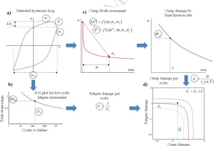
is the sum of the constant residual stress field and all the previous changing residual stresses at different load instances. This procedure is capable of characterizing the whole steady-state cycle calculating both plastic and creep response and considering their combined effects. Once the entire numerical process is converged the creep fatigue endurance can be evaluated. The required key parameters for the assessment can be accurately calculated from the stabilised hysteresis loop by adopting the procedure depicted in Figure 1 and it is based on the procedure

developed by (Wada et al., 1997). The fatigue and creep damage are accounted separately by the evaluating the total strain range, the stress at the start of creep dwell, the stress drop, the average creep rupture stress and creep strain accumulated during the dwell. In addition, compressive creep dwells are identified and neglected to avoid introducing overly conservative assessments.

[image:6.595.86.509.402.689.2]

M

AN

US

CR

IP

T

AC

CE

PT

ED

6

3 Problem description and finite element models

The modelling strategy employed for this study, relies on the micromechanical approach where, in the presence of

material nonlinearity, the anisotropic composite behaviour is predicted by using constitutive models for the isotropic

constituent materials (Aboudi et al., 2012). The same modelling strategy has been used in our previous paper where

the authors investigated the effect of fibre cross-section geometry on the cyclic plastic behaviour of fibre reinforced

MMCs (Giugliano et al., 2017).

[image:7.595.122.487.197.360.2]

Figure 2 a) Square packing pattern, b) Quarter of the unit cell with applied boundary conditions.

Figure 3 Finite element models for the a) circular section, b) elliptical section and c) square cross-section.

[image:7.595.101.502.399.544.2]

M

AN

US

CR

IP

T

AC

CE

PT

ED

7

Here, three geometries have been considered: circular cross-section, elliptical cross-section and square cross-section,

all arranged in a square packing pattern (Figure 2a). Plane strain assumption is suitable for such application as the

dimension in the direction of the fibre, referred to as direction z, is much larger than the other two. Therefore, strain

componentsε_xz, ε_yzandε_zzare equal to zero at any time. Due to the symmetry, only a quarter of the unit cells have

been considered (Figure 3). Therefore, symmetry conditions along with plane conditions, applied by Abaqus

constraint equations, have been imposed (Figure 2b). The meshes are composed respectively by 3507, 3692 and 2326

8-node biquadratic plane strain quadrilateral elements, with a reduced integration scheme. This modelling strategy is

suggested in (Chen and Hachemi, 2014), when a stress approach is considered on the local scale. Indeed, for stress

approach, beside the uniform stress imposed on the boundary, one degree of freedom of the boundary is coupled in

order to maintain the periodic deformation. Despite periodic boundary conditions are more realistic, both stress

approach and strain approach provide a consistent deformation of the boundary (Chen and Hachemi, 2014).

An aluminium matrix (Al 2024T3) reinforced with 30% of alumina (Al2O3) is considered. A viscoplastic model

without cyclic hardening simulates the former while a perfectly elastic model simulates the latter. The fibre has a

Young’s modulus (E) of 370 GPa, a Poisson’s ratio (ν ) of 0.26, a coefficient of thermal expansion (CTE) of 8×10-6

°C-1 and a ultimate tensile strength (UTS) 5000 MPa while the matrix has a Young’s modulus of 73 GPa, a Poisson’s

ratio of 0.33, a coefficient of thermal expansion of 23×10-6 °C-1 and the temperature dependent yield stress is reported

in Table 1.

Table 1. Temperature dependent yield stress for 2024T3 aluminium alloy.

25°C 150°C 175°C 200°C

y

σ

[MPa] 371 351 322 315

Due to the temperature considered, it is relevant to evaluate the creep strain only for the aluminium matrix. The creep

constitutive equation adopted is the Norton-Bailey law:

cr n m

A

t

ε

&

= ⋅

σ

⋅

(6)

where n is the stress exponent, m is the time exponent for the primary creep stage and A [MPa−n×h−(m+1)] is the

power law multiplier, the tensile creep data are taken from (Maximov et al., 2014) and reported in Table 2.

Table 2. Creep parameters A, n and m for 2024T3 aluminium alloy.

150°C 175°C 200°C

A _{0.763 10}⋅ −12 _{3.461 10}⋅ −12 _{4.079 10}⋅ −12

n 3.246 3.299 3.395

m −0.303 −0.573 −0.535

In order to explore the effect of different fibre cross-section geometry on the creep-fatigue response, shakedown

M

AN

US

CR

IP

T

AC

CE

PT

ED

8

4a. The axes are expressed in non-dimensional variables σ_p σ(25)_y and

∆

θ

∆

θ

₀ where

σ

_y(25) =371MPa is the

yield stress at 25°C while ∆ =

θ

0 50 C

o

is the reference temperature load range. A uniaxial macro-stress

MPa

p =371

σ

is applied in a direction perpendicular to opposing faces of the unit cells and is maintained constant

while a cyclic temperature field with hold time ∆t is applied uniformly over the unit cells, with a varying range from

C

o

0 to∆θ₀ (Figure 4b). Three load points are investigated and shown in Figure 4a i.e. A1 (0, 3.5),A2 (0.25, 3.5) and

A3 (0.5, 3.5), which represent shakedown for both the circular cross-section and the elliptical cross-section and reverse

plasticity for the square cross-section when the applied cyclic loading condition does not have the hold time ∆t

(Figure.3 of (Giugliano et al., 2017)). By introducing a high temperature dwell time as shown in Figure 4b, creep

enhanced plasticity may occur (Barbera et al., 2016a) as discussed in section 1. In order to explore the influence of the

dwell time on the steady-state behaviour of MMCs, each load point is investigated for three different dwell times i.e.

1 hour, 10 hours, 100 hours referred to as D1, D10, D100 within the paper.

When the authors performed this study, no low cycle fatigue data for Al2024T3 was available at high temperature,

this is often the case and in most cases do not cover all the operating conditions required for an assessment procedure.

For this reason a robust and efficient method was created by (Coffin Jr, 1954; Manson, 1954; Manson, 1968;

Muralidharan and Manson, 1988) and further modified. The key concept of these methods is to estimate the fatigue

life from common tensile test. If creep has to be considered, creep rupture test are also used. Such approach is based

on the possibility to separate the LCF plot into two strain components the elastic and plastic one. Using the following

relationship for the elastic ∆εel and plastic strain ∆

ε

plrange:

1

1

el

N

f

C

α

ε

∆

=

(7)

2

2

plNf C

α

ε

∆ = (8)

where

α

₁ and

α

₂ are material properties related to the slopes, and C₁ and C₂are related to the fatigue ductility. By

combining equation (7) and (8) the Coffin-Manson relationship is derived, which relates the total strain range ∆εtot

with the number of cycles to failNf.

( )

( )

'

'

2 2

2

b c

f tot

f f f

N N

E

σ

ε

_ε

∆ _{= ⋅ + ⋅ (9)}

The right hand part of (9) represents respectively the elastic strain range and the plastic strain range, where the

coefficient σ'f is related to the material fatigue strength, instead

'

f

ε is the material fatigue ductility strength. Manson

and others developed and modified equation (9) obtaining the “Universal Slope Method (USM)” (Manson, 1965;

M

AN

US

CR

IP

T

AC

CE

PT

ED

9 equations for σ'f and

'

f

ε have been developed and proposed by Manson in his work (Manson, 1965) defining the total

strain range as follow:

( )

( )

' ' 2 2 2 b c f tot

f f f

N N

E

σ

ε

_ε

∆ _{= ⋅ + ⋅ (10)}

The fatigue strength coefficients and the fatigue ductility are calculated using the following equations:

0.832 ' 0.53 ' 0.155 0.623 0.0196 u f u f f S E E S E σ

ε ε −

  = ⋅ ⋅      = ⋅ ⋅    (11)

where S is the ultimate stress and _u ε_f is the strain to failure at the desired temperature both obtained by tensile tests.

Cyclic strength and ductility are determined by this empirical equation system (11) with specific multipliers and

exponents calibrated on vast number of tests. Instead the exponents of equation (10) are assumed constant b = -0.09

and c = -0.56. The ultimate strength Su is selected for the appropriate temperature and hold time, and it is shown in

Table 3. Only recently an experimental work on monotonic and low cycle fatigue behaviour of Al2024T3 at room

and high temperature has been published (Karakaş and Szusta, 2015). A comparison between the adopted modified

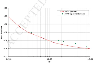
universal slope method and experimental data is presented in Figure 5, showing a good and slightly conservative

[image:10.595.107.487.447.705.2]

approximation.

Figure 5 Comparison between Modified Universal Slope Method and experimental results (Karakaş and Szusta, 2015). 0.00 0.01 0.01 0.02 0.02 0.03 0.03

1.E+02 1.E+03 1.E+04

S tr a in A m p li tu d e Nf

M

AN

US

CR

IP

T

AC

CE

PT

ED

10

Table 3 Temperature dependent tensile strength for 2024T3 aluminium alloy.

Su[MPa] 150°C 175°C 200°C

0.1 hr 550 436 460

1 hr 415 395 370

100 hrs 435 370 305

1000 hrs 400 330 260

In order to evaluate the creep rupture time the stress dependent reversed power-law is used:

* k

t

= ⋅

B

σ

− (12)

where B=1.93642E+017 and k=6.2252 are creep rupture material parameters estimated by fitting the experimental

creep rupture data available for the required temperature (175˚C for the creep-fatigue assessment). When the rupture

time is determined the time fraction rule is adopted to calculate the total creep damage. Once both the damages due to

fatigue

ω

fand creep ωcare calculated separately, a linear damage interaction

ω ω

f + c≤1is adopted to calculate the

total number of cycle to fail and the total damage as well.

4 Modified strain range partitioning

Strain range partitioning is a method for treating creep-fatigue interaction at elevated temperature where stress

mutiaxiality is involved. A full description of the strain range partitioning procedure is reported in (Manson and

Halford, 1976). Here, as suggested in (Manson and Halford, 1976), further studies have been undertaken in order to

understand the effect of anisotropy which arises in composite structures, non-proportional loading and high

temperature on the creep-fatigue interaction behaviour. Also, a modification of the method has been proposed aimed

at providing information on both the transition and steady-state behaviour. This procedure relies upon the comparison

between the ratchetting strain computed between two subsequent hysteresis loops and the ratchetting strain computed

within the hysteresis loop itself by using the strain range partitioning approach. A detailed description of the

procedure which is based on incremental FEA is reported in the following subsections. Comparison with the LMM

procedure is also reported in order to show the capability of the direct methods to provide feasible and computational

inexpensive solutions to assess the steady-state cyclic response.

4.1 Evaluation of the equivalent stress and strain

The first step is to compute the strain increments at each time instant within the cycle. We refer to 8 schematic

hysteresis loops that, as will be seen in the section 5, characterise the material response under the assigned loading

M

AN

US

CR

IP

T

AC

CE

PT

ED

11

[image:12.595.43.558.82.361.2]

Figure 6 Schematic steady state hysteresis loops for both SBS approach and LMM approach.

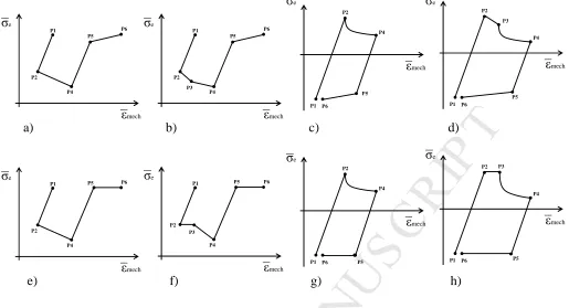
Figure 6a-b-c-d show the schematic steady state hysteresis loops related to the step-by-step (SBS) procedure while Figure 6e-f-g-h show the hysteresis loops related to the Linear Matching Method (LMM) procedure. The four loops

depicted in Figure 6a-b-e-f are referred to as total open loops (TOL) whereas the four loops depicted in Figure 6c-d-g-h are referred to as reverse open loops (ROL) if the points P1 and P6 are different while for P1=P6 they are referred

to as reverse closed loop (RCL). For both procedures the elastic strain increment in loading is computed between

points P1-P2, the plastic strain increment in loading between points P2-P3, the creep strain increment between points

P3-P4, the elastic strain increment in unloading between points P4-P5, and the plastic strain increment in unloading

between points P5-P6. It is noted that point P3 is present in the loops only when plastic strain in loading occurs.

Hence for the loops in Figure 6a-c-e-g the starting point of the creep phase is P2 and the creep strain increment is

computed between points P2-P4.

The main difference between the SBS procedure and the LMM procedure is in computing the load points P2 and P5

within the steady state hysteresis loop when plastic strain occurs in both loading and unloading. Indeed, as the yield

stress varies with the temperature (Table 1), the yield surface becomes smaller during the loading phase as the

temperature increases while during the unloading phase the yield stress increases as the temperature decreases. Thus,

the point P2 where the accumulation of plastic strain starts in loading for the loops in Figure 6b-d related to the SBS

procedure has an equivalent von Mises stress higher than the point P3 where the stress level is equal the yield stress at

the peak temperature within the thermal loading history. For the LMM procedure the point P2 depicted in Figure 6f-h

starts always at the same stress level as P3 which is equal to the yield stress at the peak temperature within the thermal

loading history. Same conclusion can be drawn for the point P5 where the accumulation of plastic strain starts in

P1 P2 P4 P5 P6 σe εmech P1 P2 P4 P5 P6 σe εmech P1 P2 P4 P5 P6 σe εmech P3 P1 P2 P4 P5 P6 σe εmech P3 P1 P2 P5 P6 σe εmech P4 P1 P2 P5 P6 σe εmech P4 P3 P1 P2 P5 P6 σe εmech P4 P1 P2 P5 P6 σe εmech P4 P3

a) b) c) d)

M

AN

US

CR

IP

T

AC

CE

PT

ED

12

unloading. As the yield surface increase during the unloading phase for the SBS procedure, point P5 has an equivalent

von Mises stress lower that the yield stress at room temperature (Figure 6b-d) while for the LMM procedure point P5

depicted in Figure 6f-h starts always from the same stress level as P6.

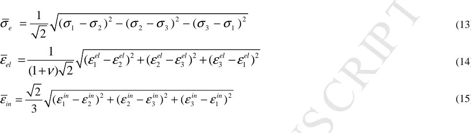
Let’s assume that the effect of the three principal components of stress and strain is characterized by single

parameters according to the equations:

2 2 2

1 2 2 3 3 1

1

(

)

(

)

(

)

2

e

σ

=

σ

−

σ

−

σ

−

σ

−

σ

−

σ

(13)

2 2 2

1 2 2 3 3 1

1

(

)

(

)

(

)

(1

) 2

el el el el el el

el

ε

ε

ε

ε

ε

ε

ε

ν

=

−

+

−

+

−

+

(14)

2 2 2

1 2 2 3 3 1

2

(

)

(

)

(

)

3

in in in in in in

in

ε

=

ε

−

ε

+

ε

−

ε

+

ε

−

ε

(15)

wherein

σ

_eis the equivalent stress at a generic cycle, time step, and time increment,

ε

_el is the equivalent elastic

strain and

ε

_inis the equivalent strain for the inelastic components where “in” can be “pl” (plastic), or “cr” (creep).

For both stress and strain the subscript “1”, “2” and “3” stands for maximum principal component, medium principal

[image:13.595.66.547.183.319.2]

component and minimum principal component, respectively.

Table 4. Strain increments at different load points of the stabilized hysteresis loop.

P1 P2 P3 P4 P5 P6

Elastic strain 1 P el

ε

2 P el

ε

∆

3 P el

ε

∆

4 P el

ε

∆

5 P el

ε

∆

6 P el

ε

∆

Plastic strain n/a n/a

3

P

pl

ε

∆

n/a n/a

6

P

pl

ε

∆

Creep strain n/a n/a n/a

4

P

cr

ε

∆

n/a n/a

Total inelastic

strain

ε

inP1

n/a n/a n/a n/a n/a

Upon defining the effective Young’s Modulus as

)

1

(

2

3

ν

+

=

E

E

_eff (EDF Energy, 2014) the six load points of the

stabilised hysteresis loops by means of the SBS procedure are computed using equation (13), (14), and (15) and the

strain increments for each load point within the loop are reported in Table 4. It is worth noting that the load point P1

is the last load point of the loop that precedes the stabilized loop. Hence

1

P

in

ε

is the accumulated inelastic strain from

the first cycle to the cycle that precedes the stabilized cycle.A similar approach is used by the LMM where all the

strain ranges and equivalent stresses are directly calculated for the stabilised hysteresis loop and stored in Abaqus

M

AN

US

CR

IP

T

AC

CE

PT

ED

13

4.2 Evaluation of the algebraic sign of the equivalent stress and strain

As seen in the section 4.1, all the equivalent values are evaluated in magnitude. For practical design situations for

which life prediction methods are intended to be used, often involve stresses in more than one direction. Thus, the

eventual usage of the strain-range partitioning method requires the entire stabilized stress-strain hysteresis loops to be

known. From the values of equivalent stress and strain at each point in the cycle, it then becomes possible to construct

an equivalent hysteresis loop wherein at each instant of time the stress is the equivalent stress and the strain is the

equivalent strain. However, before this can be done an algebraic sign to indicate tension or compression status must

be assigned to both magnitudes of equivalent stress and strain (Manson and Halford, 1976). The method proposed

comprises of two stages. The first stage is aimed at evaluating the algebraic sign of the equivalent stress and strain

within the first hysteresis loop. In particular, at each instant of time the equivalent stress and strain will be computed

according to (13), (14), and (15) but the algebraic sign of

σ

_e and

ε

_in will be the same as the one of the dominant

stress component i.e. the sign of the largest component between

σ

₁ and

σ

₃for the stress and the sign of the largest

component between 1

in

ε

and 3

in

ε

for the starin. Table 5 shows the sign of the first cycle related to the reference

transition hysteresis loops depicted in Figure 7. The circular, elliptical and square cross sections are referred to as

C11, C21, and S11 respectively within Table 5 where M0 stands for mechanical load

σ

p =0, M025 stands for

( 25)

0.25

p y

σ = ×σ , and M05 stands forσ_p =0.5×σ_y( 25). As previously mentioned, D1 stands for 1 hour of dwell time

and D100 stands for 100 hours of dwell period. Also, L, C, and U stand for end of loading phase, end of creep phase,

and end of unloading phase respectively.

Table 5. Sign of von Mises stresses at the first cycle for the reference transition hysteresis loops in Figure 7.

e

σ

σ

₁

σ

3 Sign

C11-M0-D1

L 322 56.0598 -313.566 -

C 254.933 46.2544 -249.238 -

U 92.2509 78.5282 -27.7436 +

C11-M025-D100

L 322 159.936 -183.87 -

C 179.248 128.372 -63.2164 +

U 312.495 300.479 -40.3999 +

C11-M05-D100

L 322 261.845 -78.3248 +

C 250.321 264.915 -22.5227 +

U 371 361.761 -16.3537 +

C21-M0-D100

L 322 232.372 -106.614 +

C 165.525 180.501 -2.45734 +

M

AN

US

CR

IP

T

AC

CE

PT

ED

14 C21-M025-D100

L 322 145.467 -209.131 -

C 149.572 88.3183 -70.7236 +

U 328.142 265.309 -74.3077 +

C21-M05-D100

L 322 191.087 -156.857 +

C 222.665 197.843 -51.489 +

U 371 293.351 -134.602 +

S11-M0-D100

L 322 365.054 -2.42783 +

C 188.02 278.731 61.8641 +

U 371 168.92 -232.541 -

With regards to the second stage, it is aimed at evaluating the sign of the hysteresis loop from the second cycle to the

stabilised cycle. Uppermost, we compute the ratchetting strain per cycle in three steps:

1. At the end of each load cycle, 6 components of the mechanical strain are obtained by subtracting

corresponding thermal strain components from total strain components. And then 6 components of the

ratchetting strain are calculated for each load cycle by the difference in corresponding components of

mechanical strain between the end and the beginning of each load cycle;

2. The equivalent ratchetting strain for each load cycle from the 2nd cycle to the stabilized cycle can then be

calculated by equation (15) since ratchetting strain is treated as inelastic strain;

3. Taking into account only the final steady state cycle, we compare the equivalent ratchetting stain rtch

ε

∆

with

the equivalent plastic strain increment in loading

3

P

pl

ε

∆

, the equivalent creep strain

4

P

cr

ε

∆

and the

equivalent plastic strain increment in unloading

6

P

pl

ε

∆

. Three scenarios can occur:

3 4 6

summ

rtch rtch pl_P cr_P pl_P

ε

ε

ε

ε

ε

∆

≅ ∆

= ∆

+ ∆

+ ∆

→

total open loop (TOL) (16)

3 4 6

diff

rtch rtch pl_P cr_P pl_P

ε

ε

ε

ε

ε

∆

≅ ∆

= ∆

+ ∆

− ∆

→

reverse open loop (ROL) (17)

3 4 6

0

rtch pl_P cr_P pl_P

ε

ε

ε

ε

∆

≅ → ∆

+ ∆

≅ ∆

→

reverse closed loop (RCL) (18)

M

AN

US

CR

IP

T

AC

CE

PT

ED

15

| |

% 100

summ

rtch rtch sum

rtch

err

ε

ε

ε

∆ − ∆

= ×

∆ (19)

| |

% 100

diff

rtch rtch diff

rtch

err

ε

ε

ε

∆ − ∆

= ×

∆ (20)

By computing the percentage error from equations (19) and (20), the stabilised hysteresis loops can be drawn and the

6 load points (5 if no plastic strain in loading occurs i.e. there is no point P3) are univocally determined in terms of

both magnitude and sign. Indeed a total open loop (TOL) is considered if % sum

err < %

diff

err instead a reverse open

loop (ROL) is considered if % sum

err > %

diff

err . It is worth pointing out that a TOL in this paper is a hysteresis loop

where the von Mises stress at each load point is always positive as shown in Figure 6a-b-e-f. Instead, a ROL can

have either the stresses of both the loading and creep phase positive and the stresses of the unloading phase negative

as shown in Figure 6c-d-g-h or vice versa.

5 Application of the concepts to MMCs and discussions

5.1 Transition behaviour

As discussed in section 4, we proposed a variation of the strain range partitioning in order to evaluate both the

[image:16.595.42.552.444.695.2]

transition behaviour and the steady state behaviour of long fibre MMCs.

M

AN

US

CR

IP

T

AC

CE

PT

ED

16

Further explanations on the latter behaviour will be provided in subsection 5.2. Here, a physical explanation of the

transition behaviour that justifies the method adopted is discussed. Detailed results are only presented for the steady

state behaviour whereas the transition behaviour is discussed in a schematic way. This methodology can be applied to

different integration points within the structures in order to find the most critical location to assess. Here, for all the

geometries considered, the integration point chosen is the one with the highest creep damage.

Figure 7 shows the schematic transition behaviour for the 3 cross-sections studied for different mechanical loads and

dwell times. Contours of the creep strain increment at the stabilised cycle

4

P

cr

ε

∆

show the area where the highest

creep damage occurs. As discussed in section 3, the load points investigated experience shakedown for both the

circular cross-section and the elliptical cross-section if no creep dwell is introduced. Instead reverse plasticity

behaviour is expected for the square cross-section. By introducing a creep dwell within the cyclic thermal loading at

the tensile peak, different scenarios arise as reported in (Barbera et al., 2016b) for metallic structures at elevated

temperature. Here a new mechanism is seen when the off-axis constant mechanical load in Figure 4-b, is applied.

Indeed, for small creep dwell e.g. D1 and no mechanical load M0, the composite with the circular cross-section

remains in shakedown while for D100 it experiences a reverse closed loop (RCL). These two material responses have

already been discussed in (Barbera et al., 2016b). By increasing the mechanical load e.g. M025, there is a sign

variation that leads the structures to experience creep-ratchetting with a total open loop (TOL). This is because the

thermal load and the mechanical load act in the opposite direction so that the more the thermal stress relaxes the more

the mechanical load becomes predominant. For the highest mechanical load applied, M05, the equivalent stress is

positive in loading because the mechanical load is predominant from the first cycle. With regards to the elliptical

cross-section, for M0 and all the dwell times, a steady state reverse closed loop response is seen after a transition

phase where a sequence of reverse loops show creep-ratchetting. Compared to the circular cross-section, the reverse

closed loops of the elliptical cross-section have the stresses of the loading and creep phases positive from the first

cycle (Table 5) to the stabilised one. This is mainly due to the positive value of the stress component along the y

direction as it affects the magnitude of the maximum principal component

σ

₁such that it becomes predominant

during the loading compared to the minimum principal component

σ

₃. Instead for the circular cross-section the

magnitude of the minimum principal component

σ

₃is affected by the stress component along the fibre direction z.

Therefore the magnitude of

σ

₃ is higher than

σ

₁ during loading and lower than

σ

₁during unloading. Regarding the

square cross-section the creep dwell leads the structure to experience negative reverse ratchetting after a transition

phase where the structure experiences positive ratchetting with a reverse open loop. This because the stress relaxation

enhances the plastic strain in unloading which after a certain number of cycles is not more compensated by the

M

AN

US

CR

IP

T

AC

CE

PT

ED

17

5.2 Steady-state behaviour

The steady-state cyclic stress-strain hysteresis loops for the three geometries studied are presented. Full inelastic

step-by-step simulations have been used to verify the LMM results. Modified strain range partitioning, described in section

4, has been used. All the strain increments, ratchetting strains per cycles, and percentage errors are reported in tabular

form in order to facilitate the understanding of the method adopted.

Table 6. Circular cross-section stress and strain ranges for the stabilised hysteresis loops for D100.

3 P e

σσσσ

4 P e

σσσσ

6 P e

σσσσ

3 P pl

εεεε

∆∆∆∆

4 P cr

εεεε

∆∆∆∆

6 P pl

εεεε

∆∆∆∆

rtch

εεεε

∆∆∆∆

LMM 52.4787 50.858 371 0.00E+00 2.60E-05 2.30E-05 3.00E-6

M0

SBS 46.089 45.074 371 0.00E+00 1.71E-05 1.79E-05 8.00E-7

LMM 138.516 134.053 371 0.00E+00 6.38E-04 1.78E-04 6.84E-04

M025

SBS 138.694 133.922 371 0.00E+00 6.32E-04 1.82E-04 6.73E-04

LMM 291.982 252.392 371 0.00E+00 6.17E-03 1.83E-03 7.35E-03

M05

SBS 296.096 249.94 371 0.00E+00 5.88E-03 2.18E-03 7.14E-03

Table 7. Circular cross-section’s percentage error for the stabilised hysteresis loops for D100.

rtch

εεεε

∆∆∆∆

summ rtch

εεεε

∆∆∆∆

diff rtch

εεεε

∆∆∆∆

% sum err % diff

err M Loop

LMM 3.00E-6 4.90E-05 3.00E-06 1533.33% 0.00%

M0 RCL

SBS 8.00E-7 3.50E-05 8.00E-07 4275.00% 0.00% RCL

LMM 6.84E-04 8.16E-04 4.60E-04 19.30% 32.75%

M025 TOL

SBS 6.73E-04 8.14E-04 4.50E-04 20.95% 33.14% TOL

LMM 7.35E-03 8.00E-03 4.34E-03 6.24% 42.36%

M05 TOL

SBS 7.14E-03 8.06E-03 3.70E-03 12.89% 48.18% TOL

Table 6 reports for the circular cross-section the stress and strain ranges computed by the LMM and SBS for the three

different load points A1, A2, and A3 in Figure 4-a and for a dwell time of 100 hours. Comparing the results of both

approaches, it can be seen that the LMM overestimates the plastic strain range in unloading

6

P

pl

ε

∆

and the creep

strain range

4

P

cr

ε

∆

for M0. Instead for M025 and M05 the highest percentage error is lower than 16%. The

correlation between the ratchetting percentage errors and the type of hysteresis loop for the circular cross-section is

shown in Table 7. All the data are computing according to the equations (16), (17), (18), (19) and (20). What can be

clearly seen in Table 7 is that for M0, a closed reverse loop is considered as

0

rtch

ε

∆

≅

. When the mechanical load

increases e.g. M025 or M05, a total open loop is seen as % diff

err is higher than % sum

M

AN

US

CR

IP

T

AC

CE

PT

ED

[image:19.595.43.561.70.418.2]

18

Figure 8 Steady-state hysteresis loops for the circular cross-section for three dwell times (1hr, 10hrs, 100hrs) and three mechanical load (σσσσ_p====0,σσσσp ====0.25××××σσσσ(y25),σσσσp ====0.5××××σσσσ(y25)).

Figure 8 shows all the stabilised hysteresis loops for the circular cross-section for all the load scenarios investigated.

As we have seen in Figure 7 with regard to the circular cross-section, when the mechanical load is equal zero, there is

no sign variation during the stress relaxation and the structure exhibits either shakedown for small dwell times i.e. D1

or reverse plasticity for longer dwell time i.e. D10 and D100. When the off-axis mechanical load is applied the

stabilised loop is a total open and creep-ratchetting occurs.

Table 8. Elliptical cross-section stress and strain ranges for the stabilised hysteresis loops for D100.

3

P

e

σσσσ

4

P

e

σσσσ

6

P

e

σσσσ

3

P

pl

εεεε

∆∆∆∆

4

P

cr

εεεε

∆∆∆∆

6

P

pl

εεεε

∆∆∆∆

rtch

εεεε

∆∆∆∆

LMM 226.949 142.733 371 0.00E+00 1.54E-03 1.56E-03 2.00E-5

M0

SBS 228.033 141.01 371 0.00E+00 1.56E-03 1.55E-03 1.00E-5

LMM 243.826 176.375 371 0.00E+00 2.50E-03 3.01E-03 4.66E-03

M025

SBS 247.21 170.436 371 0.00E+00 2.32E-03 3.46E-03 4.61E-03

LMM 322.127 267.454 371 1.14E-03 7.95E-03 4.76E-02 5.54E-02

M05

[image:19.595.17.578.587.710.2]

M

AN

US

CR

IP

T

AC

CE

PT

ED

[image:20.595.38.559.82.204.2]

19

Table 9. Elliptical cross-section’s percentage error for the stabilised hysteresis loops for D100.

rtch

εεεε

∆∆∆∆

summ

rtch

εεεε

∆∆∆∆

diff

rtch

εεεε

∆∆∆∆

%

sum

err %

diff

err M Loop

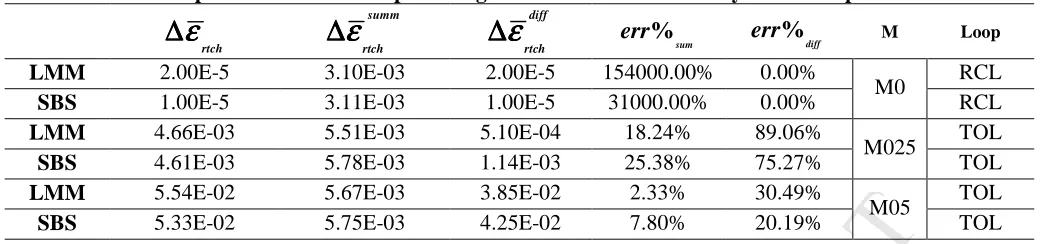
LMM 2.00E-5 3.10E-03 2.00E-5 154000.00% 0.00%

M0 RCL

SBS 1.00E-5 3.11E-03 1.00E-5 31000.00% 0.00% RCL

LMM 4.66E-03 5.51E-03 5.10E-04 18.24% 89.06%

M025 TOL

SBS 4.61E-03 5.78E-03 1.14E-03 25.38% 75.27% TOL

LMM 5.54E-02 5.67E-03 3.85E-02 2.33% 30.49%

M05 TOL

SBS 5.33E-02 5.75E-03 4.25E-02 7.80% 20.19% TOL

Table 8 compares the stress and strain ranges between LMM and SBS with regards to the elliptical cross-section at

D100. Here the LMM overestimates the creep strain range when the mechanical load is M05. For all the other ranges

the percentage error is lower than 13%. Table 9, provides the intercorrelations between the percentage errors and the

type of hysteresis loop for the elliptical cross-section. As previously discussed for the circular cross-section, when the

mechanical load is equal to zero, a closed reverse loop is considered. Instead, creep-ratchetting is seen in the form of

[image:20.595.42.563.318.679.2]

total open loop for M025 and M05.

M

AN

US

CR

IP

T

AC

CE

PT

ED

20

With regard to the stabilised hysteresis loops for the elliptical cross-section shown in Figure 9 for all the dwell times

investigated the structure’s response is in agreement with the results provided in Table 9. For M05, the main

difference between the elliptical cross-section and the circular cross-section is that the open loops for the former

accumulate plastic strain in loading and unloading. This leads the structure to experience a higher ratchetting strain

[image:21.595.16.578.189.314.2]

per cycle compared to the scenario with M025.

Table 10. Square cross-section stress and strain ranges for the stabilised hysteresis loops for D100.

3 P e

σσσσ

4 P e

σσσσ

6 P e

σσσσ

3 P pl

εεεε

∆∆∆∆

4 P cr

εεεε

∆∆∆∆

6 P pl

εεεε

∆∆∆∆

rtch

εεεε

∆∆∆∆

LMM 322 185.855 371 2.51E-03 4.17E-03 6.91E-03 2.71E-04

M0

SBS 322 183.691 371 2.51E-03 4.06E-03 6.83E-03 3.00E-04

LMM 322 185.443 371 2.52E-03 4.06E-03 7.15E-03 5.47E-04

M025

SBS 322 184.072 371 2.47E-03 4.06E-03 7.09E-03 5.02E-04

LMM 322 198.515 371 2.97E-03 4.69E-03 1.00E-02 2.69E-03

M05

SBS 322 210.653 371 3.01E-03 4.66E-03 1.01E-02 2.65E-03

Table 11. Square cross-section’s percentage error for the stabilised hysteresis loops for D100.

rtch

εεεε

∆∆∆∆

summ rtch

εεεε

∆∆∆∆

diff rtch

εεεε

∆∆∆∆

% sum err % diff

err M Loop

LMM 2.71E-04 1.36E-02 2.30E-04 4914.76% 15.13%

M0 ROL

SBS 3.00E-04 1.34E-02 2.60E-04 4366.67% 13.33% ROL

LMM 5.47E-04 1.37E-02 5.70E-04 2410.05% 4.20%

M025 ROL

SBS 5.02E-04 1.36E-02 5.60E-04 2613.15% 11.55% ROL

LMM 2.69E-03 1.77E-02 2.34E-04 556.51% 13.01%

M05 ROL

SBS 2.65E-03 1.78E-02 2.43E-04 570.57% 8.30% ROL

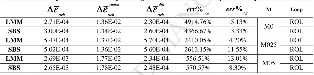
Table 10 reports the stress and strain ranges at D100 for the square cross-section for the three load scenarios

considered. Here the comparison between LMM and SBS shows a percentage error for all the strain ranges lower than

3%. Table 11 shows the same information as the previous cross-sections investigated reported in Table 7 and Table 9. Here reverse open loops are considered for all the load scenarios as %

diff

err is always lower than % sum

[image:21.595.44.556.335.458.2]

M

AN

US

CR

IP

T

AC

CE

PT

ED

[image:22.595.39.573.70.418.2]

21

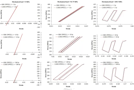
Figure 10 Steady-state hysteresis loops for the square cross-section for three dwell times (1hr, 10hrs, 100hrs) and three mechanical load (σσσσ_p====0,σσσσ_p ====0.25××××σσσσ(_y25),σσσσ_p ====0.5××××σσσσ(_y25)).

Figure 10 shows the stabilised hysteresis loops for the square cross-section for all the mechanical loads and dwell

times. As we have seen in Figure 7 the square cross-section shows a reverse ratchetting at the stabilised loop after a

certain number of cycles during the transition phase. This is because during the transition phase the sum of the plastic

strain in loading

∆

ε

Lpland the creep strain

∆

ε

cr is higher than the plastic strain in unloading U

pl

ε

∆

.Therefore the

loop moves rightward until

∆

ε

Upl is lower than the aforementioned sum. When U

pl

ε

∆

becomes dominant the

steady-state cycle moves leftward. From Figure 10 it is clear that the higher the dwell time the sooner the transition

from the rightward ratchetting to a leftward ratchetting is reached.

6 Creep fatigue and creep ratchetting assessment

The assessment of the microstructures has been done by considering the effect of the steady-state on the crack

initiation process. As depicted in Figure 7, by changing the applied load and fibre geometry the steady-state response

can change remarkably. The scope of this section is to understand and provide more information on how these

responses could trigger crack initiation within the metal matrix. It worth noting that the matrix and the fibre are

M

AN

US

CR

IP

T

AC

CE

PT

ED

22

6.1 Cyclic thermal load without transverse mechanical load

When no mechanical load is applied, only the thermal stress caused by the coefficient of thermal expansion mismatch

is present. For this condition, the best geometry is the circular one, as the response is strict shakedown for small dwell

times i.e. D1 and closed loop for longer dwell times i.e. D10 and D100 as shown in Figure 8. For the ellipse and the

square section, a closed reverse loop response has been observed for all the dwell times investigated as shown in

Figure 9 and Figure 10. In both cases the creep-fatigue interaction lead to the initiation of a crack within the matrix

and it is driven by the creep damage. In both the geometries, the thermal stresses are subjected to a large stress

relaxation as shown in Figure 11a. The stress relaxation is responsible for the creep damage accumulated during each

creep dwell. The trend of the stress relaxation is very similar but the stress at the start of the creep dwell is much

higher for the square fibre. In turn, as depicted in Figure 11b, the creep strain accumulated during the increasing

creep dwell is larger for the square geometry. This is caused by the higher stress occurring during the creep dwell.

The large creep strain accumulation and stress relaxation exhibited by the square fibre is the main cause of reversed

creep ratchetting shown in Figure 7. However, this ratchet strain per cycle is small and compressive preventing any

fracture due to excessive deformation.

Figure 11 a) Stress relaxation and b) creep strain accumulation during increasing creep dwell.

In terms of overall creep fatigue life, which in both cases is dominated by the creep damage, the ellipse performs

generally better than the square fibre as reported in Figure 12. This is due to the higher stress at the start of the creep

dwell of the square fibre, which is 322 MPa against the 226 MPa of the elliptic fibre. For increasing dwell time the

endurances predicted for both the geometries reduce significantly. The decrease in creep-fatigue life is nearly linear

for the geometries investigated suggesting that both are affected in a similar way by the creep dwell length.

100 150 200 250 300 350

0 20 40 60 80 100

S

tr

es

s

[M

P

a

]

Dwell time [hours]

Ellispe Square

a)

0.0E+00 5.0E-04 1.0E-03 1.5E-03 2.0E-03 2.5E-03 3.0E-03 3.5E-03 4.0E-03 4.5E-03

0 20 40 60 80 100

C

re

ep

s

tr

a

in

Dwell time [hours]

Ellispe Square

[image:23.595.98.505.342.508.2]

M

AN

US

CR

IP

T

AC

CE

PT

ED

23

Figure 12 Creep-fatigue endurances for the ellipse and circle fibres without mechanical load.

The failure mechanism associated to the cyclic thermal load for a creep dwell of 100 hours is depicted in Figure 13

for both cases. The ellipse has expected life of 36 cycles and the area where the damage initiate is shown in Figure 13a. The blue area is relatively large and spread on both fibre sides along the vertical axis. Commonly creep-fatigue

failure mechanism is considered a localized mechanism associated to the initiation of a crack, as it is for the square

(Figure 13b). However, for the elliptical cross section a remarkable volume of material is expected to fail. This can

be explained by considering the effect of the fibre geometry, which enhances the geometrical constraint between each

fibre. Conversely, for the square the failure mechanism is localized at the inner edge of the square fibre, where the

stresses are at the highest point. This causes a significant reduction in creep-fatigue life, which for the case considered

[image:24.595.195.499.75.249.2]

is only 3 cycles.

Figure 13 Creep-fatigue life of the a) ellipse and b) square fibre subjected to a cyclic thermal load and a creep dwell of 100 hours.

6.2 Cyclic thermal load with a transverse mechanical load

When a mechanical load is applied, all the geometries analysed tend to exhibit creep ratchetting, which competes with

creep-fatigue crack initiation. The increase of dwell time enhances the creep and fatigue damage in all the geometries.

Also, creep-ratchetting is affected by the dwell time considered and the magnitude of inelastic strain accumulated at

each cycle also increases with the mechanical load. When a constant transverse mechanical of 92.75 MPa is applied,

creep-fatigue interaction and creep-ratchetting compete. For circular and elliptical cross-section, Figure 14a-b,

creep-fatigue interaction is dominant up to a threshold. This threshold is dependent on the cross-section and is around 30

1 10 100 1000

1 10 100

C

y

cl

es

t

o

f

a

il

u

re

Dwell time [hr]