City, University of London Institutional Repository
Citation:
Papoutsakis, A., Rybdylova, O. D., Zaripov, T. S., Danaila, L., Osiptsov, A. N.
and Sazhin, S. S. (2018). Modelling of the evolution of a droplet cloud in a turbulent flow.
International Journal of Multiphase Flow, 104, pp. 233-257. doi:
10.1016/j.ijmultiphaseflow.2018.02.014
This is the accepted version of the paper.
This version of the publication may differ from the final published
version.
Permanent repository link:
http://openaccess.city.ac.uk/20661/
Link to published version:
http://dx.doi.org/10.1016/j.ijmultiphaseflow.2018.02.014
Copyright and reuse: City Research Online aims to make research
outputs of City, University of London available to a wider audience.
Copyright and Moral Rights remain with the author(s) and/or copyright
holders. URLs from City Research Online may be freely distributed and
linked to.
City Research Online: http://openaccess.city.ac.uk/ [email protected]
Modelling of the evolution of a droplet cloud in a turbulent flow
Andreas Papoutsakisa,∗, Oyuna D. Rybdylovaa, Timur S. Zaripova,b, Luminita Danailac, Alexander N. Osiptsovd,
Sergei S. Sazhina
aSir Harry Ricardo Laboratories, Advanced Engineering Centre, School of Computing, Engineering and Mathematics, University of Brighton,
Brighton, BN2 4GJ, UK.
bHigh Performance Distributed Computing Laboratory, Kazan Federal University, 420097, Kazan, Russia cCORIA, UMR 6614, Universit´e de Rouen, Avenue de l’Universit´e, BP 12, 76801 Saint Etienne du Rouvray, France
dInstitute of Mechanics, Lomonosov Moscow State University, Michurinskii 1, 119899, Moscow, Russia
Abstract
The effects of droplet inertia and turbulent mixing on the droplet number density distribution in a turbulent flow field are studied. A formulation of the turbulent convective diffusion equation for the droplet number density, based on the modified Fully Lagrangian Approach, is proposed. The Fully Lagrangian Approach for the dispersed phase is extended to account for the Hessian of transformation from Eulerian to Lagrangian variables. Droplets with moder-ate inertia are assumed to be transported and dispersed by large scale structures of a filtered field in the Large Eddy Simulation (LES) framework. Turbulent fluctuations, not visible in the filtered solution for the droplet velocity field, induce an additional diffusion mass flux and hence additional dispersion of the droplets. The Lagrangian formulation of the transport equation for the droplet number density and the modified Fully Lagrangian Approach (FLA) make it possible to resolve the flow regions with intersecting droplet trajectories in the filtered flow field. Thus, we can cope successfully with the problems of multivalued filtered droplet velocity regions and caustic formation. The spatial derivatives for the droplet number density are calculated by projecting the FLA solution on the Eulerian mesh, result-ing in a hybrid Lagrangian-Eulerian approach to the problem. The main approximations for the method are supported by the calculation of droplet mixing in an unsteady one-dimensional flow field formed by large-scale oscillations with an imposed small-scale modulation. The results of the calculations for droplet mixing in decaying homogeneous and isotropic turbulence are validated by the results of Direct Numerical Simulations (DNS) for several values of the Stokes number.
Keywords: Fully Lagrangian Approach, turbulent diffusion, droplet mixing, second order structure, caustics
1. Introduction
The analysis of droplet dynamics and their spatial distribution in turbulent flows is important for various engineer-ing applications, rangengineer-ing from fuel injection in internal combustion engines to droplet dispersion in environmental flows (e.g. Sazhin (76)). Inertial droplets suspended in turbulent flow fields undulate under the influence of flow fluctuations along their trajectories. The droplet velocities are controlled by both the history of the droplet motion and the spatially correlated structures of the turbulent flow field. A variety of characteristic responses of the discrete phase to the turbulent fluctuations of the carrier phase have been identified. These responses include the macro-scopic scale turbulent mixing (Fung et al. (27)), de-mixing or un-mixing of particles (Fessler et al. (22), Reeks (70)), Random Uncorrelated Motion (RUM) (Meneguz and Reeks (51)) and increasing settling velocity (Wang and Maxey (89), Maxey (49)). In large-scale engineering and environmental applications, the behaviour of sufficiently low-inertia droplets/particles, characterised by small values of the Stokes number (the ratio of the droplet velocity relaxation time to the macro time scale) in turbulent flows, has been successfully described by the convective diffusion equation with different models for the turbulent diffusion coefficient (Fuchs (25), Berlyand (3)).
∗
Two approaches are commonly used for the analysis of turbulent droplet/particle laden flows: Eulerian-Eulerian and Eulerian-Lagrangian (see Marchioli (46), Simonin et al. (81)). In the Eulerian-Eulerian approach several versions of the two-fluidk−εmodel have been used (Pakhomov and Terekhov (58)). The Eulerian-Eulerian approach gives satisfactory results for describing large-scale structures and some integral parameters of turbulent gas-particle flows in channels, jets, and boundary layers. In this approach, uniqueness of all parameters of the particulate continuum is assumed. However, the mesoscale flow regions with possible formation of local droplet accumulation zones are associated with intersecting droplet trajectories and caustics in the dispersed-phase velocity field. The appearance of local regions of intersecting droplet trajectories with singularities in the droplet number density on the edges of these regions (caustics), and the types of these singularities in non-uniform and unsteady flows with inertial droplets, were described by Osiptsov (56). Further investigations can also be found in Falkovich et al. (19) and Wilkinson et al. (90). Classes of two-particle models that allow for singularities in the phase space and intersecting trajectories (see Zaichik and Alipchenkov (93, 94), Chun et al. (14), Gustavsson and Mehlig (31), Pan and Padoan (59)), are presented in (6, 5). Also, Eulerian models for the particulate continuum inferred from the kinetic equations for particles or from the equations for the probability density functions (PDF) of particles are presented by Zaichik et al. (95) and by Shrimpton et al. (80). In engineering publications on turbulent gas-droplet flows, the carrier flow field has been described on the filtered scale, with the system of droplets described in the framework of the continuum approximation (e.g. Volkov and Emelianov (87)).
In many engineering applications (e.g. fuel spray injection and mixing, two-phase flows in combustion chambers), it is important to have information about the structure of local particle/droplet accumulation zones to estimate the rates of possible droplet collisions and the effect of droplet accumulation on heating and evaporation of droplets and combustion of fuel vapour/air mixtures (76). This information can be inferred only from Lagrangian tracking of the dispersed phase. In the standard Eulerian-Lagrangian approach for gas-particle/droplet flow modelling (e.g. Crowe et al. (16); Sazhin (76)), the carrier-phase flow parameters are calculated on a fixed Eulerian mesh and the particles/droplets are tracked along chosen Lagrangian trajectories. Direct modelling of individual droplet trajectories in the carrier phase leads to satisfactory results for the droplet velocity field (e.g. Sazhina et al. (77)). However, the correct calculation of the droplet number density field presents serious difficulties. This was instructively demonstrated by Healy and Young (35), who showed that to reach a satisfactory accuracy in the calculation of the droplet number density in a laminar flow it is necessary to have about 103Lagrangian droplet trajectories per Eulerian cell.
An approach that incorporates the solution of the droplet number conservation equation in Lagrangian form is the Fully Lagrangian Approach (FLA). In the paper by Healy and Young (35) it was demonstrated for laminar flows that the number density of non-colliding particles along a chosen particle trajectory, and the trajectory itself, can be much more efficiently calculated based on the Fully Lagrangian Approach (FLA) proposed by Osiptsov (56) (see also (Osiptsov (57))). FLA is based on the Lagrangian form of the continuity equation for the particulate phase, treated as a continuum, and the additional equations for the components of the Jacobi matrix of transformation from the Eulerian to the Lagrangian coordinates. This is essentially a method of characteristics for the solution of the continuity equation on the Lagrangian trajectories. This approach can deal with such complex cases as the regions of intersecting droplet trajectories and caustics. In (39), the efficiency of the FLA for the calculation of the droplet number density and its modelling capability in identifying the spatial structure of caustics was demonstrated.
The introduction of the FLA into the study of turbulent flows (see Picciotto et al. (65)) resulted in the identification and analysis of spatial structures of the dispersed phase distribution using the moments of concentration. The analysis by Meneguz and Reeks (51) showed that the distribution of the particle concentration in the long term is log normal. This is consistent with the analysis by Monchaux et al. (53) where, using Vorono¨ı tessellation, the authors observed the same log normal distribution. Also, FLA studies on DNS of homogeneous and isotropic turbulence led to identification of the mechanisms involved in the segregation process (51, 70). The introduction of the FLA in the study of turbulent flows resulted in the quantification of the singularities related to trajectory intersections and the establishment of a relation between the frequency of their occurrence and the Stokes number.
Lebedeva et al. (43) proposed a method based on a combination of the Lagrangian viscous-vortex method for the carrier phase and the Fully Lagrangian Approach for the dispersed phase. This is the fully mesh-less approach which makes it possible to avoid a cumbersome procedure of remeshing the dispersed phase parameters from the Eulerian to Lagrangian grids, which is typical for standard Eulerian-Lagrangian approaches.
In some publications (e.g. Picciotto et al. (65), Meneguz and Reeks (51), Reeks (70)), the Fully Lagrangian Approach for the dispersed phase was used alongside the DNS calculations of the carrier phase flow fields in a turbulent channel flow and in forced homogeneous turbulence simulations. These authors identified the formation of multiple singularities in the particle concentration fields.
Note that the carrier-phase velocity fluctuations lead to increased dispersion of suspended particles/droplets (here-after referred to as droplets) which can be identified as turbulent mixing (see Reeks (68)). Analogies between the mixing of droplets in turbulent flows and Brownian diffusion have been drawn by Xia et al. (92) and Fung et al. (27). This allows one to assume that the interaction between discrete phase and small scale turbulent fluctuations can be regarded as a Fickian diffusion process. Also, it has been observed that coherent turbulent structures of the carrier phase induce segregation of droplets at least at the level of the integral length scale of the flow field (Fessler et al. (22)), and the formation of patterns as described by Wood et al. (91), and by Soldati and Marchioli (82).
Droplet dispersion in turbulent droplet laden flows has been found to be far more sophisticated than the scalar mixing of a contaminant in a turbulent flow field (see Reeks (68), Fessler et al. (22)). It was shown that the turbulence of the carrier phase is responsible not only for droplet turbulent mixing (Fickian diffusion) (see Phythian (64)), but also for the un-mixing of droplets to form coherent structures controlled by the integral length scale of the turbulent flow field (see Fessler et al. (22), Ijzermans et al. (38)) and their accumulation in caustic formations. Thus, mixing and un-mixing processes in this case can co-exist (Xia et al. (92)).
In addition to mixing, dispersed flows exhibit a wide range of responses to the fluctuation of the carrier phase flow field. With increasing droplet inertia (Stokes number), the effects of memory on the droplet motion become more pronounced. Direct numerical simulation of the behaviour of inertial droplets in forced isotropic turbulence shows that, as a rule, the distribution of inertial droplets in a turbulent velocity field is markedly non-uniform. Maxey (49) identified the segregation of droplets by a ‘preferential concentration’ clustering mechanism (34), in the regions of high strain rate for small Stokes numbers. This clustering is correlated with the underlying instantaneous carrier flow velocity field. Squires and Eaton (84) observed the formation of narrow local droplet accumulation regions in the zones of low vorticity and high strain rate. In a series of publications by Vassilicoset al. (e.g. Chen et al. (13)), the particle accumulation zones are associated with the zero-acceleration points.
High inertia droplets sample the carrier phase velocity field as a white noise (Gustavsson and Mehlig (32)), in an ergodic fashion, forming clusters due to the ‘multiplicative amplification’ mechanism (90, 31, 32). Recently, this multiplicative process of amplification and dilatation was identified by Meneguz and Reeks (51) as the deformation of the Lagrangian volume of the dispersed phase (Osiptsov (56)) transported along a particle trajectory. This volume may vanish at isolated singular points, giving rise to instantaneous singularities in the particle concentration field.
In the same work (51), in addition to mixing and un-mixing (clustering), a third type of characteristic response of the dispersed phase in turbulent flows, applicable to all Stokes numbers, has been suggested. This is known as Random Uncorrelated Motion (RUM). The occurrence of RUM was linked with the occurrence of singularities due to trajectory intersections related to the trajectory history. Particle motion, as the overlapping of a mesoscopic smoothly varying component and RUM, was identified in (23, 48, 97). RUM results in a multivalued velocity field of the dispersed phase due to the folding of the dispersed continuum, playing a significant role in collision processes.
The modelling challenge introduced by the presence of turbulent fluctuations in engineering flows is related to the wide range of turbulent length scales. Any flow field can be characterised by certain macroscopic scales. The turbulent cascade of the large macroscopic eddies to the smallest scales, controlled by viscosity, leads to a flow structure which is too detailed to be accurately represented. For many practical applications, the DNS of the carrier flow field is not feasible due to the complexity of the flow geometry and high Reynolds numbers. For real life flows it becomes computationally prohibitive to obtain a solution at the required resolution. Hence, filtering or averaging operators are imposed on the governing equations. The aim is to reduce the complexity of the problem by avoiding the full resolution of the whole range of turbulent scales.
trajectories and the formation of local zones of multivalued droplet parameters and caustics.
In the present study, we suggest a new approach combining LES calculations of the carrier phase flow field and the Fully Lagrangian Approach (FLA) for the dispersed phase. This is essentially a generalisation of the FLA for the analysis of droplets in filtered turbulent flows. Our approach is based on the following assumptions:
(i) in the averaged (filtered) flow of the carrier phase, droplets can be treated as a pressureless continuum; (ii) in the droplet continuity equation written in the Lagrangian form, subgrid random fluctuations of the carrier phase velocity result in an additional mass flux, which can be described by a Fickian law with a scalar droplet turbulent diffusion coefficient;
(iii) in calculating the droplet number density along a chosen trajectory, spatial derivatives of the number density are found by projecting the FLA solution on the Eulerian mesh; this results in a hybrid Lagrangian-Eulerian approach to the problem of calculation of the droplet concentration.
Basic principles of the FLA are summarised in Section 2. The generalisation of this approach to the analysis of the evolution of a droplet cloud in a turbulent flow is presented in Section 3. The validity of some of the assumptions, on which the model described is based, is also illustrated in Section 3, using the analysis of a simple one-dimensional flow. In Section 4 the second order extension of the FLA to describe the spatial structure of the number density field is presented and demonstrated. In Section 5, numerical experiments to determine the spatial structure of a turbulent flow field in a box with homogeneous decaying turbulence are described. In the same Section the model predictions are compared with the DNS predictions. In Section 6, the motivation behind the modelling choices made for the derivation of the modified FLA is discussed. The main results of the paper are summarised in Section 7.
2. The Fully Lagrangian Approach
In this section we present the framework of the Fully Lagrangian Approach (FLA) used for the modelling of a particulate medium dispersed in a fully resolved (laminar) carrier phase flow field. We set out the governing equations for the conservation of mass and momentum used in the FLA.
The droplets are assumed to be identical spheres of massmdand radiusσ. Assuming the point particle
approxima-tion, inter-particle collisions can be ignored. Thus, ignoring the Brownian motion of the droplets, the velocity of the dispersed phase at each point in the dispersed-phase continuum is singularly defined. This implies that the probability density function for the droplet distribution over velocities is the Dirac delta-function, and the velocity of a sampling droplet coincides with the velocity of the dispersed-phase continuumVd. The dispersed phase continuum is defined
in a space with possible folds; thus,Vd can be multivalued. Hence, the trajectory of a droplet, coinciding with the
trajectory of an elementary volume of the droplet continuum, is described by the following kinematic equation:
dxd
dt =Vd. (1)
Iff is the force exerted on the droplet by the fluid, the velocity of the droplet continuum can be found from the momentum equation for a droplet:
md
dVd
dt =f. (2)
Equation (2) follows from the momentum equation for a pressureless continuum, as described in (45).
Note that the very dilute particulate continuum, introduced in FLA, is in some sense ‘artificial’. This particulate continuum can penetrate itself since the droplet trajectories can intersect, forming ‘creases’ and ‘folds’. This means that the continual variableVd(x,t) can be multivalued, at least in some regions where droplet trajectories intersect.
This makes it difficult to describe this dispersed continuum using the Eulerian approach since the momentum and continuity equations in the Eulerian variables assume that all parameters are single-valued. Alternatively, one could use the Lagrangian approach to describe the particulate medium. Equations (1) and (2) can be regarded as Lagrangian equations if the variables (xd) andVdare considered as the functions of Lagrangian coordinatesxd
0and timet. In what
Introducing the droplet number densityndas the mean number of droplets per unit volume, we can formulate the continuity equation of the droplet medium in the integral form:
d dt
Z
VL(t)
nddxd=0, (3)
where,VL(t) is an arbitrary Lagrangian volume of the droplet continuum, each point of which travels at the droplet
velocityVd(xd,t), wherexdis the radius vector of the point in a Cartesian coordinate system.
Introducing Lagrangian variablesxd
0andt(x
d
0 =(x
d
0,y
d
0,z
d
0) are the coordinates of the radius vector of the point at
the initial instant of timet=0), we can rewrite this equation as:
d dt
Z
V0
nd(x0,t)det
Ji j(x0,t)
dx0=0, (4)
where, det(J(x0,t)) is the determinant of the Jacobi matrix for the transformation from the Eulerian to the Lagrangian
coordinates, defined as:
Ji j = ∂x
d i ∂xd
0,j
, (5)
xd
i is theith component of the radius vector of the point in the droplet cloud at time instantt, and x d
0,j is the jth
coordinate of this point at the initial time instantt =0. The introduction of the Jacobian of the transformation from the Lagrangian to the Eulerian coordinates implies that the transformationx(x0,t) is continuous and differentiable.
In (4), the integration is performed over the initial volumeV0=VL(t=0). SinceV0does not depend on time, the
order of time differentiation and spatial integration can change. Since this equation is valid for an arbitrary volume
V0, the continuity equation for the droplets can be written in the differential Lagrangian form:
d
dtnd(x0,t)det
Ji j(x0,t)
=0. (6)
During the droplet cloud motion, the trajectories of the droplets may intersect and form ‘folds’. In these folds, two or more values of droplet velocity and number density may correspond to the same Eulerian pointxd
0(Osiptsov (57)).
In the Lagrangian coordinates, however, these parameters remain single-valued, since they correspond to different values of Lagrangian coordinatesxd0. At the edges of the folds (caustics), the Jacobian det(Ji j) changes sign, which corresponds to the change in the orientation of an elementary Lagrangian volume. Remembering that this change of orientation should not affect the values of droplet number density, we replace the value of det(Ji j) in (6) with its absolute value||J||, leading to the following explicit expression for the number density (Osiptsov (57)):
nd(xd0,t)||J(x0d,t)||=nd(x0,0). (7)
This equation can be used for the analysis of droplet flows, including those with intersecting trajectories. It is more general than the standard continuity equation, written in Eulerian form, which assumes uniqueness of the droplet velocity and number density:
∂nd
∂t +div(ndVd)=0. (8)
We restrict our analysis to the case when only Stokes drag is exerted on the dropletsf =6πσµ(U − Vd). In this
case, the kinematic and momentum equations for the droplets in Lagrangian variables take the form:
dxd i(x0,t)
dt =Vd,i(x0,t),
dVd,i(x0,t)
dt =
1 τd
(Ui − Vd,i), (9)
where
τd = md
6πσµ = 2σ2ρ
d
ρd is the density of the droplet material, andµis the dynamic viscosity of the carrier phase. The droplet number
densitynd(x0,t) can be found from the Lagrangian continuity equation (7).
We can derive additional equations for the components Ji j by differentiating Equations (9) with respect to the
Lagrangian coordinates and changing the order of differentiation with respect to space coordinates and time (Osiptsov (57)). As a result, we obtain the following equations:
dJi j(x0,t)
dt =ωi j, (10)
whereωi jare the auxiliary variables inferred from the following equations:
dωi j(x0,t)
dt =
1 τd
Jk j∂Ui ∂xk
−ωi j
!
. (11)
For a fixed droplet trajectory (fixed value ofx0) Equations (7), (9), (10) and (11) constitute a closed system of
ordinary differential equations. The solution to this system, with corresponding initial conditionsxd
0,Vd0,Ji j0, and
ωi j0 at the origin of the droplet trajectory, gives the coordinates of this trajectory, the droplet velocity and the values
of the Jacobi matrix components. In this case, Equation (7) allows us to calculate the values of the droplet number density along a chosen droplet trajectory.
3. Droplet cloud in a filtered turbulent flow
In this section we present an adaptation of the FLA to the modelling of a droplet cloud in the LES context. We derive the FLA equations for the conservation of mass and momentum for the dispersed phase transported by a filtered carrier phase flow field. The effect of the unresolved turbulent fluctuations of the filtered carrier phase flow field will appear in the form of unclosed terms in the FLA governing equations. We suggest a closure of the turbulent flux which appears in the mass conservation equation based on standard turbulent diffusion models. Finally, we assess the effect of unresolved fluctuations on the conservation of momentum for the case of a simple one-dimensional filtered flow field.
3.1. The FLA equations for a filtered turbulent carrier phase flow field.
In the LES context the turbulent velocity fieldUis decomposed into a spatially filtered velocityUand the subgrid fluctuationu0:
U=U+u0, (12)
where·is a spatial filtering operator defined as:
f(x0,t)=
Z
Ωf
(x,t)G(x−x0)dx, (13)
Ωis the computational domain,G(r) is the filter kernel which is characterised by a spatial cutofflength scale∆. For a ‘box filter’Gis constant,G(r)=1/∆3, and the filtering volume coincides with volumeΩ
iof the LES discretisation.
In this case∆ = Ω1i/3. This filter will be assumed in our analysis.
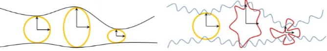
Droplets dispersing in a turbulent flow field are expected to deviate from the trajectories inferred from a certain averaged solution, due to turbulent fluctuations, resulting in a turbulent mixing of droplets as shown in Figure 1. For droplets with large inertia we can assume that large scale eddies (resolved in the filtered flow field) are the main contributors to the momentum transport of droplets (2). The small-scale fluctuations are assumed to contribute only to the transport equation for the droplet number density as discussed in Section 5. Hence, the averaged momentum equation for a sampling droplet can be written as:
dVd
dt =
1 τd
where,Vdis referred to as the ‘filtered’ velocity of the droplet.Vdis defined implicitly as the velocity inferred from
the filtered flow field; it can be multivalued.
When deriving (14) the momentum transport due to the unresolved velocity fluctuations was ignored. Thus,VdiVd j
is considered equal toVdiVd j. Having assumed thatv0d,ivd0,jVd,iVd,jwe treat the system of droplets as a pressureless
continuum. In this case the mean mass velocity coincides with the velocity of a sampling droplet.
Taking into account the contribution of the transport of mass due to fluctuations of droplet velocity induced by the subgrid fluctuations of the carrier phase velocity, Equation (3) can be generalised to:
d dt
Z
VL(t)
nddxd =−
Z
SL(t)
jTdS =−
Z
VL(t)
div(jT)dxd, (15)
whereVLis the Lagrangian volume of the droplet medium moving with the filtered velocityVd,SLis the surface of
this volume, andjT is the additional flux of the droplets due to droplet velocity fluctuations induced by the subgrid
fluctuations of the carrier-phase velocity. This equation is then transferred into the differential form in Lagrangian coordinatesx0, as was done when deriving (6), leading to the following continuity equation for droplets:
d
dtnd(x0,t)||J||=−div(jT)||J||, (16)
where||J|| is the absolute value of the determinant of the Jacobi matrix of the transformation from the Eulerian to Lagrangian coordinates for the droplet medium motion with averaged velocity Vd. This approximate ‘filtered’
description of the droplet motion is valid when the contributions of the droplet velocity fluctuations to the mass
and momentum fluxes are both small, but the ratio|jT|/nd|Vd|is much greater than the ratiov0d,iv0d,j/V
2
d,i. As shown
later with reference to an example of a simple one-dimensional flow, this condition can be satisfied for droplets with moderate inertia (see Section 4).
We assume that Fick’s law is applicable, which allows us to presentjT as:
jT =−DT∇ns, (17)
whereDT is the turbulent diffusion coefficient. Having substituted (17) into (16) we obtain the equation for droplet number density in the form of a modified convective diffusion equation:
d
dt(nd(x0,t)||J||)=div(DT∇nd)||J||. (18)
To estimate the values of the turbulent diffusion coefficient of dropletsDT, we need to know the intensity of the turbulent fluctuations for the droplet velocities along the filtered droplet trajectories. The average energy of these fluctuations can be estimated askv = 0.5·v0·v0, wherev0are fluctuations of the droplet velocities in individual
computational cells. Using the above definition ofkv, the characteristic velocity of droplet fluctuations is estimated as V= √2/3kv.
The turbulent fluxjT is assumed to be driven by Fickian diffusion due to individual droplet fluctuations. Recent
research on the dispersion of particles has highlighted the analogies between particle dispersion in turbulence and Brownian motion (92). The physical mechanism of Brownian motion occurs at the molecular scale and it is different from the mechanism responsible for the oscillation of droplets in a turbulent flow field. The diffusion of droplets in a turbulent field, however, is proportional to the characteristic velocity of their fluctuations, as in Brownian motion (see Section 6). Following (92), the droplet turbulent diffusion coefficient can be presented as:
DT =VL, (19)
whereVandLare characteristic velocity of the turbulent fluctuations and their characteristic length, respectively. The value ofVis calculated as the product of the characteristic velocity of the carrier phaseUand the ratio of V andU : λ = V/U. The carrier phase characteristic velocity stems from the subgrid turbulent kinetic energy
ksgs =0.5u0·u0of the carrier phase fluctuations asU= p2/3ksgs. Coefficientλcan be estimated using the intensity
dV2
dt =
1 3
d dtv
0
iv
0
i =
1 32v
0
i dv0
i
dt =
2 τd
1 3v
0
iu
0
i−
1 3v
0
iv
0
i
!
. (20)
The 13v0iu0iin the expression 20 is the modulation term and expresses the correlation of the dispersed phase fluctu-ationsv0to the fluctuations of the carrier phaseu0
. For droplets with high Stokes numbers St the fluctuations of the carrier phase do not interact with the droplet velocities thus the modulation term is expected to reach zero while for low inertia droplets their that follow the carrier phase fluctuations the modulation term is bounded by an upper limit U2.
The scope of this work is the extension of the FLA for turbulent flows by the introduction of an unresolved exchange of particles across the Lagrangian volume. The complex interaction between the dispersed phase fluctuations and the flow fluctuations of a turbulent carrier phase discussed in (81) was initially investigated by Tchen (85). In this paper, the turbulent diffusion approach has been followed for the evaluation of the turbulent mass flux in Equation 16. According to (96) the algebraic (local equilibrium) models (18, 12, 10) have gained wide acceptance for the calculation of the dispersed phase turbulent characteristics. Within the framework of one of these approaches, the turbulent stresses of the dispersed phase are directly related to the Reynolds stresses of the carrier flow. Following Danon et al. (18) we can write:
1 3v
0
iu
0
i=U
2e−Bτd/τt. (21)
Hence,
dV2
dt =
2 τd
U2e−B
τd
τt − V2
, (22)
whereτtis the characteristic turbulence time.Bis an empirical constant introduced in Danon et al. (18) for the round
jet configuration. Following (11), where local isotropy is assumed, the empirical constantBis taken equal to 0.5 (see Chan et al. (9), Pakhomov and Terekhov (58)). Equation (22) provides the rate of change of the droplet fluctuation intensity accounting for the dynamic response of droplets to the carrier phase turbulent fluctuations. Taking into account that the integral length scale is responsible for the diffusion of the discrete phase, the diffusion coefficient in (19) can be modelled on the integral length scales usingL= ∆andV=λU, as:
DT =λ 2
3ksgs !1/2
∆ . (23)
In our analysis, the standard closure for the subgrid turbulent kinetic energy has been chosen based on the magni-tude of the resolved rate of the strain tensor|S|= p
2Si jSi j:
ksgs =
c4S c2
v
∆2|S|2 , (24)
wherecS is the Smagorinsky constant andcv is assumed to be equal to 0.1 (see Pope (66)). ∆is the length scale inferred from the size of the filtering volumeΩi,∆ = Ω1i/3, providing a measure of the resolved integral length scale.
The theoretical value for the Smagorinsky constant,CS = 0.16, is used in our analysis (see Lilly (44), Clark et al. (15), Kwak et al. (41)).
Integrating (16) over time and taking into account (19) we obtain the following expression for the droplet number density:
nd(x0,t)=
nd(x0,0)+
Rτ=t
τ=0||J(x0, τ)|| ∇ ·(DT∇nd(x0, τ))dτ)
||J(x0,t)||
. (25)
Figure 1: Left:Schematic pattern of the evolution of a droplet cloud element within a filtered flow field.Right:Schematic pattern of the evolution of a droplet cloud element within a turbulent flow field.
.
3.2. Droplets in a one-dimensional standing wave.
To illustrate the applicability of the approximations on which the model described in the previous section was based, we consider droplet dynamics in a one-dimensional oscillating flow (standing wave) with an imposed high-frequency modulation, similar to Knudt’s well-known dusty-gas flow in a tube. Fundamental flow fields, which can be expressed analytically, are widely used for the study of particle clustering as presented by Monchaux et al. (53). A wide range of synthetic flows for both compressible and incompressible configurations, used for the investigation of pattern formation and clustering of particles in turbulent flows, is presented by Gustavsson and Mehlig (33).
We assume that a large number of droplets is suspended in an infinite vertical column of air. The contribution of gravity is ignored. The droplets are initially confined within a segment with length 4L. Introducing the dimensionless distancex, normalised byL, we can write that this segment is confined betweenx=−2, andx=2. We consider the case when a standing wave consisting of two harmonics is sustained within the one-dimensional column. TakingUm
as the velocity scale, the dimensionless velocity of the carrier phaseuis presented as:
u(x,t)=
2
X
i=1
Umisin(ωiπt) sin(kiπx), (26)
wherekiis the wavenumber andωiis the angular frequency of the standing wave assumed to be proportional to the
wavenumber for both harmonics (ωi = 0.1ki); the velocity amplitude for the first harmonic is Um1 = 1, while for
the second oneUm2 =1/k2. The fundamental wavenumberk1 is taken equal to unity, and the wavenumber for the
modulation wave isk2=16.
For Stokes droplets, the time evolution of their trajectoriesx, nondimensionalised byUmandL, is described by the following equation:
¨
xd+ 1
Stxd˙ + 1
Stu(x,t)=0, (27)
where the droplet Stokes number (St) is defined as the ratioτd/τv,τv=L/Um.
For the carrier phase flow field described by (26), the trajectories of the droplets were calculated numerically by integrating Equation (27) forNdroplets. The results of calculations forN=106and St=5 are presented in Figure
-10 -5 0 5 10
0 20 40 60 80 100
x
[image:11.595.137.466.150.333.2]t
Figure 2: Trajectories of individual droplets,xd(t), dispersing due to the carrier phase velocity oscillations.
-1
-0.5
0
0.5
1 -10
-5
0
5
10
u
(a) (b)
Figure 3:Left:Distribution of the carrier phaseu(x,t) velocity for the one-dimensional Knudt’s tube problem, taking into account the contribution of 2 harmonics, att=5.Right:Number densitynddistribution across Knudt’s tube over time for droplets dispersing due to carrier phase velocity
[image:11.595.119.490.452.650.2]-1
-0.5
0
0.5
1 -10
-5
0
5
10
u
[image:12.595.118.492.162.356.2](a) (b)
Figure 4:Left:Distribution of the carrier phaseu(x,t) velocity for the one-dimensional Knudt’s tube problem, taking into account the contribution of 1 harmonic, att=5.Right:Number densitynddistribution across Knudt’s tube over time for droplets dispersing due to carrier phase velocity
oscillations.
[image:12.595.132.428.452.679.2]Let us now consider the droplet dynamics in a single standing wave in a gas flow:
u(x,t)=Um1sin(ω1πt) sin(k1πx). (28)
In what follows we refer to the velocity distribution (28) as the filtered carrier phase flow field.
In Figure 4 the same plots as in Figure 3, but for the case when the standing wave is approximated only by the first harmonic, are presented. Comparing Figure 3 and Figure 4, in both cases (1 and 2 harmonics) we can observe the mixing and un-mixing behaviour of droplets. At the same time, the filtering leads to the smoothing of the wrinkles in the number density induced by the modulation wave compared with the number density distribution in the un-filtered gas flow (2 harmonics). Note that the trajectories shown in Figure 2 for the un-un-filtered gas flow are almost indistinguishable from those inferred from the filtered gas flow (not shown in the paper).
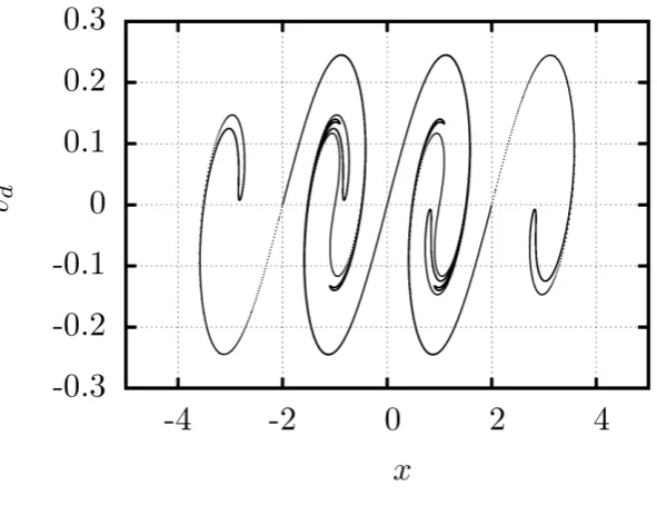
The velocities of the droplets fort =20 for the un-filtered (two harmonics) flow are shown in Figure 5. As can be seen from this figure, the droplet trajectories overlap at some values ofx, leading to multiple velocities for eachx. These overlapping layers can be identified by droplet velocities or their Lagrangian coordinatex0.
In Figures 6(a) and 6(b), the droplet number densities inferred from the FLA, are compared with the number densities inferred from counting the numbers of droplets across 1000 bins (see Figure 3 and 4) for filtered (Figures 6(a)) and un-filtered (Figures 6(b)) carrier phase flows. In the FLA, the number density for each layer is calculated based on continuity equation (6).
In the FLA framework, the droplet number densities in an infinitesimal Eulerian volume nd are inferred from
the Lagrangian number densities. This is achieved by adding the averaged Lagrangian values of the latter for each fold in the droplet cloud found within this volume. This process requires rigorous identification of the folds. This identification is based on a suitably chosen conditioning variablec which can be the droplet velocity, the initial Lagrangian position or the number of changes of the sign of the Jacobian determinant. Conditioning the number density byc, i.e. hnd|cigives the average number density at each fold, while the following integral gives the final value of the number density as predicted by FLA:
nTd =
Z ∞ −∞
hnd|ci
Nfolds
X
i
(δ(c−ci))dc, (29)
where,ciis the value of the conditioning variable at each fold, andδis the Dirac delta function.
The initial Lagrangian position x0 is used as the conditioning variablec. The number densities for each layer,
shown as dashed curves in Figure 6, are summed up. This leads to the total number density inferred from the FLA, shown as circles in the same figure. Four well identified regions where intersection of trajectories occurs can be clearly seen in this figure. In these regions, folds of the dispersed phase are formed resulting in caustic points where droplets accumulate. Here the droplet number densities become very high. This can be clearly predicted by the FLA. In the vicinity of the folds, the results inferred from the FLA, are not close to those inferred from counting the number of droplets at each bin. Although the number densities at caustic points (where the Jacobian is crossing zero) tend to infinity, they are integrable (56). This leads to finite number densities for the specific intervals (bins). For the approach based on box counting of droplets a significant number of individual droplets is needed to achieve accurate estimation of the number densities at the caustic points.
Comparing the plots shown in Figures 6(a) and 6(b), one can see that the number densities predicted for the un-filtered carrier phase flow are much more chaotic than those predicted for the un-filtered flow. Let us now recall that the analysis presented in Section 3 is valid only when the ratio|jT|/(nd|vd|) (normalised turbulent mass flux ˆjT) is much
greater than the ratiov0d,iv0d,j/v2d,i (normalised turbulent momentum flux (pressure) ˆpT). It is not possible to prove
the validity of this condition in the general case. In what follows, however, we will show that it is valid in the case of droplet dynamics in the un-filtered carrier phase flow (two harmonics) when the filtered flow (one harmonic) is considered as a base flow.
The values of ˆjT and ˆpTwere calculated based on the following general expressions:
ˆjT =
|ndgvd| − |ndvdg|
/|ndgvd|, (30)
ˆ
pT =
g
ndv2d−ngdv2d
/ng
10−2
10−1
100
101
-4 -3 -2 -1 0 1 2 3 4
nd
x
10−2
10−1
100
101
-4 -3 -2 -1 0 1 2 3 4
nd
x
[image:14.595.66.459.172.312.2](a) (b)
Figure 6: Droplet number density distributions att =20. Solid red curve: number density calculated by spatially averaging the number of individual droplets across 1000 bins at specific points along thex−axis. Dashed curves: inverse of the determinant of the Jacobi matrix showing the droplet number density at each fold. Circles: number densities obtained by summing up the number densities at each fold.Left:Filtered carrier phase velocity field (one harmonic).Right:Un-filtered carrier phase velocity field (two harmonics).
10−5 10−4 10−3
10−2 10−1
-4 -2 0 2 4
ˆ
pT
,
ˆjT
x
Figure 7: Turbulent momentum flux (pressure), normalised by the resolved momentum fluxndv2d( ˆpT) (thick solid curve), and the turbulent mass
flux, normalised over the resolved mass fluxndvd( ˆjT) (thin solid curve with symbols•) at timet=20 for the droplets dispersing in the un-filtered
[image:14.595.141.458.467.645.2]where operatore· shows averaging over the control volume that corresponds to the wavelength of the second harmonic. The filtering operator·for the droplet velocityvdand the number densityndshow the values inferred from the filtered carrier phase velocity field.
The plots of ˆjT and ˆpTversusxare shown in Figure 7. As can be seen from this figure, ˆpT is generally much (up
to about an order of magnitude) smaller than ˆjT (the cases when both these terms are equal to zero are of no interest
to us) (cf. (2)). This illustrates (but does not prove) the applicability of the condition ˆjT pˆTused in our analysis.
4. The filtered number density and a second order extension of the FLA
In the previous section we presented the formulation of the effect of turbulent diffusion on droplet dispersion in the FLA framework. We demonstrated the implementation of the FLA in an unsteady one-dimensional flow-field and assessed the modelling assumptions for the conservation of mass and momentum. To introduce the FLA in the LES framework, however, the point-wise number density needs to be related to the finite length scale inferred from the LES filter width∆.
In this section we present the second order extension of the FLA showing the spatial structure of the number density field (62). Most importantly the following analysis describes how the FLA approach can model the detailed structure of caustic formations. This is achieved by introducing the second order approximation of the dispersed continuum deformation, the calculation of the filtered number density and finally by the calculation of the Hessian of the transformation of the continuum space in the FLA context.
4.1. The number density in a finite volume
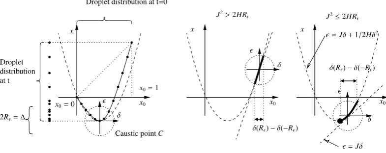
We consider a one-dimensional Stokesian droplet continuum at the locationsxat timestwhich corresponds to its initial distribution at locationsx0which span fromx0 =0 tox0=1 at timet=0 as shown in Figure 8. This continuum
disperses and deforms as shown by the solid curve in Figure 8. Functionx(x0) is uniquely defined atx0. The filtered
number density at any pointCis obtained by spatially averaging the number of droplets within a filtering volume of size∆on thexaxis. We can define the local coordinate systemδ=x0−xC0 and=x−x
Cfor the distribution of the
deformed continuum. The point-wise number densityndat a point0in the local coordinate system is calculated as:
nd(0)=
lim
→0
δ()−δ(−) 2 = ∂δ ∂ = 0 , (32)
where∂∂δ is equal to the JacobianJandnd =1/|J|. Equation 32 can be inferred from the mass conservation 3. IfCis located at a caustic point, where ∂∂δ is zero, then the number density atCis infinitely large. It will be shown later in this section that the number density distribution can be integrable over a finite volume, and a filtered number density ˆ
ndcan be defined and predicted.
Assuming that the number density ∂δ∂ is integrable in the interval0 ∈[−R,R], the spatially averaged or filtered
number density ˆndfor an interval∆ =2Rof the Eulerian spacecan be estimated as:
ˆ
nd= 1
2R
Z R
−R
ndd=
δ(=R)−δ(=−R) 2R , (33)
wherend is evaluated from Equation 32. For the first order FLA, a simple linear expression for the dispersed con-tinuum distribution = Jδis assumed. In this case, Equation 33 leads to the standard first order expression for the filtered number density ˆnd = 1/J. As shown in Figure 8, in the vicinity of a fold the linear approximation for(δ) cannot represent the topology of the fold. We introduce the second order Taylor approximation for(δ) as:
(δ)= ∂ ∂δ δ=0
δ+1
2 ∂2 ∂δ2 δ=0
δ2. (34)
The first derivative ∂∂δ = ∂∂xx
0 in Expression 34 is equal to the JacobianJ, while the second derivative
∂2
∂δ2 =
∂2x
∂x2 0
is
equal to the HessianHof the transformation from the Eulerianxto the Lagrangian coordinatex0at the point =0.
Thus, the approximation of the transformation(δ) (dashed parabola in Figure 8Left) can be presented as:
(δ)=Jδ+1
2Hδ
x
x0
x0=1
δ
Droplet distribution at t=0
x0=0
Droplet distribution at t
Caustic pointC
2R= ∆
x x
δ
δ
x0 x0
J2>2HR
J2≤2HR
=Jδ =Jδ+1/2Hδ2
δ(R)−δ(−R)
[image:16.595.100.493.113.269.2]δ(R)−δ(−R)
Figure 8: Left:Schematic representation of the deformation of the dispersed continuum at the vicinity of a fold. The horizontal axis represents the initial Lagrangian coordinatex0. The vertical axis corresponds to the current Eulerian coordinatexat timet. Straight dotted line: the distribution
x(x0) fort = 0. Solid curve: the distributionx(x0) at timet. Dashed curve: the approximation of the continuum distribution in the second
order FLA. Axesδandcorrespond to the local coordinate system atC. Middle:The position of the filtering interval∆ =2RaroundCwhen
J2 >2RH. Right:The position of the filtering interval∆ =2R aroundCwhenJ2 <2RH. Straight dashed line: the approximation of the continuum distribution in the first order FLA.
We can choose the orientation of the local coordinate systemδ=±(x0−x0C) and=±(x−xC) to ensure that both
HandJare positive. The solution to (35) can be presented as:
δ()= −J+ √
J2+2H
H , (36)
were we have chosen the root closest to the Taylor expansion reference point. We can evaluate Expression (33) for the filtered number density as:
ˆ
nd =
−J+
√
J2+2HR
H −
−J+
√
J2−2HR
H
2R =
2 p
J2+2HR
+pJ2−2HR
, (37)
whenJ2>2HR. ForJ2<2HR, Solution (36) is defined only for=Ras for=−Rthe filtering interval extends outside the fold of the dispersed continuum. In this case the integral in Equation (33) is evaluated only in the interval [min,R].mincorresponds to the minimum limit of the droplet distribution that occurs atδmin=−J/H. Thus, for the
case when JacobianJis small relative to the curvature of the fold, the number density inferred from Equation (33) can be estimated as:
ˆ
nd =
−J+
√
J2+2HR
H +
J H
2R =
p
J2+2HR
2RH , (38)
whenJ2−2HR
<0. As follows from Equation 38, the number density for a caustic pointJ=0 becomes:
ˆ
nd= √ 1
2RH
. (39)
calculated as: ˆ nd= 2 √
J2+2HR+
√
J2−2HR ifJ
2−2HR
>0
√
J2+2HR
2RH ifJ
2−2HR
<0.
(40)
WhenJ2 =2HR
then ˆnd =
√
2/Jfor both the first and second branches of Equation (40). For J2 >>2HR
, where the dispersed phase is diluted, the above expression simplifies to the classical FLA expression ˆnd =1/J.
This model can be applied for multi-dimensional cases taking into account that the local structure of the fold is one-dimensional, i.e. the caustic is a surface in three dimensions or a curve in two dimensions. This can be supported by our findings in Section 5 (cf. Figure 17).
4.2. Calculation of the Hessian
In this section, a method for calculation of the value of the Hessian along a trajectory will be presented. This method is similar to the approach used in the classical FLA for the calculation of the Jacobian. An initial value problem for the time derivative of the Hessian, represented by the auxiliary variableψ, can be formulated by differentiating the equivalent expression forωover the Lagrangian coordinatex0. The derivation of the initial value problem is presented
in the Appendix A. The initial value problem for the calculation of the Hessian and the Jacobian is finally described by the following explicit non-linear differential system of equations:
∂ ∂t J ω H ψ = ω 1 τd ∂U
∂xJ−ω
ψ
1
τd ∂2U
∂x2J
2+∂U
∂xH−ψ
, with J ω H ψ
t=0 = 1 ∂V ∂x 0
∂2V
∂x2
(41)
System (41) will be solved numerically using a fourth order Runge-Kutta method. The same method can be imple-mented for a multi-dimensional case, where each component of the Hessian tensorHk
i j = ∂Uk
∂x0,ix0,j and its equivalent auxiliary variableψk
i j = ∂ ∂tH
k
i jis integrated by the corresponding ODE.
For the results of the second order FLA presented in the next section, the differential system 41 is numerically integrated over time using a fourth order Runge-Kutta method. The same method can be implemented for a multi-dimensional case for finding each component of the Hessian tensorHi jk = ∂xk
∂x0,ix0,j and its equivalent auxiliary variable ψk
i j= ∂ ∂tH
k i j.
4.3. Droplets in a one-dimensional converging flow
In this section we demonstrate the calculation of spatially filtered number densityndwithin a finite volume∆ =2R
using the second order FLA. We compare the second order FLA results with the results inferred from the standard Lagrangian approaches where the number density is calculated by a box counting method. As in the previous one-dimensional numerical simulations, we assume that a large number of droplets is suspended in an infinite vertical column of air. For the dimensionless distancex, normalised byL, the droplets are distributed betweenx=−0.5, and
x=0.5. We assume a simple compressible converging one-dimensional flow fieldu(x) for the carrier phase, described by the following equation:
u(x,t)=−cos(2πx). (42)
The problem is modelled using a standard Lagrangian approach with 106 individual droplets dispersing under the
influence of the carrier phase field using Equations (1) and (2) for Stokes droplets. The Stokes number for this case is assumed equal to St=10.0. The number density for each FLA droplet is calculated using Equation (6) for the first order FLA and Equation (40) for the second order FLA. The Jacobian and the Hessian are calculated using the fourth order Runge-Kutta method for the integration of System (41), as described in the previous section.
−0.4
−0.2
0 0.2 0.4
0 1 2 3 4 5
|J|
xd
t
10−1
100
101
102
103
104
0 1 2 3 4 5
nd
[image:18.595.79.525.114.263.2]t
Figure 9:Left:Trajectories of FLA droplet clouds,xd(t), dispersing in the carrier phase. The circles diameters are proportional to the magnitude
of JacobianJ. Right:Number density ˆndon a single fold along thex0 =−0.25 droplet trajectory assuming an infinitesimally small averaging
volume withR→0.
10−1
100
101
102
103
104
0 1 2 3 4 5
nd
t
10−1
100
101
102
103
104
0 1 2 3 4 5
nd
t
Figure 10:Left:Number density ˆndon a single fold along thex0 =−0.25 droplet trajectory, assuming an averaging volume with 2R =0.001.
Right:Number density ˆndalong thex0=−0.25 droplet trajectory assuming an averaging volume with 2R =0.01. Solid red curve: result from
the second order FLA. Circles: result from box counting on the same length scale. Thin curve: result from the standard FLA.
is proportional to the magnitude of JacobianJ. Small circles indicate high number densities. The Jacobian is zero at the locations where the carrier phase field compresses droplet clouds, resulting in trajectory intersections. The number density of the droplet gradually increases with time as droplets converge into a progressively smaller space. The droplet trajectory x0 = −0.25 highlighted in Figure 9 (Right) will be used as a reference trajectory for the
presentation of the first and second order FLA results.
In Figure 9 (Right) we present the comparison of number densities along a single trajectory using the standard FLA method (or assumingR =0). The result for a single FLA droplet is compared with the result inferred from the box counting Lagrangian method where the minimal box size containing three droplets is used. As can be seen from this figure, the standard FLA approach allows us to predict adequately the droplet number density using a single Lagrangian element. It can be observed, however, that the number densities at the vicinity of the trajectory intersections (att = 1.2 for thex0 = −0.25) reach very high values. The values of these densities vary depending
on the number of droplets used and the temporal resolution and can become infinitely large. In the first order FLA context, the structure of the droplet distribution close to caustics is considered as unresolved at a finite length scale.
In Figure 10 we show the values of the number density as inferred from the second order FLA. In Figure 10 (Left) we show the number density for a filter width equal toR=0.0005, as compared with the predictions of the standard
FLA and the box counting method. The latter usesN =106droplets, assuming an averaging volume∆of the same
[image:18.595.80.525.319.465.2]10
010
110
210
310
40
.
8
0
.
9
1
1
.
1
1
.
2
1
.
3
n
dt
Figure 11: Total number density ˆndalong thex0 =−0.25 droplet trajectory assuming an averaging volume with 2R =0.001. Solid red curve:
result inferred from the second order FLA. Circles: result inferred from box counting on the same length scale. Thin curve: result inferred from the standard FLA.
As can be seen from the figures above, the description of the inner structure of the caustic formations in the second order FLA context results in the accurate prediction of the filtered number density calculated by the box counting Lagrangian simulation. Given that in the vicinity of the trajectory intersections the Hessian of the dispersed continuum distribution is finite, the second order FLA not only results in a finite value fornd, but also provides an accurate prediction of the values of the filtered number density ˆnd(see Appendix B). Of course, in the regions away from caustic formations, the dispersed continuum structure is resolved, and both the standard FLA and the second order FLA give the same predictions. As can be seen in the same Figure 10 (Right), the box counting method shows a discontinuity at the trajectory intersection. This is not observed for the result inferred from the second order FLA. The reason for this behaviour is that the branch of the upwind fold is not symmetric relative to the branch of the downwind fold. This could be modelled by introducing the third order approximation for the distribution of the dispersed continuum. In the immediate vicinity of the caustic, the filtering volume is only partly occupied by droplets. This explains the decrease in the droplet number density observed on the caustic, as shown in the same figure.
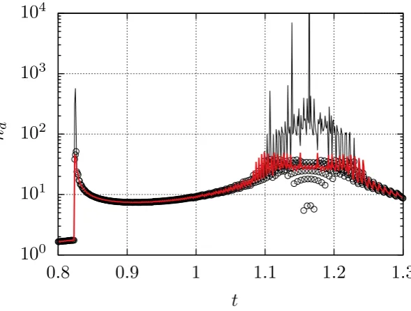
The total number density, calculated for all the trajectories from every fold found within a volume of characteristic length ∆along the path of the x0 = −0.25 droplet, is shown in Figure 11. In order to obtain the total average
number density, the domain−0.5Lto 0.5Lis divided into finite volumes of size∆. For the direct simulation using Lagrangian droplets we count all the droplets within the averaging volume in which the reference droplet is found. The summation of the folds for the standard and the second order FLA approaches is also performed for the same volumes using Equation 29. In Figure 11 we focus on the time intervalt = 0.8 tot = 1.3. In this interval, we observe two regions of high number density. The first consists of a single peak att=0.825 which coincides with the intersection of the reference trajectory with distant trajectories which have formed a caustic. The peak at this point reachesnd =40 as predicted by the second order FLA and the box counting method. The standard FLA provides a spurious (non-converging) prediction ofnd =500. After this peak, the number density remains almost constant with
nd ∼ 10. The second region consists of a series of peaks and coincides with the folding of the reference trajectory itself. In both cases, the second order FLA predicts the filtered number density by modelling the internal structure of the dispersed continuum fold. For the specific filter length∆ =0.001 used in Figure 11, the second order FLA shows peaks of number density that are only 2 to 3 times the number densities away from caustics. This agrees with the direct simulation result.
[image:19.595.163.458.115.338.2]discussed in Section 5, while the second order approach provides a spatially filtered value. The box counting method needs a very large number of droplets to identify the details of the internal structure of the fold even for simple one-or two-dimensional problems. For three-dimensional and/or more complicated problems, a simple Lagrangian approach would require a prohibitive number of droplets for the description of caustics.
5. Droplet mixing in homogeneous and isotropic turbulence
In this section, the model is applied to the analysis of time evolution of the localised droplet distribution in the field of decaying homogeneous and isotropic turbulence of the carrier phase. The Lagrangian approach is used to show the structure of the dispersed phase distribution under the influence of a complex turbulent flow field characterised by detailed simulations with an order of 108degrees of freedom. The Lagrangian methods based on the statistical
properties of a large number of droplets would require a computationally prohibitive number of individual droplets (as demonstrated in the simple one-dimensional fields) to resolve the complex fine scale of the dispersed continuum structure. Thus, statistical analysis of simple Lagrangian droplets for this family of problems is used only for the assessment of the turbulent diffusion problem.
5.1. Numerical method: The solution and the initialisation of the carrier phase DNS
The turbulent mixing of droplets is investigated using numerical experiments on homogeneous and isotropic tur-bulence. The evolution of the turbulent flow field is governed by the incompressible Navier-Stokes (NS) equations. The solution for the turbulent flow field is inferred from the numerical integration of the NS equations for the vorticity
ω=∇ ×U:
∂U
∂t =U×ω− ∇Π +
1 Re∇
2U, (43)
∇2Π =∇(U×ω), (44)
where Re is the Reynolds number (all variables in this section are dimensionless) andΠis the total pressure:
Π = p+1
2|U|
2. (45)
Equation (43) is solved using the pseudo-spectral method derived by Rogallo (73) in its parallel implementation as described by Papoutsakis (61). This code is based on the code originally developed by Kerr (40).
The computational domain, used in our analysis, is a cube with sizeL =2πwith periodic boundary conditions in all three directions. Equation (43) is integrated in the spectral space. It is necessary to calculate the non-linear termU×ωin the physical space. One Real Fast Fourier Transform (RFFT) and two Complex FFTs (CFFT) are applied in order to obtainU×ωin the spectral space. The alias errors occurring during the Fourier transformations are removed using the 2/3 rule (the high wavenumber part of the spectrum is ignored) Kerr (40). The initial value problem described by Eqs. (43) and (44) is integrated over time using the minimal storage time-advancement third order Runge-Kutta scheme developed by Alan Wray as described in Kerr (40). In this algorithm, three realisations of the flow field at three equivalent intermediate time steps are used to provide the final prediction.
Simulations of turbulent flow fields are based on taking into account all the scales of turbulent fluctuations. One of the conditions for the full resolution of a turbulent flow field stems from the requirement that the dissipation spectrum must be resolved. For any pseudospectral implementation, this restriction is described as Pope (66):
∆x< 2π
3 η , (46)
where∆x=2π/NDNSis the spatial resolution of the solution.
Number of nodes N 2563
Spatial resolution ∆x 0.025
Reynolds number Re 200
t=0 t=2
Turbulent kinetic energy kt 1.57 0.66
Kolmogorov length scale η 0.0214 0.0257
Kolmogorov time scale τη 0.0922 0.1325
Taylor microscale λT 0.366 0.314
Taylor Reynolds number ReT 74.8 45.4
Integral length scale L 1.03 0.95
Integral time scale τt 1.02 1.43
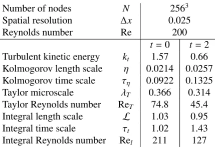
[image:21.595.190.405.108.256.2]Integral Reynolds number Rel 211 127
Table 1: Non-dimensional parameters for the Direct Numerical Simulation of homogeneous and isotropic turbulence, att=0 and att=2.
superposition of Fourier modes. The intensity of each Fourier mode is initialised using the energy spectrumE(|k|) provided by Orszag and Patterson (55):
E(|k|)=c|k|4e−|k|2/a2 , (47)
wherekis the wavenumber vector for each mode. Constantscanda are chosen in such a way that all scales of the resulting turbulent flow field are well resolved (see Mell et al. (50)). The phases for each of the Fourier modes are chosen randomly, subject to consistency with the mass conservation equation (see Hussaini and Zang (37)). The synthetic turbulent flow field stemming from (47) does not have a developed dissipation spectrum and does not lead to correct high order velocity correlations (see Kerr (40)).
In order to obtain a homogeneous isotropic turbulent flow field, the initial synthetic field is integrated over time, while the energy of the large eddies is maintained by forcing. Forcing mimics the energy cascade from larger to smaller scales observed in turbulent flows. This maintains the kinetic energy of the turbulent flow field during its integration and avoids its decay due to viscosity. In the current implementation, the forcing is achieved by artificially increasing the energy of the fluctuations for the two lowest wavenumbers with|k| = 1 and|k| = 2 when the total turbulent kinetic energy becomes smaller than its initial value. This forcing is applied until the turbulence statistics of the flow converge to a constant value. At this stage a developed turbulent flow field was obtained and used as an initial condition for the numerical experiments of droplet dispersion.
The details of the calculated turbulent flow field are summarised in Table 1. Mesh resolution ofN=2563nodes
was used. This allows adequate resolution of the dissipation spectra of the simulations of homogeneous and isotropic turbulence. The resulting flow field is characterised by a Reynolds number (based on the Taylor microscaleλT and
the characteristic velocityU) equal to ReT = 74.8. The definition of the Taylor microscale is based on the two
point velocity correlation coefficient. It is calculated from the carrier phase turbulent kinetic energy (3/2)U2and the dissipation rateas:
λT =
r
15νU
2
, (48)
whereU2andwere evaluated from the DNS data.
5.2. Numerical method: The solution and the initialisation of the dispersed phase
calculated from (14). For the Fully Lagrangian Approach (FLA) calculations, the elements of the Jacobian matrix and the corresponding auxiliary variable matrix are also obtained using (10) and (11) for each sampling droplet. The corresponding equations are solved using the same third order Runge-Kutta scheme. The interactions between droplets and the effect of droplets on the carrier phase are ignored assuming low mass load of the dispersed phase.
During the first stages of the numerical experiment, the droplets are expected to adapt to the fluctuations of the carrier phase flow field. To reduce this adaptation stage, droplet velocities are initialised by the asymptotic values given by (22):
Vi(t=0)=e12
−Bτd
τt
Ui(t=0) . (49)
Following Lebedeva et al. (43), the elements of the Jacobi matrixJi jand matrixωi jin (10) and (11) are initialised
as:
Ji j(t=0)=δi j, ωi j(t=0)= ∂Vi
∂xj , (50)
whereδi jis the Kronecker delta.
To verify the predictions of the model we compared the filtered number densities of droplets, inferred from the exact DNS solution, and the number densities for sampling droplets inferred from our model, using the filtered DNS solution.
The topology of the numerical experiments is presented in Figure 12. The computational domain with sizeL=2π is divided intoNLES3 volumes with filter width equal to∆ = 2π
NLES. The DNS solutionU(x,t) is filtered in space using
the box filtering operator·described by (13). Thus, the filtered flow fieldU(x,t) is obtained.
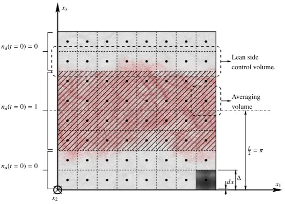
The test case used as a benchmark for our investigation is the diffusion of droplets initially arranged in a slab formation as shown in Figure 12. A uniform distribution of sample droplets was assumed, with the droplets scattered across the computational domain. The diffusion of droplets to the areas away from the initial concentration of droplets is considered. The sample droplets within the slab region were initialised with number densitynd =1, whereas the sample droplets in the areas where the number density of individual droplets is zero are initialised withnd =0. This initialisation is summarised as:
nd(x,0)=
1, if |x3−π| ≤π/2
0, otherwise , (51)
and is used as a benchmark set-up for the assessment of the performance of our model in predicting the mixing of droplets from the rich region to the lean region as shown in Figure 12. The rich region is shown as the red coloured sample droplets along the centreline of this figure, while the lean region is shown as the grey coloured sample droplets in the same figure. The initially segregated droplets are expected to mix due to the effect of the turbulent flow field. Two sets of sample droplets were allowed to disperse. The first set ofNdDNSsample droplets is allowed to disperse along the trajectoriesxDNSd , inferred from exact DNS solutionU(x,t) for the turbulent flow field. The second set of
NdLESsample droplets, is initialised in the same way as the first one. It is allowed to disperse on the filtered turbulent flow fieldU(x,t) resulting in a different set of trajectoriesxLESd .
Three simulations with Stokes numbers St=0.01, St=0.1 and St=1.0 were carried out. The input parameters are shown in Table 2. Two levels of resolution (∆ = 24π and∆ = 28π), usingNLES=4 andNLES=8 averaging volumes,
were used: the coarse mesh withL/∆ =0.66, whereL/∆is the ratio of the integral scale to the filter width, and the fine mesh withL/∆ =1.31.
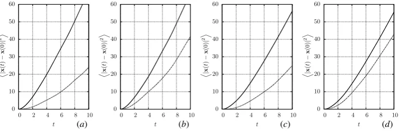
5.3. Results: An analogy between Brownian motion and turbulent diffusion
In Figure 13 we present the temporal evolution of the ensemble averaged squared displacement for DNS droplets D
|xDNS
d (t)−x
DNS
d (t=0)|
2E
and the displacement D|xLES
d (t)−x
LES
d (t=0)|
2E
∆ nd(t=0)=0
nd(t=0)=0
Lean side control volume.
Averaging volume
L
2=π
nd(t=0)=1
dx x
1
x2
[image:23.595.155.433.178.377.2]x3
Figure 12: Topology of the numerical experiment. Red dots: sample droplets withnd(t=0)=1. Grey dots: sample droplets withnd(t=0)=0.
An example of the DNS mesh is shown in the bottom right corner. Thex2axis is directed into the page as indicated in the bottom left corner of the
figure.
Stokes number
St=τp/τ0 St=0.01 St=0.1 St=1.0
Kolmogorov scale Stokes number
St=τp/τη Stη=0.467 Stη=4.67 Stη=46.7
Equilibrium characteristic velocity ratio λin f =e
1 2
−Bτd
τt
0.997 0.975 0.778