City, University of London Institutional Repository
Citation
:
Chugh, S., Ghosh, S. ORCID: 0000-0002-1992-2289, Gulistan, A. and Rahman,
B. M. A. (2019). Machine Learning Regression Approach to the Nanophotonic Waveguide
Analyses. Journal of Lightwave Technology, doi: 10.1109/jlt.2019.2946572
This is the accepted version of the paper.
This version of the publication may differ from the final published
version.
Permanent repository link:
http://openaccess.city.ac.uk/id/eprint/23035/
Link to published version
:
http://dx.doi.org/10.1109/jlt.2019.2946572
Copyright and reuse:
City Research Online aims to make research
outputs of City, University of London available to a wider audience.
Copyright and Moral Rights remain with the author(s) and/or copyright
holders. URLs from City Research Online may be freely distributed and
linked to.
City Research Online:
http://openaccess.city.ac.uk/
[email protected]
1
Machine Learning Regression Approach to the
Nanophotonic Waveguide Analyses
Sunny Chugh*, Souvik Ghosh, Aamir Gulistan and B. M. A. Rahman,
Life Fellow, IEEE
Abstract
—Machine learning is an application of artificial
intel-ligence that focuses on the development of computer algorithms
which learn automatically by extracting patterns from the data
provided. Machine learning techniques can be efficiently used for
a problem with a large number of parameters to be optimized
and also where it is infeasible to develop an algorithm of specific
instructions for performing the task. Here, we combine the finite
element simulations and machine learning techniques for the
prediction of mode effective indices, power confinement and
coupling length of different integrated photonics devices. Initially,
we prepare a dataset using COMSOL Multiphysics and then this
data is used for training while optimizing various parameters of
the machine learning model. Waveguide width, height, operating
wavelength, and other device dimensions are varied to record
different modal solution parameters. A detailed study has been
carried out for a slot waveguide structure to evaluate different
machine learning model parameters including number of layers,
number of nodes, choice of activation functions, and others.
After training, this model is used to predict the outputs for
new input device specifications. This method predicts the output
for different device parameters faster than direct numerical
simulation techniques. Absolute percentage error of less than
5% in predicting an output has been obtained for slot, strip and
directional waveguide coupler designs. This study pave the step
towards using machine learning based optimization techniques
for integrated silicon photonics devices.
Index Terms
—Machine learning, neural networks, regression,
multilayer perceptron, silicon photonics.
I. I
NTRODUCTION
M
ACHINE learning (ML) technology is being
exten-sively used in many aspects of modern society:
web searches, social networking, smartphones, bioinformatics,
robotics, chatbots, and self-driving cars [1]. ML techniques
are used to classify or detect objects in images, speech to text
conversion, pattern recognition, natural language processing,
sentiment analysis and recommendations of products/movies
for users based on their search preferences. ML algorithms can
be trained to perform exceptionally well when it is difficult
to analyze the underlying physics and mathematics of the
problem [2]. ML algorithms extract patterns from the raw
data provided during the training without being explicitly
programmed. The learned patterns can be used to make
predictions on some other data of interest. ML systems can
be trained more efficiently when massive amount of data is
present [3], [4].
Recently, research on the application of ML techniques for
optical communication systems and nanophotonic devices is
*Corresponding author: [email protected]
Sunny Chugh, Souvik Ghosh, Aamir Gulistan and B. M. A. Rahman are
with the School of Mathematics, Computer Science & Engineering, City,
University of London, London, EC1V 0HB, U.K.
gaining popularity. Several developments in ML over the past
few years has motivated the researchers to explore its potential
in the field of photonics, including multimode fibers [5],
power splitter [6], plasmonics [7], grating coupler [8], photonic
crystals [9], [10], metamaterials [11], photonic modes fields
distribution [12], label-free cell classification [13], molecular
biosensing [14], optical communications [15], [16] and
net-working [17], [18].
Complex nanophotonic structures are being designed and
fabricated to enable novel applications in optics and integrated
photonics. Such nanostructures comprise of a large number of
parameters which needs to be optimized for efficient
perfor-mance of the device and can be computationally expensive.
For example, finite-difference time-domain (FDTD) method
may require several minutes to hours to analyze the optical
transmission response of a single photonic device depending
on its design. ML approach offers a path for quick estimation
of the optimized parameters for the design of complex
nanos-tructures, which are critical for many sensing and integrated
optics applications.
ML algorithm considers general function approximations to
learn a complex mapping from the input to the output space.
The most popular ML frameworks for building and training
neural networks includes SciPy [19], Scikit-learn [20], Caffe
[21], Keras [22], TensorFlow [23] and PyTorch [24]. PyTorch
makes use of tensors for training neural networks along with
strong GPU acceleration. It provides separate modules to build
a neural network and automatically calculates gradients for
backpropagation [25] that are required during the training of
a neural network. PyTorch appears to be more flexible with
Python and NumPy/SciPy stack compared to TensorFlow and
other frameworks, which allows easy usage of popular libraries
and packages to write neural network layers in Python.
Scikit-learn is another simple and efficient ML library used for
data mining and data analysis. In our implementation, we use
PyTorch and Scikit-learn numerical computing environment to
handle the front-end modeling and COMSOL Multiphysics for
the back-end data acquisition.
Modeled waveguide designs considered in this paper are
shown in Section II. Main concepts of ML related to integrated
photonics applications are discussed in Section III. In Section
IV, results from ML algorithms using PyTorch and
Scikit-learn with FEM results for commonly used silicon photonic
waveguides and devices are compared, and finally the paper
is concluded in Section V.
II. M
ODELED
W
AVEGUIDES
de-(a)
(b)
[image:3.612.47.300.55.258.2](c)
(d)
Fig. 1: An example of a (a) Slot waveguide showing
E
xfield profile, (b)
Strip waveguide showing
H
yfield profile, and Directional coupler showing
H
yfield profile for (c) even supermode, and (d) odd supermode.
signs: slot waveguide, strip waveguide, and directional coupler.
Cross-sectional view of these waveguides, along with their
respective field profiles are shown in Fig. 1. A range of
slot waveguides (Fig. 1a) and directional couplers (Figs. 1c
and 1d) are simulated by changing the width, height, and
gap between the silicon waveguides as the input parameters.
Effective index and power confinement values are recorded
for slot waveguides, while coupling length was obtained for
directional coupler, corresponding to above mentioned input
parameters. For strip waveguide (Fig. 1b), width, height of
waveguides and wavelength are taken as input variables, while
effective index is considered as the output variable. The
com-mercial 2D FEM software such as COMSOL Multiphysics and
Lumerical can provide the modal solution of any waveguide
within a few minutes. However, a rigorous optimization of the
waveguide design parameters through parameter sweep often
becomes intensive for a modern workstation depending on
the complexity of a design. In this case, we are proposing
an in-house developed ML-algorithm as a stepping stone
for the multi-parameter optimization process where only the
algorithm training (one time process) requires a few minutes
of computational time to learn the features of similar types of
waveguides.
III. N
EURAL
N
ETWORK
T
RAINING
The most common form of machine learning is supervised
learning in which the training dataset consists of pairs of inputs
and desired outputs, which are analyzed by ML algorithm to
produce an inferred function. It is then used to obtain output
values corresponding to any unknown input data samples.
Supervised learning can be further categorised into a
classifi-cation or regression problem, depending on whether the output
variables have discrete or continuous values, respectively. In
this paper, we considered the output predictions of different
integrated photonics structures as a regression problem.
A. Artificial Neural Network (ANN)
Fig. 2: General artificial neural network (ANN) representation, i.e. one input
layer, two hidden layers, and one output layer.
ANN consists of a network of nodes, also called as neurons.
ANN is a framework which is used to process complex data
inputs and it learns from the specific input data without
being programmed using any task-specific rules. One of the
commonly used ANN is the multilayer perceptron (MLP).
MLP consists of three or more number of layers. Here, in
Fig. 2, we have shown a MLP with four layers of nodes: an
input layer, two hidden layers and an output layer. These layers
operate as fully connected layers, which means each node in
one layer is connected to each node in the next layer. All the
nodes have a variable weight assigned as an input which are
linearly combined (or summed together) and passed through
an activation function to obtain the output of that particular
node.
B. Algorithm of ANN
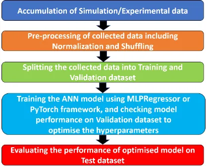
[image:3.612.321.552.84.212.2]The training procedure is illustrated in Fig. 3. Firstly,
suffi-cient number of randomly generated data samples are collected
from the simulations using COMSOL Multiphysics for slot,
strip and directional coupler structures. Each case has an array
of inputs, called features, and an array of numerically solved
outputs, called labels. Waveguide width, height, material, gap
between the waveguides, and operating wavelength values
can be taken as the input variables which are assigned to
Fig. 3: The flow chart of ANN implementation.
[image:3.612.333.543.558.726.2]the nodes of the input layer. Effective index (
n
ef f
), power
confinement (
P
conf
), or coupling length (
L
c
) are taken as
the output variables, which are assigned to nodes of the
output layer depending on the specific design requirement.
Next, preprocessing of the collected data is carried out by
normalizing the input variables values between the range 0–
1 to use a common scale. This is followed by shuffling of
the normalized input data, otherwise the model can be biased
towards particular input data values. Next step is to split the
normalised input dataset into training and validation dataset.
Validation dataset is used to provide an unbiased evaluation of
a model fit on the training dataset while tuning various model
parameters, also called as hyperparameters. 5–25% of data has
been allocated for the validation dataset in this paper, while
the rest was used for training the ANN model.
Neural networks have a tendency to closely or exactly fit a
particular set of data during training, but may fail to predict
the future observations reliably, which is known as overfitting.
During overfitting, the model learns both the real and noisy
data, which negatively impacts on new data. We can avoid
overfitting through regularization such as dropout [26], while
regularly monitoring the performance of the model during
training on the generated validation dataset. Underfitting can
be another cause for the poor performance of ANN model in
which the trained model neither closely fits the initial data
nor generalize to the new data. Hyperparameters needs to
be tuned to reduce the mean squared error (
mse
) between
the actual and predicted output values of the ANN model
for a regression problem. During this optimization process,
weights and biases of the model are repeatedly updated with
each iteration or epoch using the backpropagation algorithm
[25]. Various hyperparameters of choice includes activation
functions, type of optimizer, number of hidden layers, number
of nodes in each hidden layer, learning rate, number of epochs,
and others.
1) Activation Functions:
ANN connects inputs and outputs
through a set of non-linear functions, which is approximated
by using non-linear activation function. Sigmoid, Tanh
(hy-perbolic tangent), and ReLU (rectified linear unit) are few
commonly used activation functions [2].
Sigmoid :
σ
(
z
) =
1
1 +
e
−
z
(1)
Hyperbolic Tangent (Tanh) :
σ
(
z
) =
e
z
−
e
−
z
e
z
+
e
−
z
(2)
Rectified Linear Unit (ReLU) :
σ
(
z
) =
max
(0
, z
)
(3)
Among these, ReLU is used mostly as it trains the model
several times faster in comparison to when using Tanh
func-tion, as discussed in [27].
2) Optimization Solvers:
LBFGS, stochastic gradient
de-scent (SGD), and Adam [28] solvers can be used to optimize
the weights values during ML training process. Adam
opti-mizer is a preferable choice as it works well on relatively
large datasets.
3) Hidden Layers and Nodes:
Number of layers or number
of nodes in each layer of an ANN are decided by
experimenta-tion and from the prior experience of similar problems. There
is no fixed rule to pre-decide their optimal values.
4) Learning Rate:
Learning rate decides how much we
are adjusting the weights of our network with each epoch or
iteration. Choosing the lower value of learning rate means the
model needs more epochs and longer time to converge. If the
input dataset is big, it may take very long time to optimize the
ANN model. On the other hand, if the learning rate has a large
value, then the model might fail to converge at all with gradient
descent [29], [30] overshooting the global minima. Learning
rate can be chosen to have constant or adaptive value when
using Scikit-learn MLPRegressor.
5) Epochs:
Number of epochs to train a model should be
decided by the user when
mse
value converges to acceptable
lower limit. Depending on the dataset size, model training can
be carried out using batches of inputs. In our case, when using
MLPRegressor, we have used automatic batch size, while all
the inputs are trained in one batch with PyTorch.
Once the optimal hyperparameters are obtained, the final
step is to evaluate the performance of optimized trained model
on the previously unseen test dataset (generated separately
from the initially generated dataset) to observe the accuracy
of the ANN model.
IV. N
UMERICAL
R
ESULTS AND
D
ISCUSSION
A. Slot Waveguide
Slot waveguide design structures are extensively being used
for optical sensing applications [31], as the light is confined
in low refractive index region, which allows strong interaction
with the analyte leading to a large waveguide sensitivity.
Here, we demonstrate the use of ML algorithms to predict
the effective index (
n
ef f
) and power confinement (
P
conf
) in
a slot waveguide design [32], but first we optimize the various
hyperparameters of the ANN model.
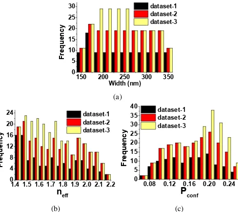
1) Histogram of Datasets:
The training process requires a
dataset of examples, which plays a crucial role in any ML
algorithm. The accuracy of the trained model depends on the
quality of the input data. A good training dataset which is well
aligned with the problem to be solved is needed for ML to
work properly. We have collected 3 different datasets to predict
effective index (
n
ef f
) and power confinement (
P
conf
) for a
slot waveguide structure, shown in Fig. 4. Width, height, and
gap between the waveguides in a slot waveguide design have
been varied initially to record the
n
ef f
and
P
conf
values for
each dataset.
n
ef f
and
P
conf
values recorded for a particular
1 5 0
2 0 0
2 5 0
3 0 0
3 5 0
0
5
1 0
1 5
2 0
2 5
3 0
Fr
eq
ue
nc
y
W i d t h ( n m )
d a t a s e t - 1
d a t a s e t - 2
d a t a s e t - 3
(a)
1 . 4 1 . 5 1 . 6 1 . 7 1 . 8 1 . 9 2 . 0 2 . 1 2 . 2
0
4
8
1 2
1 6
2 0
2 4
Fr
eq
ue
nc
y
n
e f fd a t a s e t - 1
d a t a s e t - 2
d a t a s e t - 3
(b)
0 . 0 8
0 . 1 2
0 . 1 6
0 . 2 0
0 . 2 4
0
5
1 0
1 5
2 0
2 5
3 0
3 5
4 0
Fr
eq
ue
nc
y
P
c o n fd a t a s e t - 1
d a t a s e t - 2
d a t a s e t - 3
[image:5.612.54.298.54.271.2](c)
Fig. 4: Histogram of different datasets for slot waveguide with varying (a)
width of waveguides, (b)
n
ef f, and (c)
P
conf.
3 datasets. For our simulation setup, it took 2-3 minutes to
record one datapoint, which means it took approximately 200,
400, 500 minutes to obtain dataset-1, dataset-2, and dataset-3,
respectively. The time needed to collect one datapoint value
may vary depending on the simulation/experimental setup.
2) Mean Squared Error:
Mean squared error (
mse
) is
considered as the loss function in a regression problem, which
is defined as the average squared difference between the
estimated and true values, given as:
mse
=
1
N
N
X
i
=1
(
y
b
i
−
y
i
)
2
(4)
where
y
b
i
and
y
i
are the estimated and true data point values,
respectively.
Smaller value of
mse
means the predicted regression values
are closer to the original values and hence the model is
well trained. Next, we compare the
mse
values to predict
the
n
ef f
for a slot waveguide design with different number
of nodes or layers in an ANN model for dataset-3 using
MLPRegressor from Scikit-learn. We have chosen dataset-3
0 1000 2000 3000 4000
0.0 0.1 0.2 0.3 0.4 0.5 0.6
M
e
a
n
S
q
u
a
r
e
d
E
r
r
o
r
(
m
s
e
)
Epochs nodes - 05
nodes - 10
nodes - 25
nodes - 50
(a)
0 1000 2000 3000 4000
0.00 0.02 0.04 0.06 0.08 0.10 0.12 0.14
M
e
a
n
S
q
u
a
r
e
d
E
r
r
o
r
(
m
s
e
)
Epochs layers - 1
layers - 2
layers - 3
[image:5.612.51.297.598.711.2](b)
Fig. 5: Mean squared error (
mse
) using training dataset-3 for (a) different
number of nodes with 2 hidden layers, (b) different number of hidden layers
with 50 nodes in each hidden layer.
as it has the maximum number of data points among the 3
datasets generated. Figure 5a shows that
mse
decreases faster
to a stable value when number of nodes is larger.
mse
for
nodes = 50 quickly reaches a stable low value of 0.0025 at
epochs = 1500, shown by a orange line in comparison to
0.0192, 0.0820, and 0.3954 when nodes are taken as 25, 10
and 5, respectively. Random weights are assigned at the start
of the algorithm, hence
mse
for more number of nodes at
first epoch can be larger than that for less number of nodes,
as can be seen from blue and red lines having values of 0.2112
and 0.1423 at first epoch, respectively. It can also be observed
from red and blue lines that model with more number of nodes
attains optimal updated weights quickly than those with lower
number of nodes, as
mse
for nodes = 25 (blue line) decreases
quickly. We run the simulations till 4000 epochs so as to be
sure that
mse
decreases to a lower value. At epochs = 4000,
mse
values are 0.21279, 0.04685, 0.00109, and 0.00018 when
number of nodes are 5, 10, 25, and 50, respectively. This shows
that more neurons/nodes helps is achieving better accuracy for
the ANN model by quickly decreasing the
mse
value to the
minimum, but the computational loading also increases.
Next, we consider the
mse
variations when number of
layers are varied in an ANN model having 50 nodes in each
layer, as shown in Fig. 5b. The
mse
values of 0.0025 and
0.0006 are obtained for models with 2 and 3 number of layers,
respectively at epochs = 1500 in comparison to 0.0243 when
number of layers is equal to 1. Lower stable
mse
values
at epochs = 4000 are 0.00412, 0.00018, and 0.00009 when
number of layers are 1, 2 and 3, respectively, with each layer
having 50 nodes. Following this study, we have considered the
number of layers as 2 with 50 nodes in each layer for future
optimization, to avoid more computational loading compared
to if number of layers were chosen as 3.
3) Activation Functions:
Sigmoid, Tanh and ReLU
activa-tion funcactiva-tions are tested to predict the
n
ef f
and
P
conf
using
MLPRegressor trained model with 2 layers having 50 nodes
in each layer. Dataset-3 is used during the training process.
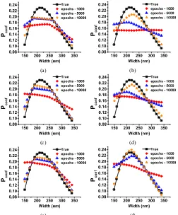
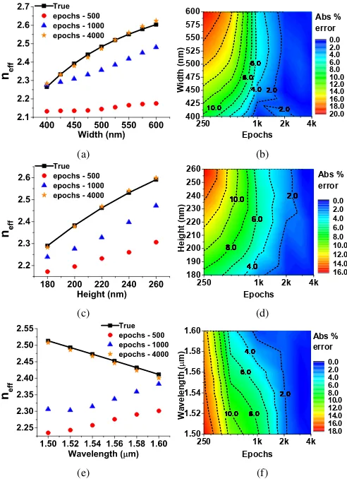
It can be seen from Fig. 6a that Tanh and ReLU are closely
predicting the
n
ef f
values to the true values at waveguide
height = 225 nm of the slot design. Data corresponding to
waveguide height = 225 nm was never recorded or provided
during the training of the model. However, data for other
waveguide heights were used for the training. On the other
hand, Sigmoid function is predicting almost a horizontal line
150 200 250 300 350 1.3
1.4 1.5 1.6 1.7 1.8 1.9 2.0 2.1 2.2
n
e
f
f
Width (nm) True Sigmoid Tanh ReLU
(a)
150 200 250 300 350 0.08
0.10 0.12 0.14 0.16 0.18 0.20 0.22 0.24 0.26
P
c
o
n
f
Width (nm) True Sigmoid Tanh ReLU