http://eprints.whiterose.ac.uk/147065/
Version: Accepted Version
Article:
Maryopi, Dick, Bashar, Manijeh and Burr, Alister Graham orcid.org/0000-0001-6435-3962
(2019) On The Uplink Throughput of Zero-Forcing in Cell-Free Massive MIMO with Coarse
Quantization. IEEE Transactions on Vehicular Technology. pp. 1-5. ISSN 0018-9545
https://doi.org/10.1109/TVT.2019.2920070
[email protected] https://eprints.whiterose.ac.uk/
Reuse
Items deposited in White Rose Research Online are protected by copyright, with all rights reserved unless indicated otherwise. They may be downloaded and/or printed for private study, or other acts as permitted by national copyright laws. The publisher or other rights holders may allow further reproduction and re-use of the full text version. This is indicated by the licence information on the White Rose Research Online record for the item.
Takedown
If you consider content in White Rose Research Online to be in breach of UK law, please notify us by
On The Uplink Throughput of Zero-Forcing in
Cell-Free Massive MIMO with Coarse Quantization
Dick Maryopi, Manijeh Bashar and Alister Burr
Abstract—The recently proposed Cell-Free massive MIMO architecture is studied for the uplink. In contrast to most previous works, joint detection is performed using global CSI. Therefore, we study strategies for transferring CSI to the CPU taking into account the fronthaul capacity which limits CSI quantization. Two strategies for pilot-based CSI acquisition are considered:
estimate-and-quantizeandquantize-and-estimate. These are anal-ysed using the Bussgang decomposition. For a given quantization constraint for the data and CSI the achievable rate per user with Zero-Forcing is determined. Numerical results show that quantize-and-estimate (the simpler strategy) is similar to or better than estimate-and-quantize at low resolution, especially for 1-bit.
Index Terms—Cell-Free Massive MIMO, Fronthaul, Quanti-zation, Bussgang, Channel Estimation.
I. INTRODUCTION
T
HE next generation of wireless networks (including 5G) will be required to provide a high capacity per user and per unit area due to the increasing number of users and the variety of applications expected in the near future. Cell-free massive Multiple Input Multiple Output (MIMO) has been gaining more attention recently as it has the potential to meet this demand [1]. It can be regarded as a form of network MIMO which makes use of a large number of distributed antennas, referred to Access Points (AP), spread over a large coverage area. The term "cell-free" was motivated by the notion of blurring the role of cells so that all users can be served by all APs over the same resources using network MIMO techniques to avoid mutual interference. Because a large number of APs serve a smaller number of users, it still benefits fromchannel hardeningas in co-located massive MIMO [2].Nevertheless, the joint transmission/detection in the most current cell-free system is based only on local Channel State Information (CSI). We identify this a limitation, since relying on local CSI at the APs restricts the feasible choice of process-ing to conjugate beamformprocess-ing or Maximum Ratio Combinprocess-ing (MRC). Other forms of processing such as Zero Forcing (ZF) could be performed at Central Processing Unit (CPU), but would require additional CSI transfer via the fronthaul. However, CF-massive MIMO already faces the problem of high fronthaul load requirement. To address these issues, we study in this paper joint detection with global CSI at the CPU
Copyright (c) 2015 IEEE. Personal use of this material is permitted. However, permission to use this material for any other purposes must be obtained from the IEEE by sending a request to [email protected]. The authors are with the Department of Electronic Engineering, University of York, Heslington, York, UK. email: [email protected]. The paper was supported by Indonesia Endowment Fund for Education (LPDP) and in part by the European Horizon 2020 Programme under GA H2020-MSCA-ITN-2016-722788
and the strategy of acquiring the required CSI. To deal with the growth of fronthaul load we assume a coarse quantization constraint, which is also of interest for the low-cost implemen-tation of APs. We show that using appropriate CSI acquisition strategies, much improved detection techniques can be applied at the CPU resulting in a significant rate improvement in uplink. In [3], a performance improvement of ZF over MRC has also been shown in downlink where a sort of global CSI is used at the CPU for precoding. Nevertheless, they didn’t address specifically the CSI acquisition schemes and the limited fronthaul capacity.
After a brief description of our system model we investigate two strategies of CSI acquisition. The first is called estimate-and-quantize (EQ) where channel estimation is carried out at the AP. The channel estimate is quantized and then the quantized form is sent to the CPU. This is similar to the sharing of quantized CSI between the base stations in the coordinated multipoint (CoMP) scheme [4]. As alternative we considerquantize-and-estimate(QE), where the APs quantize the received pilot and send it to the CPU. From these quantized received pilots the CPU performs the channel estimation. Fur-ther, we compare their performance and their corresponding throughput for ZF detection. Surprisingly enough, the QE strategy, which is simpler for the implementation at the AP, has good performance and a significant performance improvement over EQ for 1-bit fronthaul resolution. Overall, the superiority of utilizing global CSI, even with coarse quantization, is shown to be significant compared to utilizing only local CSI with infinite resolution.
Notation: Roman letters, lower-case boldface letters and upper-case boldface letters are used respectively to denote scalars, column vectors and matrices. The set of all complex and realM×Nmatrices are represented byRM×N andCM×N respectively. The real part and imaginary part of complex numbers are expressed respectively by Re{·} andIm{x}. By
h·,·iwe denote the inner product withk·kas its corresponding vector norm or Frobenius norm. The expectation of random variables is represented byE{·}. We denote the circularly com-plex Gaussian distribution with zero mean and unit variance by CN(0,1). We use IK for the K×K identity matrix and 1K for all-one vector of dimensionK. For a vectora, diag(a)
denotes a diagonal matrix with the diagonal elements taken from vector a.
II. SYSTEMMODEL
the CPU, where the communication between them occurs in baseband form. We assume that the fronthaul link connecting them-th AP with the CPU can in practice transmit reliably at a maximum rate ofRm.
A. Channel Model
The channel between thek-th user and them-th AP is specified (as in [1]) by
gmk=hmkβmk1/2, (1) where the coefficient hmk models the small-scale fading between the k-th user and the m-th AP with the assumption that it is i.i.d. ∼ CN(0,1). The large-scale fading is denoted by βmk which is likely to be different for each user k and each AP m due to the distributed configuration. The channel from all K users to allM APs can then be expressed as the element-wise product of small-scale fading matrixH∈CM×K and large-scale fading matrixD∈RM×K given by
G=H⊙D1/2, where[H]mk=hmk,[D]mk=βmk. (2)
B. Quantization Scheme
To simplify our analysis, we consider fronthaul links with
Rm =R bits, ∀m ∈ {1, . . . , M}, corresponding to the quan-tization level L= 2R. Therefore, we apply anL-level scalar quantizerQat each AP as an interface to the fronthaul with
Q(x) =
L−1
X
l=0
qlTl(x), (3) where Tl(x) is equal 1 for xl < x ≤xl+1 and 0 otherwise. We consider Q as a uniform quantizer with a fixed step size
∆ = xl+1−xl and a reconstruction value ql = (l−L−21)∆. For a complex-valued signal x∈C we quantize the real and imaginary part separately. In this case, whenever we havexl< Re{x} ≤xl+1andxl′ <Im{x} ≤xl′+1for(l, l′)∈ {0, . . . , L−
1}, we obtain
xq=Q(x) =Q(Re{x}) +iQ(Im{x}) (4)
=qRl +iqIl′, (5) where qlR and qlI′ are respectively the reconstruction values of the real and imaginary part with the pair (qRl , qlI′) ∈
{qR0, . . . , qRL−1} × {qI0, . . . , qLI−1}. Moreover, the quantization operation should apply elementwise for a vector valued input. We assume that the large scale fading βmk is relatively constant over a long period and known at the APs. Thus, we can scale the input-output signal of the quantizer according to βmk and approximate the normalised input as normally distributed.
The function Q is the scalar quantization process, which is particularly nonlinear for small L. To analyse it, we use the Bussgang decomposition [5]. Accordingly, for a nonlinear functionQ(x)we can write it as
xq=Q(x) =αqx+d. (6) The distortion termdis uncorrelated to the input signalx. The linear factorαq depends on the characteristic of the quantizer
Qand the distributionf(x)of the input signalxgiven by [5, 6]
αq= 1
Px
Z
x
xQ∗(x)f(x)dx
= 1
Px L−1
X
l=0
ql
Z xl+1
xl
xf(x)dx, (7)
wherePx= {|x| } is the power of x. As shown in [7], for normally distributed input and uniform quantizer it can be expressed in closed form as a function of∆andL
αq =√∆
2π
1 + 2
L/2−1
X
l=1
exp(−l2∆2)
. (8)
Further, we define the power ratio of the inputxand the output
xq in terms of∆andL as given in [7] by
λq =
E{|xq|2} E{|x|2} =
1
Px
Z
x|
Q(x)|2f(x)dx (9)
= 1
Px L−1
X
l=0
q2l
Z xl+1
xi
f(x)dx (10)
= ∆2
1 4+ 4
L/2−1
X
l=1
l(1−Φ(l∆))
, (11)
whereΦis the Gaussian cumulative distribution function. We choose here the step size ∆ that maximizes the Signal to Distortion Noise Ratio (SDNR) at the output of the quantizer defined as
SDNR=E{|αqx|2}/E{|d|2}. (12) From (6) and (11) the power of the distortion is given by
E{|d|2}=E{|xq−αx|2}= (λq−α2q)E{|x|2}. (13) Using equations (8) and (11) we characterize the Bussgang decomposition such that it is directly related to the parameter
∆and L. This will be useful for the analysis and numerical evaluation of the quantization process.
III. CSI ACQUISITIONSTRATEGIES
The CSI is acquired based on the estimation of known pilots transmitted by the users. In this case, thek-th user transmits
√τ
pϕk as its pilot, where a specific random sequence ϕk ∈ Cτp×1 is taken from an orthonormal basis with |hϕ
k,ϕ′ki|=
δkk′ andkϕkk2= 1. The sequence lengthτp is assumed to be less than or equal to the coherence interval τc. Them-th AP observes the received pilot ym from allK users as
yp,m=√τpρp K
X
k=1
gmkϕk+wp, (14) whereρpis the transmit SNR of the pilot andwp∼ CN(0,IK) is an additive noise vector with zero mean and identity covariance. To ensure that all pilots are orthogonal for all K
users, one should only allowK≤τp users who transmit their pilots simultaneously. In this case, the transmitted pilots satisfy
ΘHΘ =τpρpIK, whereΘ =√τpρp[ϕ1, . . . ,ϕK]. (15) In the ideal case of perfect fronthaul [1] the channel gmk can be estimated at the AP and sent to the CPU which then has the global CSI. In this case, the received pilotyp,m at the
m-th AP is projected ontoϕHk giving:
rp,mk=ϕHkyp,m
=√τpρpgmk+√τpρp K
X
k′6=k
gmk′ϕHkϕ′k+ϕHkwp. (16) To obtain the estimate of gmk we use the Linear Minimum Mean Squared Error (LMMSE) estimator given by
ˆ
We choosecmkthat minimizes the Mean Squared Error (MSE)
ǫmk=E{|gmk−gˆmk|2}. (18) The unique minimum is obtained by taking the derivative of ǫmk and setting it equal to zero giving
cmk=
Re{E{r∗p,mkgmk}} E{|rp,mk|2}
=
√τ
pρpβmk
τpρpPKk′=1βmk′|ϕHk ϕk′|2+ 1
, (19) where the last equation follows from (16). With the optimal coefficientcmkthe minimum mean squared error is then given by
ǫmk=E{|gmk|2}−
(Re{E{r∗p,mkgmk}})2
E{|rp,mk|2} =βmk−γmk, (20) where we useγmkto denote the mean squared of the channel estimate given by
γmk,E{|ˆgmk|2}=c2mkE{|rp,mk|2}
=cmkRe{E{rp,mk∗ gmk}}
= τpρpβ
2
mk
τpρpPKk′=1βmk′|ϕHkϕk′|2+ 1
. (21) We suppose that the CSI is transferred to the CPU in the same time frame as the uplink data. To possibly maximize the rate, the same proportion of power is allocated to pilot and to data as in the training-based scheme of general MIMO system [8]. Let ρ and ρu denote the total transmit SNR and the transmit Signal to Noise Ratio (SNR) for the uplink data respectively, the power allocation for pilot of length τp and for data of lengthτu follows
ρuτu=ρτc
2 andρpτp=
ρτc
2 , whereτc=τp+τu. (22)
A. Estimate-and-Quantize
In this scheme we estimate the channel coefficient gmk first as given in (17). So that it may be sent via limited fronthaul to the CPU, the estimated channel ˆgmk is quantized at each AP. Because we send the quantized version ˆgmkeq to the CPU, the amount of CSI overhead resulted by this scheme is proportional to the number of users K. For symbol frame of length τc the portion of CSI overhead is then K/τc. After transferring via the fronthaul the CPU receives gˆeqmk, which can be decomposed by Bussgang as
ˆ
geqmk=Q(ˆgmk) =αeqˆgmk+deq. (23) The mean squared error after quantization is given by
ǫeqmk=E{|gmk−ˆgeq mk|
2
} (24)
=E{|gmk|2}+E{|ˆgmkeq |
2
} −2Re{E{gmk∗ ˆgeqmk}}. (25) We can apply (23) to express
E{g∗mkˆgeq
mk}=αeqE{g ∗
mkgˆmk}+E{g∗mkdeq}
=αeqE{gmk∗ gˆmk}, (26) where the second term vanishes becauseg∗mk is uncorrelated with deq. This follows because E{ˆgmkdeq}= 0 and our use of a linear MMSE estimator means that the estimation error prior to quantization is also uncorrelated withgˆmk and hence also with deq. We then obtain
ǫeqmk=E{|gmk|2}+λeqE{|ˆgmk|2} −2αeqRe{E{gmk∗ gˆmk}}.
=E{|gmk|2}+λeqγmk−2αeqγmk
=βmk−(2αeq−λeq)γmk. (27)
Note that in the practical implementation of this scheme the channel estimation does not have to be performed at low resolution: the channel can be estimated at the AP at high precision, in the same way as CSI quantization in the CoMP scenario, and the estimate subsequently quantized at a lower resolution, in order to reduce the fronthaul load.
B. Quantize-and-Estimate
Unlike the previous scheme, here we quantize the pilot first and send it to the CPU to estimate gmk. In this case, at the CPU we have the quantized received pilots which once again may be decomposed using the Bussgang decomposition as
yqp,m=Q(yp,m) =αqeyp,m+dqe. (28) The noisy quantized observation at the CPU is given as
rp,mkq =ϕHkyqp,m=αqeϕHkyp,m+ϕHkdqe
=αqerp,mk+ϕHk dqe. (29) We then apply the LMMSE estimator to obtain the quantize-and-estimate channel coefficientgˆqemk given by
ˆ
gqemk=cqemkrqp,mk, (30) where we choose cqemk that minimizes the MSE E{|gmk −
ˆ
gqemk|2}. As derived in Appendix A the coefficientcqemkis given by
cqemk=cmk
αqeamk
α2qeamk+ (λqe−α2qe)bm, where (31)
amk,τpρp K
X
k′=1
βmk′|ϕHk ϕk′|2+ 1, andbm,ρp K
X
k=1
βmk+ 1. We then also obtain the MSE for the QE scheme expressed as (see Appendix A)
ǫqemk=E{|gmk−gˆmkqe|
2
}
=βmk−
α2qeamk
α2qeamk+ (λqe−α2qe)bm
!
γmk. (32) Because we quantize the received pilot in this scheme, the amount of the resulted CSI overhead is proportional to the length of pilotτpwhich doesn’t scale directly with the number of users. However, in the case of orthogonal pilots the EQ and QE scheme have the same amount of CSI overhead. In terms of complexity at AP, this scheme apparently has lower complexity than EQ scheme bacause no estimator and only a single quantizer are needed.
IV. THEACHIEVABLERATES WITHCOARSE QUANTIZATION
The uplink data received at allM APs may be described by yd=√ρuGxd+wd, (33) wherexd∈CK is the transmitted data from allKusers,G is the channel matrix defined in (2) andwd∼ CN(0,IM) is an additive noise vector. After quantization and transmission via the fronthaul the CPU obtains the data signal rd, which can also be decomposed as
rd=Q(yd) =αqdyd+dqd (34)
=√ρuαqdGxd+αqdwd+dqd
the second term and so forth as an effective noisezsuch that rd=√ρuαqdGxˆ d+z (35) To detect the transmitted data we can use a ZF detection matrix
¯
AH = ( ˆGHGˆ)−1GˆH, with A¯HGˆ =IK. We then obtain the estimated data as
ˆ
xd= ¯AHrd=√ρuαqdxd+ ¯AHz, (36) such that the SINR for the k-th user is given by
SINRZFk =
ρuα2qd
E{A¯HzzHA¯}
k,k
. (37) However, due to the nature of the matrix G in the case of distributed massive MIMO, which tends to have independent large scale fading coefficients, the closed form expression of Signal to Interference Noise Ratio (SINR) for ZF is intractable. To obtain the SINR expression for our quantized CF massive MIMO we follow the approximation derived in [9]. We apply
ˆ
G in our zero forcing detector to detect the data from (35) and apply a filterΛ−1/2 tord to whitenz, such that we have a ZF detector matrix
AH= ( ˆGHΛ−1Gˆ)−1GˆHΛ−1/2, where (38) Λ=E{zzH}andAHΛ−1/2Gˆ =IK. (39) After detection we obtain
ˆ
xd=AHΛ−1/2rd
=√ρuαqdxd+( ˆGHΛ−1Gˆ)−1GˆHΛ−1z. (40) The instantaneous SINR (i.e. the SINR for a specific realiza-tion of z) for thek-th user can then be expressed as
SINRZFk = ρuα
2
qd
h
( ˆGHΛ−1Gˆ)−1GˆHΛ−1zzHΛ−1Gˆ( ˆGHΛ−1Gˆ)−1i
k,k (41) Following [9] we may approximatezzH in (41) by its expec-tation Λsuch that it remains
SINRZFk (39)≈ ρuα
2
qd
h
( ˆGHΛ−1Gˆ)−1i
k,k
(42)
In this way, we can express the SINRZFk as [9]
SINRZFk ≈ρuα2qd
M−K+ 1
M
ˆ
gHkΛ−1ˆgk. (43) Due to the independent realization of the additive noise and estimation error at each AP we may assume that the effective noisez is uncorrelated overM APs. Thus, the matrixΛ is a diagonal matrix given by
Λ= diag{Λ1, ...,ΛM}andΛm=σd2qd+α
2
qdσ2n+ρuα2qd K
X
k=1
ǫqmk,
whereσ2dqd is the distortion variance resulted from quantizing data, σ2n is the noise variance and ǫqmk ∈ {ǫeqmk, ǫqemk} is the estimation error from (27) or (32) depending on the scheme. The achievable rate per user in the uplink is then given by
RZFu,k= log21 + SINRZFk . (44) V. NUMERICALRESULTS
In the following, we provide some numerical results for the considered schemes above. We do simulations with system parameters similar to [1] where there are M = 200 APs and
K= 20users distributed uniformly in an area of1×1km2. We assume that this simulation area is wrapped around to avoid the
boundary effects. For the channelgmk given in (1) we model the large scale fadingβmk=PLmk·10(σshzmk)/10, where the factor 10(σshzmk)/10 is the uncorrelated shadowing with the
standard deviation σsh= 8dB and zmk ∼ N(0,1). The path loss coefficient follows the three-slope model according to
PLmk=
−L−35log10(dmk), dmk> d1
−L−15log10(d1)−20log10(dmk), d0< dmk≤d1
−L−15log10(d1)−20log10(d0), dmk≤d0,
wheredmk is the distance between the m-th AP and thek-th user,d0= 0.01km,d1= 0.05km, and
L,46.3 + 33.9 log10(f)−13.83 log10(hAP)
−(1.1 log10(f)−0.7)hu+ (1.56 log10(f)−0.8). (45) We choose the carrier frequencyf= 1.9GHz, the AP antenna heighthAP = 15m and the user antenna heighthu= 1.65m. In our simulation the normalized transmit SNRsρuandρpare de-fined as the transmit power divided by the noise power which isB×kb×T0×noise figure. We suppose that the bandwidth
B = 20MHz, the Boltzmann constant kb = 1.381×10⁻²³, the noise temperature T0 = 290 Kelvin and the noise figure
= 9 dB. To make a fair comparison, our simulation considers the orthogonal case with τp=K where EQ and QE scheme spend the same length of CSI overhead. We allocate 10% of symbols for acquiring CSI whereτp = 20 symbols are spent for the pilot from overallτc= 200.
10-16 10-14 10-12 10-10 10-8
MSE 0
0.1 0.2 0.3 0.4 0.5 0.6 0.7 0.8 0.9 1
CDF
ZF-EQ Simulation ZF-EQ Analysis ZF-QE Simulation ZF-QE Analysis
[image:5.612.323.550.373.552.2]L= 2, 4, 8
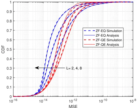
Fig. 1. The cumulative distribution of the channel estimation MSEǫq
mkfor
the schemes estimate-and-quantize (EQ) in (27) and quantize-and-estimate (QE) in (32) withK= 20,M= 200and Transmit Power= 0dBW
In Fig 1, we first validate with simulations our analytical MSE approximations which are obtained in (27) and (32) using Bussgang decomposition. Note that in our simulation setup the large scale fading has very small value up to -17 order of magnitude. This boils down to very small channel gain and to very small typical value of MSE. It is shown in Fig. 1 that our analyses for both strategies are quite close to simulations especially for small L and high transmit power. In at least
Using the corresponding channel estimation errors we then evaluate the average achievable rates per user given in (44). In this case, we compare their performance in terms of their per-user net throughput defined as
Su,kZF ,B
1−τp/τc
2 R
ZF
u,k, (46)
where the CSI overhead is taken into account by the term
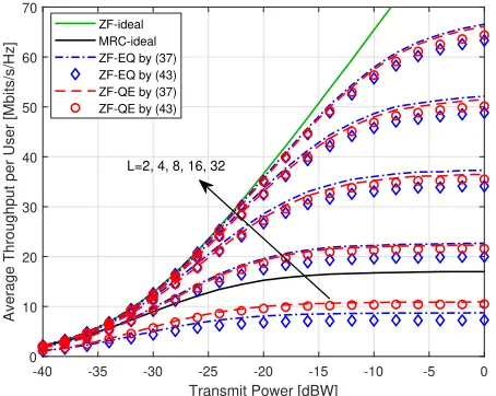
1 −τp/τc. As shown in Fig. 2 the QE scheme achieves higher throughput than the EQ scheme for small L over the whole range of transmit power. The performance gap is decreasing as we increase the quantization level. For small
L, the achievable rates computed by our approximation (43) has only relatively small deviation from the rate computed by (37). It can also clearly be observed that ZF with low quantization level L = 4 can already outperform MRC even with infinite quantization precision. This demonstrates the great improvement resulting from having global CSI available at the CPU. With L = 32 = 5-bits we are about 5 dB away from ZF with ideal fronthaul to reach 60Mbits/s/Hz average throughput per user. Meanwhile, the trade off between the increasing throughput and the resulting latency due to CSI overhead is left for future works.
-40 -35 -30 -25 -20 -15 -10 -5 0
Transmit Power [dBW] 0
10 20 30 40 50 60 70
Average Throughput per User [Mbits/s/Hz]
ZF-ideal MRC-ideal ZF-EQ by (37) ZF-EQ by (43) ZF-QE by (37) ZF-QE by (43)
[image:6.612.61.288.326.507.2]L=2, 4, 8, 16, 32
Fig. 2. The average per user throughput for different number of quantization levelL, transmit power and CSI acquisition schemes forK= 20andM= 200.
VI. CONCLUSION
This paper shows the benefit of having global CSI at the CPU for the uplink of cell-free massive MIMO. We have established the MSE expression of CSI-acquisition strategies and compared their performance. We have presented their corresponding average throughput for ZF detection. In this case, the low-complexity scheme ZF-QE outperforms ZF-EQ at low resolution especially for 1-bit.
APPENDIXA
DERIVATION OFEQUATION(31)AND(32)
For the estimator in (31) we havecqemkthat minimizes the MSE given by
cqemk=
Re{E{rq∗
p,mkgmk}} E{|rq
p,mk|2}
. (47)
From (29) we can express the numerator ofcqemk as
Re{E{rqp,mk∗ gmk}}=αqeRe{E{r∗p,mkgmk}}+Re{E{ϕHkdqegmk}}
=αqe√τpρpβmk, (48) where the second term vanishes due to uncorrelation. Likewise we can express the denominator as
E{|rq p,mk|
2
}=α2qeE{|rp,mk|2}+E{|ϕHk dqe|2}, (49) where the first term is given by
α2qeE{|rp,mk|2}=α2qe τpρp K
X
k′=1
βmk′|ϕHkϕk′|2+ 1
!
(50)
and the second term is given by
E{|ϕHkdqe|2}=kϕHkk2E{|dqe|2}
(13)
= (λqe−α2qe)E{|yp,m|2}
= (λqe−α2qe) ρp K
X
k=1
βmk+ 1
!
. (51) Letamk andbm denote the following expressions
amk,τpρp K
X
k′=1
βmk′|ϕHk ϕk′|2+ 1, andbm,ρp K
X
k=1
βmk+ 1, then we obtain
cqemk=αqe √τ
pρpβmk
αqeamk
αqeamk
α2
qeamk+ (λqe−α2qe)bm
=cmk
αqeamk
α2qeamk+ (λqe−α2qe)bm
. (52) Further, we have the MSE given by
ǫqemk=E{|gmk|2} −
(E{rqp,mk∗ gmk})2
E{|rqp,mk|2} , (53) where the second term can also be expressed as
γmkqe =α
2
qeτ ρpβ2mk
α2qeamk
α2qeamk
α2qeamk+ (λqe−α2qe)bm
=γmk
α2qeamk
α2
qeamk+ (λqe−α2qe)bm
. (54)
REFERENCES
[1] H. Q. Ngo, A. Ashikhmin, H. Yang, E. G. Larsson, and T. L. Marzetta, “Cell-Free Massive MIMO Versus Small Cells,”IEEE Transactions on Wireless Communications, vol. 16, no. 3, pp. 1834–1850, March 2017. [2] T. L. Marzetta, “Noncooperative Cellular Wireless with Unlimited
Num-bers of Base Station Antennas,”IEEE Transactions on Wireless Commu-nications, vol. 9, no. 11, pp. 3590–3600, Nov. 2010.
[3] E. Nayebi, A. Ashikhmin, T. L. Marzetta, H. Yang, and B. D. Rao, “Pre-coding and Power Optimization in Cell-Free Massive MIMO Systems,”
IEEE Transactions on Wireless Communications, vol. 16, no. 7, pp. 4445– 4459, July 2017.
[4] R. Irmer, H. Droste, P. Marsch, M. Grieger, G. Fettweis, S. Brueck, H. Mayer, L. Thiele, and V. Jungnickel, “Coordinated multipoint: Con-cepts, performance, and field trial results,”IEEE Communications Mag-azine, vol. 49, no. 2, pp. 102–111, February 2011.
[5] J. Bussgang, “Crosscorrelation functions of amplitude-distorted gaussian signals,”RLE Technical Reports, vol. 216, 1952.
[6] P. Zillmann, “Relationship Between Two Distortion Measures for Mem-oryless Nonlinear Systems,” IEEE Signal Processing Letters, vol. 17, no. 11, pp. 917–920, Nov. 2010.
[7] A. Burr, M. Bashar, and D. Maryopi, “Cooperative Access Networks: Optimum Fronthaul Quantization in Distributed Massive MIMO and Cloud RAN,” 2018 IEEE 87th Vehicular Technology Conference (VTC Spring), June 2018.
[8] B. Hassibi and B. M. Hochwald, “How Much Training is Needed in Multiple-Antenna Wireless Links?” IEEE Transactions on Information Theory, vol. 49, no. 4, pp. 951–963, April 2003.