Uniform Quantization
.
White Rose Research Online URL for this paper:
http://eprints.whiterose.ac.uk/148143/
Version: Accepted Version
Article:
Bashar, Manijeh, Cumanan, Kanapathippillai orcid.org/0000-0002-9735-7019, Burr, Alister
Graham orcid.org/0000-0001-6435-3962 et al. (3 more authors) (Accepted: 2019) Max-Min
Rate of Cell-Free Massive MIMO Uplink with Optimal Uniform Quantization. IEEE
Transactions on Communications. ISSN 0090-6778 (In Press)
[email protected] https://eprints.whiterose.ac.uk/
Reuse
Items deposited in White Rose Research Online are protected by copyright, with all rights reserved unless indicated otherwise. They may be downloaded and/or printed for private study, or other acts as permitted by national copyright laws. The publisher or other rights holders may allow further reproduction and re-use of the full text version. This is indicated by the licence information on the White Rose Research Online record for the item.
Takedown
If you consider content in White Rose Research Online to be in breach of UK law, please notify us by
Max-Min Rate of Cell-Free Massive MIMO Uplink
with Optimal Uniform Quantization
Manijeh Bashar,
Student Member, IEEE, Kanapathippillai Cumanan,
Member, IEEE, Alister G. Burr,
Senior
Member, IEEE, Hien Quoc Ngo,
Member, IEEE, Merouane Debbah,
Fellow, IEEE, and Pei Xiao,
Senior
Member, IEEE
Abstract—Cell-free Massive multiple-input multiple-output (MIMO) is considered, where distributed access points (APs) multiply the received signal by the conjugate of the estimated channel, and send back a quantized version of this weighted signal to a central processing unit (CPU). For the first time, we present a performance comparison between the case of perfect fronthaul links, the case when the quantized version of the estimated channel and the quantized signal are available at the CPU, and the case when only the quantized weighted signal is available at the CPU. The Bussgang decomposition is used to model the effect of quantization. The max-min problem is studied, where the minimum rate is maximized with the power and fronthaul capacity constraints. To deal with the non-convex problem, the original problem is decomposed into two sub-problems (referred to as receiver filter design and power allocation). Geometric programming (GP) is exploited to solve the power allocation problem whereas a generalized eigenvalue problem is solved to design the receiver filter. An iterative scheme is developed and the optimality of the proposed algorithm is proved through uplink-downlink duality. A user assignment algorithm is proposed which significantly improves the performance. Numerical results demonstrate the superiority of the proposed schemes.
Keywords: Cell-free Massive MIMO, generalized eigenvalue, ge-ometric programming, limited fronthaul.
I. INTRODUCTION
Cell-free Massive multiple-input multiple-output (MIMO) has been recognized as a potential technology for 5th Gener-ation (5G) systems, where large number of distributed access points (APs) serve a much smaller number of users, and hence, uniformly good service performance for all users is
M. Bashar, K. Cumanan and A. G. Burr are with the Department of Electronic Engineering, University of York, Heslington, York, U.K. e-mail: {mb1465, kanapathippillai.cumanan, alister.burr}@york.ac.uk. M. Bashar is also with home of the 5G Innovation Centre, Institute for Communica-tion Systems, University of Surrey, U.K. e-mail: [email protected]. H. Q. Ngo is with the School of Electronics, Electrical Engineering and Computer Science, Queen’s University Belfast, Belfast, U.K. e-mail: [email protected]. M. Debbah is with the Large Networks and Systems Group (LANEAS), CentraleSupelec, Universite Paris-Saclay, Gif-sur-Yvette 91192, France, and also with the Mathematical and Algorithmic Sciences Lab, Huawei Technologies Co., Ltd., Boulogne-Billancourt 92100, France. e-mail: [email protected]. Pei Xiao is with home of the 5G Innovation Centre, Institute for Communication Systems, University of Surrey, U.K. e-mail: [email protected].
The work of K. Cumanan and A. G. Burr was supported by H2020-MSCA-RISE-2015 under grant number 690750.
The work of H. Q. Ngo was supported by the UK Research and Innovation Future Leaders Fellowships under Grant MR/S017666/1.
The work of P. Xiao was supported in part by the European Commission under the 5GPPP project 5GXcast (H2020-ICT-2016-2 call, grant number 761498) as well as by the U.K. Engineering and Physical Sciences Research Council under Grant EP/ R001588/1.
ensured [1]–[5]. Interestingly, in [2], it is shown that the system performance of cell-free Massive MIMO depends only on large-scale fading, i.e., the small-scale fading and noise can be averaged out when number of APs is large. In [6] a user-centric approach is proposed where each user is served by a small number of APs. Cell-free Massive MIMO effectively implements a user-centric approach [7]. In [8], the authors consider distributed Massive MIMO in a multi-cell manner, which is different from cell-free massive MIMO (as there is no cell concept).
One of the main issues of cell-free Massive MIMO sys-tems which requires more investigation is the limited-capacity fronthaul links from the APs to a central processing unit (CPU). The assumption of infinite fronthaul in [1], [2], [9] is not realistic in practice. The fronthaul requirements for Massive MIMO systems, including small-cell and macro-cell base stations (BSs) have been investigated in [10]. The fronthaul load is the main challenge in any distributed antenna systems [10], [11]. First, we consider the case where all APs send back the quantized version of the minimum mean-square error (MMSE) estimate of the channel from each user and the quantized version of the received signal to the CPU. We next study the case when each AP multiplies the received signal by the conjugate of the estimated channel from each user, and sends back a quantized version of this weighted signal to the CPU. We derive the total number of bits for both cases and show that given the same fronthaul capacity for both cases, the relative performance of the aforementioned cases depends on the number of antennas at each AP, the total number of APs and the channel coherence time. A new approach is provided to the analysis of the effect of fronthaul quantization on the uplink of cell-free Massive MIMO. While there has been significant work in the context of network MIMO on compression techniques such as Wyner-Ziv coding for interconnection of distributed base stations, here for simplicity (and hence improved scalability) we assume simple uniform quantization. We exploit the Bussgang decomposition [12] to model the effect of quantization.
from the linear receiver at the APs. The proposed receiver filter provides more freedom in the design parameters and hence, significantly improves the performance of the uplink of cell-free Massive MIMO. The work in [14] presents a large scale fading decoding (LSFD) postcoding vector and power allocation scheme to solve max-min signal-to-interference-plus-noise ratio (SINR) problem. However, note that the work in [14] does not present any iterative algorithm to jointly solve power minimization problem and LSFD postcoding vector design. In [15], the authors use a bisection search approach to solve the power allocation problem. Next, MMSE receiver is exploited to determine the LSFD postcoding vectors. However, in our work, we exploit geometric programming (GP) to optimally solve the power allocation problem. Moreover, we prove that the proposed algorithm is optimal whereas the authors in [14] does not present any proof of optimality. In addition, the work in [14] does not consider any quantization errors whereas our work investigates the realistic assumption of limited-capacity fronthaul links.
We next investigate an uplink max-min rate problem with limited fronthaul links. In particular, the receiver filter coef-ficients and power allocation are optimized in the proposed scheme whereas the work in [2] only considered user power allocations. In particular, we propose a new approach to solve this max-min problem. A similar max–min rate problem based on SINR known as SINR balancing in the literature has been considered [16]–[23]. In [24], [25], the authors consider MIMO systems and study the problem of max-min user rate to maximize the smallest user rate. The problem of uplink-downlink duality has been investigated in [26], [27]. Note that none of the previous works on uplink-downlink duality consider Massive MIMO and the SINR formula in single-cell does not include any pilot contamination, channel estimation and quantization errors. To tackle the non-convexity of the original max-min rate problem, we propose to decouple the original problem into two sub-problems, namely, receiver filter coefficient design, and power allocation. We next show that the receiver filter coefficient design problem may be solved through a generalized eigenvalue problem [28]. Moreover, the user power allocation problem is solved through standard GP [29]. We present an iterative algorithm to alternately solve each sub-problem while one of the design parameters is fixed. Next an uplink-downlink duality for cell-free Massive MIMO system with limited fronthaul links is established to validate the optimality of the proposed scheme. We finally propose an efficient user assignment algorithm and show that further improvement is achieved by the proposed user assignment algorithm.
[image:3.612.329.543.52.209.2]The idea of exploiting an iterative algorithm to design the receiver filter and power coefficients in cell-free Massive MIMO system has been proposed in [30]. However, in [30], the authors investigate a cell-free Massive MIMO with single-antenna APs and perfect fronthaul links whereas in the this work we exploit a cell-free Massive MIMO system with multiple-antenna APs and limited-capacity fronthaul links. Furthermore, in this work, unlike [30], user assignment is investigated. The contributions of the paper are summarized as follows:
Figure 1. The uplink of a cell-free Massive MIMO system withK single-antenna users andMAPs. Each AP is equipped withN antennas. The solid lines denote the uplink channels and the dashed lines present the limited-capacity fronthaul links from the APs to the CPU.
1. We consider two cases: i) the quantized versions of the channel estimates and the received signals at the APs are available at the CPU and ii) the quantized versions of processed signals at the APs are available at the CPU. The corresponding achievable rates are derived by using the Use-and-then-Forget (UaF) bounding technique taking into account the effects of channel estimation error and quantization error.
2. We make use of the Bussgang decomposition to model the effect of quantization and present the analytical solution to find the optimal step size of the quantizer.
3. We propose a max-min fairness power control problem which maximizes the smallest of all user rates under the per-user power and fronthaul capacity constraints. To solve this problem, the original problem is decomposed into two sub-problems and an iterative algorithm is devel-oped. The optimality of the proposed algorithm is proved through establishing the uplink-downlink duality for the cell-free Massive MIMO system with limited fronthaul link capacities.
4. A novel and efficient user assignment algorithm based on the capacity of fronthaul links is proposed which results in significant performance improvement.
The rest of the paper is organized as follows. Section II de-scribes the system model and Section III provides performance analysis. The proposed max-min rate scheme is presented in Section IV and the convergence is provided in Section V. The optimality of the proposed scheme is proved in Section VI. Section VII investigates the proposed user assignment algorithm. Numerical results are presented in Section VIII, and finally Section IX concludes the paper.
II. SYSTEM MODEL
We consider uplink transmission in a cell-free Massive MIMO system with M APs and K single-antenna users ran-domly distributed in a large area. Moreover, we assume each AP has N antennas. The channel coefficient vector between the kth user and the mth AP, gmk ∈ CN×1, is modeled as gmk =√βmkhmk, where βmk denotes the large-scale fading,
(i.i.d.) CN(0,1) random variables, and represents the small-scale fading [2].
A. Uplink Channel Estimation
All pilot sequences transmitted by theKusers in the channel estimation phase are collected in a matrixΦ∈Cτp×K, where
τp is the length of the pilot sequence for each user and the
kth column,φφφk, represents the pilot sequence used for thekth
user. After performing a de-spreading operation, the MMSE estimate of the channel coefficient between the kth user and the mth AP is given by [2]
ˆ
gmk=cmk √τpppgmk+√τppp K
Õ
k′,k
gmk′φφφkH′φφφk+Wp,mφφφk
!
, (1)
where Wp,m ∈ CM×K denotes the noise sequence at the
mth AP whose elements are i.i.d.CN(0,1), pp represents the
normalized SNR of each pilot sequence (which we define in Section VIII), andcmk=
√τpppβmk
τpppÍKk′=1βmk′|φφφkH′φφφk|2+1
.Note that, as
in [2], we assume that the large-scale fading, βmk, is known.1
The investigation of cell-free Massive MIMO with realistic COST channel model [33]–[35] will be considered in our future work.
B. Optimal Quantization Model
Based on Bussgang’s theorem [12], a nonlinear output of a quantizer can be represented as a linear function as follows:
Q(z)=h(z)=az+nd, ∀k, (2)
where a is a constant value and nd refers to the distortion
noise which is uncorrelated with the input of the quantizer, z. The term a is given by
a= E{zh(z)}
E{z2} = 1
pz
∫
Z
zh(z)fz(z)d z, (3)
where pz =E{|z|2}
=E{z2} is the power of z and we drop absolute value aszis a real number, and fz(z)is the probability
distribution function of z. Denote by2
b=
Eh2(z)
E{z2} = 1
pz
∫
Z
h2(z)fz(z)d z. (4)
Then, the signal-to-distortion noise ratio (SDNR) is
SDNR=
E(az)2
E{n2
d}
= pza
2
pz b−a2
= a
2
b−a2, (5)
According to [12], [36], [37], the midrise uniform quantizer function h(z)is given by
h(z)=
−L−1
2 ∆ z≤ −
L
2 +1
∆,
l+12
∆ l∆≤z≤ (l+1)∆,l=−L2 +1,· · ·,L2 −2,
L−1
2 ∆ z≥
L
2 −1
∆,
(6)
1The large-scale fadingβ
mk changes very slowly with time. Compared to
the small-scale fading, the large-scale fading changes much more slowly, some 40 times slower according to [31], [32]. Therefore,βmkcan be estimated in
advance. One simple way is that the AP takes the average of the power level of the received signal over a long time period. A similar technique for collocated Massive MIMO is discussed in Section III-D of [32].
2Equations (2)-(4) come from [12] but we include them here for
complete-ness, and to define the terms we used.
where∆is the step size of the quantizer and L =2α, where α is number of quantization bits.
Lemma 1. The terms a and b are obtained as follows:
a=∆
s 2
πpz
© « L 2−1 Õ
l=1 e−
l2∆2 2pz +1ª®®®
¬
,b=∆ 2
pz©
« 1 4+4
L 2−1 Õ
l=1 lQ
l
∆
√p
z
ª® ¬
, (7)
where Q(x) is the Q-function and is given by Q(x) =
1
2erfc
x
√ 2
, where erfc refers to the complementary error function [38].
Proof:Please refer to Appendix A. In general, terms a and b are functions of the power of the quantizer input,pz. To remove this dependency, we normalize
the input signal by dividing the input signal, z, by the square root of its power,√pz, and then multiply the quantizer output
by its square root,√pz. Hence, by introducing a new variable
Û z=√zp
z, we have
Q(z)=√pzQ(Ûz)=aÛ√pzzÛ+√pznÛd=azÛ +√pznÛd. (8)
Note that (8) enables us to find the optimum step size of the quantizer and the corresponding a. Note that for the case ofÛ
Û
∆=√1p
z∆, we haveaÛ=a,bÛ=b. The optimal step size of the
quantizer is obtained by solving the following maximization problem:
∆opt=arg max
∆
SDNR=arg max
∆
a2 b−a2
I1
=arg max
Û
∆
Û a2 Û b− Ûa2
=arg max Û
∆
Û a2
Û b
I2
,arg max Û
∆
© «
2∆Û2 π
ÍL
2−1
l=1 exp
−l2∆Û2 2
+1
2
Û
∆21
4 +4
ÍL 2−1
l=1 lQ l∆Û ª®®®
¬
=arg max
Û
∆
© «
ÍL
2−1
l=1 2 exp
−l 2∆Û2
2
+1
2
1
4+4
ÍL 2−1
l=1 l Q l∆Û
ª® ®® ®® ¬
, (9)
where in step I1, we have used (8) and step I2 comes from results in Lemma 1. Moreover, note that ∆Û = √∆p
z. The
maximization problem in (9) can be solved through a one-dimensional search over ∆Û for a given L in a symbolic mathematics tool such as Mathematica. For the input zÛ with pzÛ =1, the optimal step size of the quantizer∆Ûopt, the resulting
distortion noise power, pnÛd = E{| Ûnd|
2}
= bÛ − Ûa2, and the resulting aÛ are summarized in Table I.
Remark 1. Interestingly, the optimal values for quantization
Table I
THE OPTIMAL STEP SIZE AND DISTORTION POWER OF A UNIFORM QUANTIZER WITHBUSSGANG DECOMPOSITION.
α ∆Ûopt σe2Û=pnÛd=bÛ− Ûa
2 aÛ
1 1.596 0.2313 0.6366 2 0.9957 0.10472 0.88115 3 0.586 0.036037 0.96256 4 0.3352 0.011409 0.98845 5 0.1881 0.003482 0.996505 6 0.1041 0.0010389 0.99896 7 0.0568 0.0003042 0.99969 8 0.0307 0.0000876 0.999912
C. Uplink Transmission
In this subsection, we consider the uplink data transmission, where all users send their signals to the APs. The transmitted signal from thekth user is represented byxk =√ρqksk,where
sk (E{|sk|2}=1) and qk denotes the transmitted symbol and
the transmit power from the kth user, respectively, where ρ represents the normalized uplink SNR (see Section VIII for more details). The N×1 received signal at the mth AP from all users is given by
ym=√ρ K
Õ
k=1
gmk√qksk+nm, (10)
where each element of nm ∈ CN×1, nn,m ∼ CN(0,1) is the
noise at the mth AP.
III. PERFORMANCEANALYSIS
In this section, the performance analysis for two cases is presented. First we consider the case when the quantized versions of the channel estimates and the received signals are available at the CPU. Next, it is assumed that only the quantized versions of the weighted signals are available at the CPU. The corresponding achievable rates are derived by exploiting the UaF bounding technique.
Case 1. Quantized Estimate of the Channel and Quantized
Signal Available at the CPU: Themth AP quantizes the terms
ˆ
gmk, ∀k, and ym, and forwards the quantized channel state
information (CSI) and the quantized signals in each symbol duration to the CPU. The quantized signal can be obtained as:
Q ([ym]n)=aÛ[ym]n+[eym]n=[ζm]n+j[νm]n, ∀m,n, (11)
where [eym]n refers to the quantization error, and [ζm]n and
[νm]n are the real and imaginary parts of the output of the
quantizer, respectively. Note that we separately quantize the imaginary and real parts of the input of the quantizer. Note that [x]n represents the nth element of vector x. The
analog-to-digital converter (ADC) quantizes the real and imaginary parts of[ym]n withαbits each, which introduces quantization errors[eym]nto the received signals [40], [41]. In addition, the
ADC quantizes the MMSE estimate of CSI as:
Q ([gˆmk]n)=aÛ[gˆmk]n+[emkg ]n =[̺mk]n+j[κmk]n,∀k,n, (12)
where [̺mk]n and [κmk]n denote the real and imaginary
parts of the output of the quantizer, respectively. Again, note that the real and imaginary parts of the input of the quantizer are separately quantized. For simplicity, we
assume all APs use the same number of bits to quan-tize the received signal, ym, and the estimated channel,
ˆ
gmk. Therefore, [eym]n = E{|[ym]n|2}[Ûeym]n and [egmk]n =
E{|[gˆmk]n|2}[Ûeg
mk]n, where En[Ûe y m]n
2o
=En[Ûegmk]n
2o
=σe2Û. Note thatEn[Ûey
m]n
2o
andEn[Ûeg mk]n
2o
are quantization errors
of a quantizer with normalized input[Ûym]n=√ [ym]n
E{ |[ym]n|2}
and
[Ûgˆmk]n = √ [gˆmk]n
E{ |[gˆmk]n|2}
, respectively. Note that due to power
normalization, a,Û b, and optimal step size for (11) and (12)Û are the same and provided in Table I. The received signal for thekth user after using the maximum ratio combining (MRC) detector at the CPU is given by
rk=
M
Õ
m=1
umk(Q (gˆmk))HQ (ym)=
M
Õ
m=1 umk
Û
agˆmk+egmkˆ
H
Û aym+eym
=
M
Õ
m=1 umk
Û
agˆmk+egmkˆ
H
Û a√ρ
K
Õ
k=1
gmk√qksk+aÛnm+eym
!
=aÛ2√ρE (ÕM
m=1
umkgˆHmkgmk√qk
)
| {z }
DSk
sk+aÛ2
M
Õ
m=1
umkgˆHmknm
| {z }
TNk
+aÛ2√ρ
M
Õ
m=1
umkgˆHmkgmk√qk−E
(ÕM
m=1
umkgˆHmkgmk√qk
)!
| {z }
BUk
sk+aÛ2
K
Õ
k′,k
√ ρ
M
Õ
m=1
umkgˆmkH gmk′√qk′ | {z }
IUIk k′
sk′+ K
Õ
k′=1 Û a√ρ
M
Õ
m=1
umk(egmkˆ )Hgmk′√qk′ | {z }
TQEk k′
sk′
+aÛ
M
Õ
m=1
umk(egmk)Hnm
| {z }
TQEgk
+aÛ
M
Õ
m=1
umkgˆHmke y m
| {z }
TQEyk
+
M
Õ
m=1 umk
egˆ
mk
H eym | {z }
TQEg yk
,(13)
where DSk and BUk denote the desired signal (DS) and
beamforming uncertainty (BU) for the kth user, respectively, and IUIk represents the inter-user-interference (IUI) caused by
thek′th user. In addition, TNkaccounts for the total noise (TN)
following the MRC detection, and finally the terms TQEyk, TQEgk, TQEgyk and TQEkk′ refer to the total quantization
error (TQE) at the kth user due to the quantization errors at the channel and signal. Moreover, by collecting all the coefficientsumk,∀m, corresponding to the kth user, we define uk = [u1k,u2k,· · ·,uM k]T and without loss of generality, it
is assumed that ||uk|| = 1. The optimal values of umk are
investigated in Section IV.
Proposition 1. Terms DSk, BUk, IUIkk′, TQNkk′, TQNgk,
TQNyk, TQNgyk are mutually uncorrelated.
Proof:Please refer to Appendix B.
SINRCase 1k = aÛ
4 |DSk|2
Û
a4En|BUk|2o+aÛ4En|TNk|2o+aÛ4ÍKk′,kEn|IUIkk′|2
o
+aÛ2E
TQEy
k
2
+aÛ2E
TQEg
k
2
+aÛ2
K
Í
k′=1
En|TQEkk′|2
o
+E
TQEgy
k
2.(14)
SINRCase 1k =
N2qkÍmM
=1umkγmk
2
N2ÍK
k′,kqk′ÍMm=1umkγmk
βmk′
βmk
2 φφφH
k φφφk′
2
+N
Ctot
Û a4 +1
ÍM
m=1umkγmkÍKk′=1qk′βmk′+N
ρ
Ctot
Û a4 +1
ÍM
m=1umkγmk
.(15)
systems. The tightness of this bound for cell-free Massive MIMO is presented in [2]. Using Proposition 1 and the UaF bounding technique in [2], we can obtain an achievable rate
as RCase 1k = log2(1+SINRCase 1k ), where SINR
Case 1
k is given
by (14). The closed-form expression for the achievable uplink rate of thekth user is given in the following theorem.
Theorem 1. Having the quantized CSI and the quantized
signal at the CPU and employing MRC detection at the CPU, the closed-form expression for the achievable rate of the kth user is given by RCase 1
k = log2(1+SINRCase 1k ), where the
SINRCase 1k is given by (15) (defined at the top of this page),
where γmk=√τpppβmkcmk and Ctot=2aÛ2σe2Û+σe4Û.
Proof: The power of quantization errors can be obtained as
En[ey m]n
2o
=En[Ûeym]n
2o
ρ
K
Õ
k′=1
qk′βmk′+1 !
,
En[eg mk]n
2o
=En[Ûegmk]n
2o
γmk. (16)
Since En[Ûeym]n2o =En[Ûeg mk]n
2o
=σe2Û, we have:
En[ey m]n
2o
=σe2Û ρ K
Õ
k′=1
qk′βmk′+1 !
,
En[eg mk]n
2o
=σe2Ûγmk. (17)
Using (16) and the fact that quantization error is indepnedent with the input of the quantizer, after some mathematical manipulations, we have:
Û
a2EnTQEy k
2o
+aÛ2EnTQEgk
2o
+aÛ2
K
Õ
k′=1
E|TQE kk′|2
+EnTQEgy k
2o
=NCtot
M
Õ
m=1
umkγmk ρ K
Õ
k′=1
qk′βmk′+1
!
.(18)
Note that the terms |DSk|2, E|BUk|2 , and E|IUIkk′|2 are
derived in (50), (51) and (56), respectively. Finally substituting (18), (50), (51) and (56) into (14) results in (15), which
com-pletes the proof of Theorem 1.
Case 2. Quantized Weighted Signal Available at the CPU:
The mth AP quantizes the terms zm,k = gˆmkH ym, ∀k, and
forwards the quantized signals in each symbol duration to the CPU as
zmk =gˆHmkym=rmk+j smk, ∀k,m, (19)
wherermk andsmk represent the real and imaginary parts of
zmk, respectively. An ADC quantizes the real and imaginary
parts of zm,k withαbits each, which introduces quantization
errors to the received signals [40]. Let us consider the term ezmk as the quantization error of the mth AP. Hence, using the Bussgang decomposition, the relation betweenzmkand its
quantized version, zÛmk, can be written as
Q (zmk)=azÛ mk+ezmk. (20)
Note that given the fact that the input of quantizer, i.e., zmk = gˆHmkym, is the summation of many terms, it can be
approximated as a Gaussian random variable. This enables us to exploit the values given in Table I, which are obtained for Gaussian input. The aggregated received signal at the CPU can be written as3
rk=
M
Õ
m=1
umkaÛgˆHmkym
|{z}
zmk
+ezmk
!
=aÛ√ρ
K
Õ
k′=1
M
Õ
m=1
umkgˆmkHgmk′√qk′sk′
+aÛ
M
Õ
m=1
umkgˆHmknm+
M
Õ
m=1
umkemkz =aÛ√ρE (ÕM
m=1
umkgˆHmkgmk√qk
)
| {z }
DSk
sk
+aÛ√ρ
M
Õ
m=1
umkgˆHmkgmk√qk−E
(ÕM
m=1
umkgˆHmkgmk√qk
)!
| {z }
BUk
sk+
K
Õ
k′,k
Û a
√ ρ
M
Õ
m=1
umkgˆHmkgmk′√qk′ | {z }
IUIk k′
sk′+aÛ M
Õ
m=1
umkgˆHmknm
| {z }
TNk
+
M
Õ
m=1 umkezmk
| {z }
TQEk
, (21)
where TQEk refers to the total quantization error (TQE) at the
kth user. Note that in cell-free Massive MIMO with M → ∞, due to the channel hardening property, detection using only the channel statistics is nearly optimal. This is shown in [2] (see Fig. 2 of reference [2] and its discussion). Moreover, in [2] the authors show that in cell-free Massive MIMO with M → ∞, the received signal includes only the desired signal plus interference from the pilot sequence non-orthogonality. Finally, using the analysis in [2], the corresponding SINR of the received signal in (21) can be defined by considering the worst-case of the uncorrelated Gaussian noise is given by (22)
3Note that for both Case 1 and Case 2, the AP estimates the channel.
Therefore the total complexity is the same for Case 1 and Case 2. However, in Case 1 the CPU performsN2multiplication andM−1additions whereas
in Case 2 the APs establish N multiplications and the CPU performs N
SINRCase 2k = |DSk|
2
E|BUk|2 + K
Í
k′,k
E|IUIkk′|2 +E|TNk|2 + 1
Û a2E
|TQEk|2
. (22)
SINRCase 2k ≈
N2qkÍMm=1umkγmk
2
N2 ÍK
k′,k
qk′
MÍ
m=1 umkγmk
βmk′
βmk
2 φφφHkφφφk′
2
+N M
Í
m=1 umk σ
2 Û
e(2βmk−γmk)
Û
a2 +γmk !
K
Í
k′=1
qk′βmk′+N
ρ σe2Û
Û a2+1
!
M
Í
m=1 umkγmk
.(23)
(defined at the top of the next page). Based on the SINR definition in (22), the achievable uplink rate of thekth user is given in the following theorem.
Theorem 2. Having the quantized weighted signal at the CPU
and employing MRC detection at the CPU, the achievable uplink rate of the kth user in the cell-free Massive MIMO system is R =log2(1+SINRCase 2), where SINRCase 2 is given by (23) (defined at the top of this page).
Proof:Please refer to Appendix C.
A. Required Fronthaul Capacity
Letτf be the length of the uplink payload data transmission
for each coherence interval, i.e.,τf =τc−τp,whereτcdenotes
the number of samples for each coherence interval and τp
represents the length of pilot sequence. Defining the number of quantization bits as αm,i, fori=1,2, corresponding to Cases 1 and 2, and mrefers to the mth AP. For Case 1, the required number of bits for each AP during each coherence interval is
2αm,1× (N K+Nτf) whereas Case 2 requires2αm,2× (Kτf)
bits for each AP during each coherence interval. Hence, the total fronthaul capacity required between themth AP and the CPU for all schemes is defined as
Cm=
2 N K+Nτfαm,1 Tc
, Case 1,
2 Kτfαm,2 Tc
, Case 2,
(24)
whereTc(in sec.) refers to coherence time.4 In the following,
we present a comparison between two cases of uplink trans-mission. To make a fair comparison between Case 1 and Case 2, we use the same total number of fronthaul bits for both cases, that is 2(N K+Nτf)αm,1 =2(Kτf)αm,2.5
IV. PROPOSEDMAX-MINRATESCHEME
In this section, we formulate the max-min rate problem for Case 2 of uplink transmission in cell-free Massive MIMO system, where the minimum uplink rates of all users is max-imized while satisfying the transmit power constraint at each user and the fronthaul capacity constraint. Note that the same
4Exploiting the constraintC
m ≤Cfh, the largest number of quantization
level is equal toαm,1= $
TcCfh 2
N K+Nτf
%
andαm,2= j
TcCfh
2Kτf
k
.
5Future work is needed to investigate the performance analysis for different
numbers of quantization bits as well as the numbers of APs. This will be presented in [15].
approach can be used to investigate the max-min rate problem for Case 1. The achievable user SINR for the system model considered in the previous section is obtained by following a similar approach to that in [2]. Note that the main difference between the proposed approach and the scheme in [2] is the new set of receiver coefficients which are introduced at the CPU to improve the achievable user rates. The benefits of the proposed approach in terms of the achieved user uplink rate is demonstrated through numerical simulation results in Section V. In deriving the achievable rates of each user, it is assumed that the CPU exploits only the knowledge of channel statistics between the users and APs to detect data from the received signal in (21). Using the SINR given in (23), the achiev-able rate is obtained RUPk = log2(1+SINRCase 2k ). Defining uk =[u1k,u2k,· · ·,uM k]T, Γk =[γ1k, γ2k,· · ·, γM k]T, Υkk′= diaghβ1k′
σ2
Û e(2β1k−γ1k)
Û
a2 +γ1k
,· · ·, βM k′ σ2
Û
e(2βM k−γM k) Û
a2 +γM k i
,
Λkk′=
γ1kβ1k′
β1k
,γ2kβ2k′ β2k
,· · ·,γM kβM k′ βM k
T
and
Rk =diag
"
σe2Û Û a2 +1
!
γ1k,· · ·,
σe2Û Û a2 +1
!
γM k
#
, the achievable
uplink rate of thekth user is given by Next, the max-min rate problem can be formulated as follows:
P1: max
qk,uk,α2 min
k=1,···,K R
UP
k (26a)
subject to ||uk||=1,∀k, 0≤qk ≤p(maxk), ∀k, (26b)
Cm ≤Cfh, ∀m, (26c)
where p(maxk) and Cfh refer to the maximum transmit power available at userk and the capacity of fronthaul link between each AP and the CPU, respectively. Note that using (24),Cm
is given asCm = 2(KτTfc)αm,2,∀m. Throughout the rest of the
paper, the index m is dropped from αm,i, i = 1,2, as we
consider the same number of bits to quantize the signal at all APs. Problem P1 is a discrete optimization with integer decision variables and it is obvious that the achievable user rates monotonically increase with the capacity of the fronthaul link between the mth AP and the CPU. Hence, the optimal solution is achieved whenCm=Cfh,∀m, which leads to fixed values for the number of quantization bits. As a result, the max-min based max-min rate problem can be re-formulated as follows:
P2: max
qk,uk
min
k=1,···,K R
UP
k (27a)
subject to ||uk||=1, ∀k, (27b)
Problem P2 is not jointly convex in terms of uk and power
allocation qk,∀k. Therefore, it cannot be directly solved
through existing convex optimization software. To tackle this non-convexity issue, we decouple Problem P2 into two sub-problems: receiver coefficient design (i.e. uk) and the power
allocation problem. The optimal solution for Problem P2, is obtained through alternately solving these sub-problems, as explained in the following subsections.
A. Receiver Filter Coefficient Design
In this subsection, the problem of designing the receiver coefficients is considered. We solve the max-min rate problem for a given set of allocated powers at all users,qk,∀k, and fixed
values for the number of quantization levels, Qm,∀m. These
coefficients (i.e.,uk,∀k) are obtained by independently
max-imizing the uplink SINR of each user. Therefore, the optimal receiver filter coefficients can be determined by solving the following optimization problem:
P3: max uk
(28a)
N2uH
k qkΓkΓ H k z
u
k
uHk
N2ÍK
k′,kqk′|φφφHkφφφk′|2Λkk′ΛHkk′+NÍKk′=1qk′Υkk′+NRk ρ
uk
subject to ||uk||=1, ∀k. (28b) Problem P3 is a generalized eigenvalue problem [28], [30], [44], where the optimal solutions can be obtained by de-termining the generalized eigenvector of the matrix pair
Ak = N2qkΓkΓkH and Bk = N2ÍKk′,kqk′|φφφkHφφφk′|2Λkk′ΛHkk′+
NÍKk′=1qk′Υkk′+NρRk corresponding to the maximum gener-alized eigenvalue.
B. Power Allocation
In this subsection, we solve the power allocation problem for a given set of fixed receiver filter coefficients, uk, ∀k,
and fixed values of quantization levels, Qm,∀m. The optimal
transmit power can be determined by solving the following max-min problem:
P4: max
qk
min
k=1,···,K SINR
UP
k (29a)
subject to 0≤qk ≤p(maxk) . (29b) Without loss of generality, Problem P4 can be rewritten by introducing a new slack variable as
P5: max
t,qk
t (30a)
subject to 0≤qk ≤p(maxk), ∀k,SINRUPk ≥t, ∀k. (30b)
Proposition 2. Problem P5can be formulated into a standard
GP.
Algorithm 1 Proposed algorithm to solve Problem P2
1.Initialize q(0)=[q(0)
1 ,q(
0) 2 ,· · ·,q(
0)
K ],i=1
2.Repeat steps 3-5 until SINR UP,(i)
k −SINR
UP,(i−1)
k
SINRUPk ,(i−1) ≤ ǫ,∀k
3. Determine the optimal receiver coefficients U(i) = [u(1i),u2(i),· · ·,u(Ki)]through solving the generalized eigenvalue ProblemP3 in (28) for a given q(i−1),
4.Computeq(i)through solving ProblemP5in (30) for a given
U(i)
5.i=i+1
Proof:Please refer to Appendix D. Therefore, Problem P5 is efficiently solved through exist-ing convex optimization software. Based on these two sub-problems, an iterative algorithm has been developed by al-ternately solving both sub-problems at each iteration. The proposed algorithm is summarized in Algorithm 1. Note that ǫ in Step 2 of Algorithm 1 refers to a small predetermined value.
V. CONVERGENCE
In this section, we present the convergence of the proposed Algorithm 1. We propose to alternatively solve two sub-problems to find the solution of the original ProblemP2, where at each iteration, one of the design parameters is determined by solving the corresponding sub-problem while other design variable is fixed. We showed that each sub-problem provides an optimal solution for the other given design variable. Let us assume at the i−1th iteration, that the receiver filter coefficientsu(i−1)
k ,∀kare obtained for a given power allocation q(i−1)and similarly, the power allocationq(i)is determined for a fixed set of receiver filter coefficientsu(i−1)
k ,∀k. Note that,
the optimal power allocationq(i)determined for a givenu(i−1)
k
achieves an uplink rate greater than or equal to that of the previous iteration. In addition, the power allocationq(i−1)is a feasible solution to find q(i) as the receiver filter coefficients
u(ki),∀k are determined for a givenq(i−1). Note that the uplink rate of the system monotonically increases with the power. As a result, the achievable uplink rate of the system monotonically increases at each iteration. Note that the achievable uplink max-min rate is bounded from above for a given set of per-user power constraints and fronthaul link capacity constraint. Hence the proposed algorithm converges to a specific solution. Note that to the best of our knowledge and referring to [1] this is a common way to show the convergence. In the next section, we prove the optimality of the proposed Algorithm 1 through the principle of uplink-downlink duality.
RUPk ≈log2 © «
1+
uH
k N
2q
kΓkΓkH
u
k
uHk
N2ÍK
k′,kqk′|φφφHkφφφk′|2Λkk′ΛHkk′+NÍKk′=1qk′Υkk′+N ρRk
uk
ª® ®® ® ¬
VI. OPTIMALITY OF THEPROPOSEDMAX-MINRATE ALGORITHM
In this section, we present a method to prove the optimality of the proposed Algorithm 1. The proof is based on two main observations: we first demonstrate that the original max-min Problem P2 with per-user power constraint is equivalent to an uplink problem with an equivalent total power constraint. We next prove that the same SINRs can be achieved in both the uplink and the virtual downlink with an equivalent total power constraint, which enables us to establish an uplink-downlink duality. Finally, we show that the virtual uplink-downlink problem is quasi-convex and can be optimally solved through a bisection search [45]. Note that the uplink Problem P1 and the equivalent virtual downlink problem achieve the same SINRs and the solution of the virtual downlink problem is optimal. As a result, the optimality of the proposed Algorithm 1 is guaranteed. The details of the proof are provided in the following subsections.
A. Equivalent Max-Min Uplink Problem
We aim to show the equivalence of Problem P2 with a per-user power constraint and the uplink max-min rate problem with a total power constraint. Note that in the total power constraint, the maximum available transmit power is defined as the sum of all users’ transmit power from the solution of Problem P2, which is formulated as:
P6 : max
qk,uk
min
k=1,···,K R
UP
k (31a)
subject to ||uk||=1, ∀k, (31b)
K
Õ
k=1
qk ≤Ptotc. (31c)
Problem P6 is not convex in terms of receiver filter coeffi-cients uk and power allocation qk,∀k. To deal with this
non-convexity, similar to the proposed method to solve problem P2, we propose to modify Algorithm 1 to incorporate the total power constraint in Problem P6. Hence, we decompose Problem P6 into receiver filter coefficient design and power allocation sub-problems. The same generalized eigenvalue problem in ProblemP3is solved to determine the receiver filter coefficients whereas the GP formulation in P5 is modified to incorporate the total power constraint (31c). Note that, the total power constraint is a convex constraint (posynomial function in terms of power allocation) and GP with the equivalent total power constraint can be used to find the optimum solution.
Lemma 2. The original Problem P2 (with per-user power
constraint) and the equivalent Problem P6(with the equivalent total power constraint) have the same optimal solution.
Proof: Please refer to Appendix E.
B. Uplink-Downlink Duality for Cell-free Massive MIMO
This subsection demonstrates an uplink-downlink duality for cell-free Massive MIMO systems. In particular, it is shown that the same SINRs (or rate regions) can be realized for all users in the uplink and the virtual downlink with the
equivalent total power constraints [27], [46], respectively. In other words, based on the principle of uplink-downlink duality, the same set of filter coefficients can be utilized in the uplink and the downlink to achieve the same SINRs for all users with different user power allocations. The following theorem defines the achievable virtual downlink rate for cell-free Massive MIMO systems:
Theorem 3. By employing conjugate beamforming at the APs,
the achievable virtual downlink rate of the kth user in the cell-free Massive MIMO system with K randomly distributed single-antenna users, M APs where each AP is equipped with N antennas and limited-capacity fronthaul links is given by (32) (defined at the top of this page).
Proof:This can be derived by following the same approach as for uplink transmission in Theorem 2. Note that in (32), pk, ∀k denotes the downlink
power allocation for the kth user and the following equalities hold: Γk = [γ1k, γ2k,· · ·, γM k]T, Fk′k = diaghβ1k
aÛ2(2β 1k′−γ1k′)
σ2
Û
e +
γ1k′
,· · ·, βM k
aÛ2(2β
M k′−γM k′)
σ2
Û
e +
γM k′ i
and ∆k′k =
γ1k′β1k
β1k′ ,
γ2k′β2k
β2k′ ,· · ·,
γM k′βM k
βM k′ T
. The
following Theorem provides the required condition to establish the uplink-downlink duality for cell-free Massive MIMO systems with limited-capacity fronthaul links:
Theorem 4. By employing MRC detection in the uplink and
conjugate beamforming in the virtual downlink, to realize the same SINR tuples in both the uplink and the virtual downlink of a cell-free Massive MIMO system, with the same fronthaul loads, the same filter coefficients and different transmit power allocations, the following condition should be satisfied:
N
M
Õ
m=1
K
Õ
k=1 σe2Û
Û a2 +1
!
γmk|wmk|2=
K
Õ
k=1
q∗k =Ptotc , (34)
where q∗
k, ∀k refer to the optimal solution of Algorithm 1, and
wmk denotes the(m,k)-th entry of matrixWwhich is defined
as follows:
W=[√p1u1,√p2u2,· · ·,√pKuK]. (35)
Proof:Please refer to Appendix F.
C. Equivalent Max-Min Downlink Problem
In this subsection, we provide an optimal solution for the max-min rate downlink problem with the equivalent total power constraint. This problem can be written as follows:
P7: max
pk,uk min
k=1,···,K R
DL
k (36a)
subject to ||uk||=1, ∀k,
K
Õ
k=1
pk ≤Ptotc, (36b)
whereRDLk =log2(1+SINRDLk ), and SINRDLk is defined in (32).
SINRDLk (U,p)= u H
k N
2p
kΓkΓHk uk
N2ÍK
k′,kuHk′pk′|φφφHk′φφφk|2∆k′k∆kH′kuk′+NÍKk′=1uHk′pk′Fk′kuk′+ Nρ
. (32)
SINRUPk (U,q)= u
H
k N
2q
kΓkΓkHuk uH
k
N2ÍK
k′,kqk′|φφφkHφφφk′|2Λkk′Λ H
kk′+NÍKk′=1qk′Υkk′+ N
ρRk
uk
.
(33)
it can be represented by introducing a new variable W to decouple the variables Uandqas follows:
P8: max
W k=min1,···,K R
DL
k (37a)
subject to N
M
Õ
m=1
K
Õ
k=1 σe2Û
Û a2 +1
!
γmk|wmk|2 ≤Ptotc. (37b)
It is easy to show that Problem P8 is quasi-convex. Hence, a bisection [45] approach can be used to obtain the optimal solution for the original Problem P8 by sequentially solving the following power minimization problem for a given target SINR t at all users:
P9: min W
M
Õ
m=1
K
Õ
k=1
γmk|wmk|2 (38a)
subject to (38b)
wHk N2ΓkΓkH
wk
N2ÍK
k′,kwHk′|φφφkH′φφφk|2∆k′k∆kH′kwk′+NÍKk′=1wkH′Fk′kwk′+Nρ
≥t,
N
M
Õ
m=1
K
Õ
k=1 σe2Û
Û a +1
!
γmk|wmk|2 ≤Ptotc, (38c)
wherewk represents thekth column of the matrixWdefined in
(35). Problem P9 can be reformulated by exploiting a second order cone programming (SOCP). Note that the objective function in (38) refers to the total transmit power. As a result, the optimal solution for Problem P7 can be obtained by extracting the normalized transmit filter coefficients uk’s
and power allocations pk’s as
p∗k =||w∗k||2, ∀k, & u∗k =
w∗ k
||w∗k||, ∀k, (39)
where the w∗k’s refer to the optimal solution of Problem P8. Note that constraint (38c) is an equivalent total power constraint to the per-user power constraint in the original Problem P2, which is a more relaxed constraint than (27c). However, it is already shown in the previous sub-section that the same SINRs can be realized in both the uplink and the virtual downlink with per-user and the equivalent total power constraints.
D. Prove of Optimality of Algorithm 1
In Lemma 2, we prove that Problems P2 and P6 are equivalent, and have the same solution. Next, in Proposition 1, using uplink-downlink duality, we prove that Problem P6 and the virtual downlink ProblemP7 are equivalent. Note that the SINR achieved by solving Problem P7 are optimal (the optimal solution is obtained by a bisection search approach).
This confirms that the proposed algorithm to solve Problem P2 is optimal.
VII. USERASSIGNMENT
Exploiting (24), it is obvious that the total fronthaul capacity required between the mth AP and the CPU increases linearly with the total number of users served by the mth AP. This motivates the need to pick a proper set of active users for each AP. Using (24), we have
α2×Km≤
CfhTc
2τf
, (40)
whereKmdenotes the size of the set of active users for themth
AP. From (40), it can be seen that decreasing the size of the set of active users allows for a larger number of quantization levels. Motivated by this fact, and to exploit the capacity of fronthaul links more efficiently, we investigate all possible combinations of α2 and Km. First, for a fixed value of α2, we find an upper bound on the size of the set of active users for each AP. In the next step, we propose for all APs that the users are sorted according to βmk,∀k, and find theKm users
which have the highest values ofβmkamong all users. If a user
is not selected by any AP, we propose to find the AP which has the best link to this user (in Algorithm 2, π(j)=argmax
m
βm j
determines best link to the jth user, i.e., the index of the AP which is closest to the jth user). Note that to only consider the users that have links to other APs, we use k|Skπj ,,
where refers to empty set. Then we drop the user which has the lowest βmk,∀k, among the set of active users for that
AP, which has links to other APs as well. Finally, we add the user which is not selected by any AP to the set of active users for this AP. We next solve the virtual downlink problem to maximize the minimum uplink rate of the users as follows
P10: max
W k=min1,···,K R
DL
k (®γmk), (41a)
subject to N
M
Õ
m=1
K
Õ
k=1 σe2Û
Û a2+1
!
®
γmk|wmk|2 ≤Ptotc, (41b)
where
® γmk=
γmk, m∈ Sk
0, otherwise (42)
whereSk refers to the set of active APs for thekth user. The
proposed algorithm is summarized in Algorithm 2.
VIII. NUMERICALRESULTS ANDDISCUSSION
Algorithm 2 User Assignment
1. Using (40), find the maximum possible integer value for Km,∀m
2. Sort users according to the ascending channel gain: βm1 ≥ βm2 ≥ · · · ≥ βmK,∀m
3.AssignKmusers with the highest values of βmk,∀mto each
AP, i.e., Tm← {k(1),k(2),· · ·,k(Km)},∀m
4. Find set of active APs for each user; Sk ←
{m(1),m(2),· · ·,m(Mk)},∀k
5. for j =1 :K
if size {Sj} =0 π(j)=argmax
m
βm j,δ(j)=argmin
k
βπ(j)k,k|Skπj ,,Tπ(j)←
Tπ(j)\δ(j),Tπ(j)← Tπ(j)∪j end
end
6. If m∈ Sk, thenγ®mk ←γmk, otherwiseγ®mk =0 and solve the max-min rate problem P2
D×Dsimulation area, where both APs and users are uniformly distributed at random. In the following subsections, we define the simulation parameters and then present the corresponding simulation results. The channel coefficients between users and APs are modeled in Section II where the coefficient βmk is
given by βmk=PLmk10 σs h zmk
10 ,where PL
mk is the path loss
from thekth user to themth AP and the second term10σs h zmk10 , denotes the shadow fading with standard deviation σsh = 8 dB, and zmk∼ N(0,1)[2]. In the simulation, an uncorrelated
shadowing model is considered and a three-slope model for the path loss similar to [2]. The noise power is given by pn = BW×kB ×T0 ×W, where BW = 20 MHz denotes the bandwidth, kB=1.381×10⁻²³ represents the Boltzmann constant, andT0 =290(Kelvin) denotes the noise temperature. Moreover, W = 9dB, and denotes the noise figure. It is assumed that that p¯pandρ¯denote the power of pilot sequence
and the uplink data powers, respectively, where pp =
¯
pp
pn
and ρ = pρ¯
n. In simulations, we set p¯p = 200 mW and ¯
ρ =200 mW. Similar to [2], we assume that the simulation area is wrapped around at the edges which can simulate an area without boundaries. Hence, the square simulation area has eight neighbours. We evaluate the average rate of the system over 300 random realizations of the locations of APs, users and shadow fading. Similar to the model in [47], the fronthaul links establish communications through wireless microwave links with limited capacity. Hence, we use Cfh=100Mbits/s [47], unless otherwise it is indicated. In this paper, the term “orthogonal pilots” refers to the case where unique orthogonal pilots are assigned to all users, while in “random pilot assignment” each user is randomly assigned a pilot sequence from a set ofτp orthogonal sequences of length
τp (<K), following the approach of [2].
1) Performance of Different Cases of Uplink Transmission: Fig. 2a presents the average per-user uplink rate, where the per-user uplink rate is obtained by solving Problem P4, given by (29) for Cases 1 and 2. The values of α1 =9 andα2 =2
correspond to a total number of 14,400 bits for each AP during each coherence time (or frame). In addition, similar to [40] we use a uniform quantizer with fixed step size. As Fig 2a shows the performance of Case 1 is slightly better than Case 2 for K=20. Next, the performance of the cell-free Massive MIMO system is evaluated for a system withK=40in which each AP is equipped withN=20antennas. Fig. 2a shows the average rate of the cell-free Massive MIMO system, where for Case 1 and Case 2, we set α1 = 3 and α2 = 8, respectively which leads to a total number of 64,000 fronthaul bits per AP per frame. Fig. 2a shows that the performances of Case 1 and Case 2 depend on the values of N, K and τf. Next,
we investigate the effect of number of antennas per AP and τf for K = 20. Fig. 2b shows the average per-user uplink
rate of cell-free Massive MIMO versus number of antennas per AP and two cases of τp = 20 (τf = 180) and τp = 10 (τf =190). Moreover, we consider (α1 =18, α2 =5), (α1 =
18, α2 = 10), (α1 = 18, α2 = 15) for the cases of N = 5, N = 10, N = 15, respectively, resulting 18,000 bits for all values ofN. As the figure shows the difference between Case 1 and Case 2 decreases asN increases. Moreover, for the case of orthogonal pilots and N = 15, the performance of Case 2 is better than the performance of Case 1. Since in case 1, the CPU knows the quantized channel estimates, other signal processing techniques (e.g., zero-forcing processing) can be implemented to improve the system performance and can be considered in future work.
2) Performance of the Proposed User Max-Min Rate Al-gorithm: In this subsection, we evaluate the performance of the proposed uplink max-min rate scheme. To assess the performance, a cell-free Massive MIMO system is considered with 70 APs (M = 70) where each AP is equipped with N =4 antennas and 40 users (K = 40) which are randomly distributed over the simulation area of size 1×1 km meters. Moreover, we consider the case {M = 50,N = 4,K = 30} Fig. 3 presents the cumulative distribution of the achievable uplink rates for the proposed Algorithm 1 in the case similar to [2], without defining the coefficientsuk, (i.e.,umk=1 ∀m,k)
and solving Problem P4, with random pilot sequences with length τp = 30. As seen in Fig. 3, the performance (i.e. the
10%-outage rate,Rout, refers to the case whenPout=Pr(Rk <
Rout)=0.1, where Pr refers to the probability function) of the proposed scheme is almost three times than that of the case withumk =1 ∀m,k.
3) Convergence: Next, we provide simulation results to validate the convergence of the proposed algorithm for a set of different random realizations of the locations of APs, users and shadow fading. These results are generated over the simulation area of size1×1km2with random and orthogonal pilot sequences. Fig. 4a investigates the convergence of the proposed Algorithm 1 with 70 APs (M = 70) and 40 users (K=40) and random pilot sequences with length τp = 30, whereas Fig. 4b demonstrates the convergence of the proposed Algorithm 1 for the case of M = 30 APs and K = 50
10 11 12 13 14 15 16
Number of APs (M)
0.5 1 1.5 2 2.5
Average per-user uplink rate (bits/s/Hz)
Case 1, K=20, N=4 Case 2, K=20, N=4 Case 1, K=40, N=20 Case 2, K=40, N=20
(a) Average per-user uplink rate for cases 1 and 2, with (N = 4,
K=20,τp=20,α1=9,α2=2), and (N=20,K=40,τp=40,
α1 =8, α2 =5) with D = 1km and τc = 200. Note that here
τf =τc−τp=160.
5 10 15
Number of antennas per AP (N) 1
1.5 2 2.5 3
Average per-user uplink rate (bis/s/Hz)
Case 1, p=20 Case 2, p=20 Case 1, p=10
Case 2, p=10
(b) Average per-user uplink rate for cases 1 and 2, forM=20,
K =20,τp =20,τp =10,D =1km andτc =200versus number of antennas per AP. Note that we consider(α1=18, α2=
5),(α1=18, α2=10),(α1=18, α2=15)for the cases ofN=5,
N=10,N=15, respectively. Figure 2. Performance of different cases of uplink transmission
0 0.5 1 1.5 2 2.5
Per-user uplink rate (bits/s/Hz) 0
0.1 0.2 0.3 0.4 0.5 0.6 0.7 0.8 0.9 1
Cumulative distribution
Proposed scheme (Algorithm 1)
u
mk=1 and solve
Problem P
4
M=70, N=4, K=40, =30
[image:12.612.88.513.69.234.2]M=30, N=8, K=50, =50
Figure 3. The cumulative distribution of the per-user uplink rate, for {M=
70,N=4,K=40},{M=50,N=4,K=30}, andτp=30,α1=1and
D=1km.
4) Uplink-Downlink Duality in Cell-Free Massive MIMO System: Here, the simulation results are provided to support the theoretical derivations of the uplink-downlink duality and the optimality of Algorithm 1. It is assumed that users are randomly distributed through the simulation area of size1×1
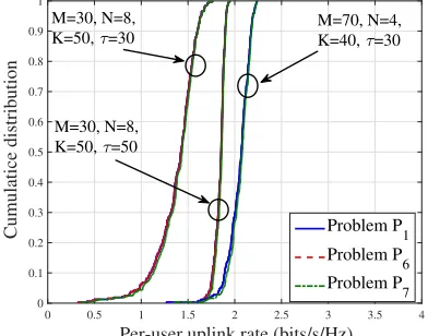
km. Figs. 5 compares the cumulative distribution of the achiev-able uplink rates between the original uplink max-min problem (Problem P1), the equivalent uplink problem (Problem P6) and the equivalent downlink problem (Problem P7). In Fig. 5, the minimum uplink rate is obtained for a system with 30 APs (M =30) where each is equipped with N =8 antennas and has 50 users (K =50) for two cases of orthogonal pilot sequences and random pilot sequences with length τp =30.
Moreover, Fig. 5 demonstrates the same results for 70 APs (M = 70), N = 4, 40 users (K = 40), and τp = 30. The
simulation results provided in Fig. 5 validate our result that the problem formulations P1, P6 and P7 are equivalent and
achieve the same minimum user rate. In addition, these results support our result on the uplink-downlink duality for cell-free Massive MIMO in Section VI and the proof of optimality of Algorithm 1.
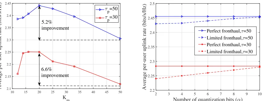
5) Performance of the Proposed User Assignment Algo-rithm 2: This subsection investigates the performance of the proposed user assignment Algorithm 2. In Fig. 6a, the average per-user uplink rate is presented with M = 120, N = 2, K = 50, orthogonal pilot sequences and random pilot assignment with D = 1 km, versus the total number of active users per AP. Here, we used inequality (40) and set α2×Km = 100 for all curves in Fig. 6a. The optimum value of Km, (Kmopt), depends on the system parameters and
as Fig. 6a shows for both cases of τp = 50 and τp = 30, the optimum value is achieved by Kmopt = 20. As a result, the proposed user assignment scheme can efficiently improve the performance of cell-free Massive MIMO systems with limited fronthaul capacity. For instance, using the proposed user assignment scheme for the case ofτp=50in Fig. 6a, one can achieve per-user uplink rate of2.442bits/s/Hz by setting Kmopt = 20, instead of quantizing the signals of all K = 40
users and achieving per-user uplink rate of 2.3 bits/s/Hz, which indicates more than 5.2% in the performance of cell-free Massive MIMO systems with limited fronthaul capacity.
6) Effect of the Capacity of Fronthaul Links: What is the optimal capacity of fronthaul links in cell-free Massive MIMO systems to approach the performance of the system with per-fect and error-free fronthaul links? The aim of this subsection is to answer this fundamental question. In this subsection, we evaluate the performance of the cell-free Massive MIMO system with two cases of perfect and limited fronthaul links. To assess the performance, a cell-free Massive MIMO system is considered with M = 120, K = 50, N = 2, D = 1 km, τp = 30 and τp = 50. To improve the performance of the
[image:12.612.63.270.307.483.2]