electrical impedance tomography
.
White Rose Research Online URL for this paper:
http://eprints.whiterose.ac.uk/144256/
Version: Accepted Version
Article:
Liu, D., Smyl, D. orcid.org/0000-0002-6730-5277 and Du, J. (2019) A parametric level
set-based approach to difference imaging in electrical impedance tomography. IEEE
Transactions on Medical Imaging, 38 (1). pp. 145-155. ISSN 0278-0062
https://doi.org/10.1109/TMI.2018.2857839
© 2018 IEEE. Personal use of this material is permitted. Permission from IEEE must be
obtained for all other users, including reprinting/ republishing this material for advertising or
promotional purposes, creating new collective works for resale or redistribution to servers
or lists, or reuse of any copyrighted components of this work in other works. Reproduced
in accordance with the publisher's self-archiving policy.
[email protected] https://eprints.whiterose.ac.uk/ Reuse
Items deposited in White Rose Research Online are protected by copyright, with all rights reserved unless indicated otherwise. They may be downloaded and/or printed for private study, or other acts as permitted by national copyright laws. The publisher or other rights holders may allow further reproduction and re-use of the full text version. This is indicated by the licence information on the White Rose Research Online record for the item.
Takedown
If you consider content in White Rose Research Online to be in breach of UK law, please notify us by
A Parametric Level Set based Approach to
Difference Imaging in Electrical Impedance
Tomography
Dong Liu
∗, Danny Smyl and Jiangfeng Du
∗Abstract—This paper presents a novel difference imaging approach based on the recently developed parametric level set (PLS) method for estimating the change in a target conductivity from electrical impedance tomography measurements. As in con-ventional difference imaging, the reconstruction of conductivity change is based on data sets measured from the surface of a body before and after the change. The key feature of the proposed approach is that the conductivity change to be reconstructed is assumed to be piecewise constant while the geometry of the anomaly is represented by a shape-based PLS function employing Gaussian radial basis functions (GRBF). The representation of the PLS function by using GRBF provides flexibility in describing a large class of shapes with fewer unknowns. This feature is advantageous, as it may significantly reduce the overall number of unknowns, improve the condition number of the inverse problem, and enhance the computational efficiency of the technique. To evaluate the proposed PLS-based difference imaging approach, results obtained via simulation, phantom study, and in vivo pig data are studied. We find that the proposed approach tolerates more modeling errors and leads to significant improvement in image quality compared with the conventional linear approach.
Index Terms—Electrical impedance tomography, parametric level set method, difference imaging, lung imaging, inverse problems.
I. INTRODUCTION
I
N medical electrical impedance tomography (EIT), harm-less electric currents are applied on a subject’s skin and the resulting voltages are measured with an electrode array attached on the body surface. From these boundary voltage measurements, it is possible to estimate the internal conduc-tivity distribution of the body. Medical applications include imaging of brain activity [1], monitoring of lung function [2]– [4], and detection of breast cancer [5] and thoracic vascular structures [6].Manuscript received January xx, 2018; revised xx, 2018; accepted xx. This work was supported in part by the National Key R&D Program of China (Grant No. 2018YFA0306600), in part by the NNSFC (Grants No. 81788101, No. 11227901 and No. 11761131011), in part by the CAS (Grants No. GJJSTD20170001 and No. QYZDY-SSW-SLH004), and in part by the Anhui Initiative in Quantum Information Technologies (Grant No. AHY050000) and Anhui Provincial Natural Science foundation under Grant 1708085MA25.
D. Liu and J. Du are with CAS Key Laboratory of Microscale Magnetic Resonance and Department of Modern Physics, University of Science and Technology of China (USTC), Hefei 230026, China, Hefei National Labo-ratory for Physical Sciences at the Microscale, USTC, China, and also with Synergetic Innovation Center of Quantum Information and Quantum Physics, USTC, China, e-mail: ([email protected], [email protected]).
D. Smyl is with Department of Mechanical Engineering, Aalto University, Espoo, Finland.
Asterisk indicates corresponding author.
One of the main challenges of EIT is that the image re-construction is a severely nonlinear ill-posed inverse problem; therefore, robust methods for handling noise and modeling errors and a stability-promoting regularization strategy are required. Methods for solving the EIT problem can generally be divided intoabsolute imaginganddifference imaging.
In absolute imaging, the aim is to estimate the absolute conductivity distribution based on measurements correspond-ing to a scorrespond-ingle state. The reconstruction of the absolute conductivity distribution requires accurate information of the auxiliary model parameters, i.e., electrode placement, size and shape, and the body shape or the domain boundary in general. Therefore, most of the algorithms assume that the electrode information and boundary of the body shape are exactly known
a priori, and the only unknown parameter is the conductivity distribution. In practice, knowledge of these auxiliary model parameters is incomplete and uncertain, especially in medical EIT applications. For example, in the thorax applications, the thorax shape varies due to breathing and changes of the patient position during the measurements. It has been shown that errors in these auxiliary model parameters, can lead to severe errors in the absolute reconstructions [7], [8].
On the other hand, in difference imaging, the variations in conductivity distributionw.r.tthe reference is estimated based on data sets collected before and after the conductivity change. For example, in lung imaging, the data before the change might be collected at respiratory inspiration and the data after the change at expiration, in such a way that the difference image shows the conductivity change between inspiration and expiration [2]–[4].
conductivity from EIT data and then inverting the transform. A detailed description of this method and its implementation is provided in, e.g. [20]. For difference applications discussing the utilities of the D-bar method, we refer the reader to [2], [21]–[23]. To this end, real-time capabilities of the D-bar method have also recently been demonstrated in [24]. It should be noted that, in the D-bar method, regularization is provided by low-pass filtering in the nonlinear frequency domain. However, the use of low-pass filtering of Fourier data commonly results in reconstructed images that may suffer from a loss of sharpness. 3 Linearization based methods, such as NOSER [25], back projection method [26] and GREIT [27], which are some of the most widely used methods. In the linearization based method, the relationship between the conductivity and measurement changes is often modeled by a linearized model, through a global linearization of the observation model. The linear difference reconstruction has been found to tolerate modeling errors caused by uncertainties in the auxiliary model parameters – to an extent. This feature occurs when the unknown auxiliary parameters are time-independent, leading to partial cancellation of the modeling errors when the difference of the measurements is computed [28].
Although the linear difference imaging approach is able to suppress some of the effects of modeling errors, previous studies have shown that artifacts are often present in the reconstructions [29], [30]. Furthermore, a drawback of the linear approach is that it is highly approximative since the actual forward mapping is inherently nonlinear in nature, such that it is only feasible for small deviations w.r.t the reference conductivity [31]. For example, in EIT imaging of lungs, significant accumulation of highly conductive liquids or low conducting air may violate the linear hypothesis, and thus the conventional linear approach may be inadequate for detecting clinically relevant information in the lung [32]. Moreover, the linearization point plays an important role in the performance of the linear approach [33]. A commonly used way of selecting the linearization point is to treat it as a homogeneous estimate of the conductivity of the initial state. However, in medical EIT, the initial state is often highly inhomogeneous. Consequently, modeling errors will be generated by a homogeneous approximation of the initial state. One such example is EIT lung imaging in which the low conducting lungs attract less current flow through the body center compared to that predicted by a uniform, homogeneous distribution [33]. Due to these problems, the conventional linear approach usually only provides qualitative information on the conductivity change.
Some exceptions to the above mentioned approaches exist: one approach is to reconstruct the background conductivity of the target simultaneously with the change of the conductivity based on EIT measurements before and after the change, via the inclusion of prior information in regularization terms for each state and the employment of compound regularization, see details in [7], [28]. Another approach is to compute absolute reconstructions of the conductivities before and after change based on the EIT measurements separately, and to obtain the reconstruction of conductivity change by subtracting
conductivity before change from conductivity after change. However, these two approaches belong to nonlinear iterative methods and the minimization of such problems is computa-tionally expensive. Therefore, from a practical point of view, they are not flexible approaches for real biomedical EIT.
Over the years, a wide variety of shape-based reconstruction methods have been proposed for many different applications. Among the shape-based reconstruction methods, the level set method (LSM) is likely the most common one [35]. Earlier relevant work in EIT includes the investigation of applying the level set method for locating the embedded objects, for examples see [36]–[39]. The key idea of LSM is to implicitly represent the conductivity distribution using a level set func-tion, and the interfaces between regions are represented as the zero level set. The conductivity reconstruction problem is then transformed into a shape reconstruction problem.
In this paper, we aim to alleviate the ill-posedness of the difference imaging reconstruction problem to some extent by incorporating some shape-prior information. Inspired from works [40], [41], here, we expand on our previous work in [42] where a parametric level set (PLS)-based approach was developed for absolute EIT. In this work, we consider the use of a shape-based approach to difference EIT based on a PLS formulation. In the proposed PLS-based difference imaging approach, we assume that the conductivity change to be reconstructed can be described as one or more embedded objects with unknown piecewise constant conductivity change values, and the geometry of the anomaly is represented by a PLS function employing Gaussian radial basis functions (GRBF). The representation of the PLS function by using GRBF provides flexibility in describing a large class of shapes with fewer unknowns. This brings at least the following advantages: 1 greatly reducing the overall number of un-knowns; 2 improving the condition number of the inverse problem; and 3 enhancing the computational efficiency of the technique. To solve the PLS-based inverse problem, an iterative regime aiming to improve the chance of reliably reconstructing conductivity change is employed.
Finally, we evaluate the performance of the proposed PLS-based difference imaging approach via simulation, phantom study, and in vivo pig data. Specifically, simulation data are used to show (i) PLS reconstructions for difference EIT in thorax imaging and (ii) the robustness of the PLS-based approach considering the width of the Gaussian radial basis function by varying the Gaussian width parameter. To study the robustness of the approachw.r.tgeometric modeling errors, we reconstruct images using both phantom and in vivo pig data. The results are compared against the conventional linear difference imaging approach.
II. FORWARD PROBLEM OFEIT
Let an imaged body under investigation occupy a two-or three- dimensional region Ω ⊂ Rq, q = 2,3, with its boundary denoted by ∂Ω. The forward problem of EIT can be stated as follows: given a conductivity distribution σ(x) within the domain of interestΩ, and a current injection pattern Iℓ, compute the electrical potential u(x) at the measuring
electrodes. In this study, the so-called complete electrode model (CEM) is employed [43]. Mathematically, the forward problem of the CEM is stated as follows:
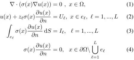
∇ ·(σ(x)∇u(x)) = 0, x∈Ω, (1) u(x) +zℓσ(x)
∂u(x)
∂n =Uℓ, x∈eℓ, ℓ= 1, ..., L (2) Z
eℓ
σ(x)∂u(x)
∂n dS =Iℓ, ℓ= 1, ..., L (3)
σ(x)∂u(x)
∂n = 0, x∈∂Ω\
L
[
ℓ=1
eℓ (4)
where x∈ Ωis the spatial coordinate, zℓ is the electrodeeℓ
contact impedance; Uℓ is the electrical potential measured by
electrodeeℓ;Landndenote the number of electrodes and an
outward unit normal to the boundary vector, respectively. To numerically solve Laplace’s equation (1) with the CEM boundary conditions (2-4), numerical techniques are required. The finite element method (FEM) [44] is commonly the approach of choice, and is used herein. Assuming the measure-ment noise is additive and Gaussian, the observation model for EIT can be written in the form
V =U(σ) +e, (5)
whereV is the vector of the measured voltages,U(σ)is the FEM-based forward solution, and eis a Gaussian distributed noise with mean e∗ and covarianceΓ
e.
III. CONVENTIONAL LINEAR DIFFERENCE IMAGING
In the conventional linear difference imaging approach, the initial state σ1 and final state σ2 are linearly related through
the conductivity change∆σ; i.e.σ2=σ1+ ∆σ. The resulting
observation model is written
V1=U(σ1) +e1 (6)
V2=U(σ2) +e2 (7)
where ei ∼ N(e∗i,Γei), i = 1,2. Notice that typically the noise is modeled stationary in the sense that e∗
i = e∗ and
Γei = Γe. This model is also employed in this paper. Difference image reconstruction seeks to reconstruct the conductivity change ∆σ =σ2−σ1 between states from the
difference data ∆V =V2−V1. Generally, the reconstruction
of the∆σis based on the first order Taylor approximation of the observation model in (6&7)
Vi≈U(σ0) +J(σi−σ0) +ei, i= 1,2 (8)
whereJ = ∂U
∂σ(σ0)is the Jacobian (sensitivity) matrix of the
forward map evaluated at an initial guess of the background
conductivityσ0∈R. Homogeneous initializationσ0is usually
computed by solving the least squares problem
[cσ0] = arg min{k(V1−U(σ0))k2}. (9)
Using the linearization and subtracting V1 from V2 gives
the observation model
V2−V1
| {z }
∆V
≈J(σ2−σ1)
| {z }
∆σ
+e2−e1
| {z }
∆e
(10)
The Tikhonov regularized solution for the conductivity change ∆σ is thus
c
∆σ= arg min
∆σ{kL∆e(∆V −J∆σ)k
2+p
∆σ(∆σ)}. (11)
Here, L∆e is defined as LT∆eL∆e = Γ−∆1e, where Γ∆e, the
covariance of the noise term ∆e, isΓ∆e= Γe1+ Γe2 = 2Γe.
The termp∆σ(∆σ)is a regularization functional, e.g., the most
commonly usedℓ2 norm that stabilizes the inversion.
IV. PARAMETRIC LEVEL SET BASED DIFFERENCE IMAGING In this section, the parametric level set based difference imaging approach used for estimating the conductivity change is introduced. For simplicity of presentation, we assume that there exists a boundary Γ ⊂ Ω that separates the domain Ω into two parts Ω+ and Ω−, i.e., Ω = Ω+SΩ−. We consider the case where the conductivity change ∆σ(x)is a piecewise constant function of unknown conductivity change value ∆σ(x) = ∆σ1 for x ∈ Ω+ and ∆σ(x) = ∆σ0 for
[image:4.612.75.301.187.288.2]x∈Ω−, as shown in Fig.1.
Fig. 1. Illustration of object and level set representation of a free boundary in two spatial dimensions.
A comprehensive study of PLS technique in the application of absolute EIT has been given in [42]. However, for the convenience of the reader, we will give in the following a brief introduction into its underlying theory and extension to difference EIT.
The level set method represents the boundary Γ = {x : f(x) = 0} between regions, as the zero contour of a higher dimensional function,f(x), called the level set function (LSF), satisfying
f(x)>0 ∀x∈Ω+, f(x) = 0 ∀x∈Γ, f(x)<0 ∀x∈Ω−.
(12)
In terms of the LSFf(x), we can express ∆σas
∆σ(x) = ∆σ0(1−H(f(x))) + ∆σ1(H(f(x))) (13)
In practice, to be able solve the inverse problem numerically and make the update of the LSF possible, one typically uses a smooth approximation of the Heaviside function. One such choice is
Hε(s) =
0 s <−ε,
1
2[1 +sε+
1
πsin( πs
ε)] |s| ≤ε
1 s > ε
(14)
Here, the parameterεdefines a band of width2εwithin which the Heaviside function is smoothed [45].
In most contemporary shape-based approaches, the LSF f(x)is commonly selected as a signed distance function [38], which is associated with the discretization of x-space. Consider now the LSF f(x) represented parametrically in basis set P ={p1, p2,· · ·pN}:
f(x) =
N
X
i=1
µipi(x), (15)
where N denotes the number of the radial basis functions (RBFs)pi(x), andµ= [µ1, µ2· · ·, µN]∈RN is the unknown
PLS parameter vector which determines the weights of the RBFs. Possible choices for the P basis set include Gaussian, multi-quadric, poly-harmonic splines and thin plate splines polynomial. As in [42], we use Gaussian RBF. That is,
pi(x) = exp
−kx−xik
2
2γ2
, (16)
where γ is the Gaussian width, xi is the RBF center, see
details in Section V-D, andk · kdenotes the Euclidean norm. Based on the parameterization of the LSF, equation (12) can be modified as
f(x, µ)> c ∀x∈Ω+, f(x, µ) =c ∀x∈Γ, f(x, µ)< c ∀x∈Ω−,
(17)
here, c is a small positive value.
Based on equation (17), the distribution of conductivity change in (13) can be expressed as
∆σ(x, µ) = ∆σ0(1−H(f(x, µ)−c))+∆σ1(H(f(x, µ)−c)).
(18) This new model, in fact, maps the space of unknown regions Ω+into the space of unknown PLS parameterµ, which greatly
reduces the overall number of unknowns for a given problem and significantly enhances the efficiency of the technique, as compared to traditionally used pixel/voxel-based non-linear iterative methods, e.g., the modified Gauss-Newton algorithm with Tikhonov style regularization [46] and the maximum a posteriori estimation using a smoothness prior [8].
Now the observation model in (10) can be expressed as
∆V = J∆σ(x, µ) | {z }
∆U(µ,∆σ0,∆σ1)
+∆e. (19)
Then, the shape reconstruction and estimation of piecewise constant values∆σ0and∆σ1in PLS based difference imaging
amounts to solving the minimization problem
[ˆµ,∆dσ0,∆dσ1] = arg min{kL∆e(∆V −∆U(µ,∆σ0,∆σ1))k2
+kI(µ−µ∗)k2+P1
j=0k
L∆σj(∆σj−∆σj∗)k2},
(20) Here, I is the identity matrix. µ∗ is predetermined constant values (see Sections V-D). In difference imaging,∆σ∗
j is
usu-ally set to 0, since decreases and increases in∆σare equally likely. The penalty terms added in (20) allows improving the algorithm’s convergence speed and preserving its stability. We note that in the minimization problem (20), unknown∆σ0and
∆σ1 are appended to the unknown PLS parameterµ, and are
estimated together withµ simultaneously.
A. Level set sensitivity analysis
Due to the nonlinearity of the minimization problem (20), solutions are computed iteratively, and during the iterations, the Jacobian matrix J(µ,∆σ0,∆σ1) is needed. Based on the
chain rule, the derivative of ∆U(µ,∆σ0,∆σ1)w.r.t the PLS
parameter µ can be split into a product of three partial derivatives yielding
Jµ=
∂(∆U) ∂∆σ ·
∂∆σ ∂f ·
∂f
∂µ =J(∆σ1−∆σ0)(δ(f −c)) ∂f ∂µ,
(21) whereδ(·)denotes the Dirac delta function.
Similarly, we obtain
J∆σ0=
∂∆U ∂∆σ ·
∂∆σ ∂∆σ0
=J(1−H(f −c)), (22)
and
J∆σ1=
∂∆U ∂∆σ ·
∂σ ∂∆σ1
=J(H(f−c)). (23)
To solve the minimization problem in (20) we employ the Gauss-Newton method equipped with a line search.
V. METHODS
In this section, the performance of the PLS based differ-ence imaging approach is tested with numerical simulations and experimentally. The test cases, estimates, implementation issues, parameter selection used in the computational methods and experimental evaluation are explained. For the results and discussion, see Section VI.
A. Test cases
To study the performance of the proposed approach, the following studies were carried out. In each test case, two mea-surement sets were simulated or collected: V1 is a reference
set of measurements corresponding to an initial conductivity σ1andV2 corresponding to conductivityσ2 after the change.
TABLE I
CONDUCTIVITY VALUES BASED ON TYPICAL VALUES OBTAINED FROM THE WORK[47]ASSIGNED IN THE SIMULATION.
Tissue Conductivity (mS/cm)
Ventricle 2.5
Soft tissue 2.0
Inflated lung 0.5
Deflated lung 1.5
Collapsed lung 1.0
Descending aorta 3.1 Heart (mixture of blood and heart) 3.5
1) Simulated thorax imaging: To start, we consider three simulated test cases 1-3 corresponding to different conditions in thorax imaging for demonstrating the general behavior of our PLS based difference imaging approach. As shown in Fig.4, for Case 1, the initial state σ1 corresponds to the
end-expiration phase, and the conductivity after the change σ2 corresponds to the end-inspiration phase. In Case 2, we
simulate a more realistic case in lung monitoring, in which part of the left lung is collapsed. For Case 3, the initial state σ1 simulates a heart in the end-systolic phase, and the
conductivity after the change σ2 simulates the heart in the
end-diastolic phase. It is important to remark that, in the simulations, we did not use PLS functions to represent the boundary of regions for assigning conductivity distributions. Rather, the regions of lungs, heart, and aorta were defined by using structural mesh.
The target shape was obtained from computed tomography scan of human thorax. L = 16 equally spaced electrodes with length 2 cm were placed around the thorax boundary. The conductivities of the tissues used in the simulations were listed in Table I, The measurement data was simulated with adjacent current stimulation at amplitude 1mA and adjacent measurement. To simulate real-life conditions, we added Gaus-sian noise with standard deviation 0.1% of the difference between the maximum and minimum value of the noise free measurement data to the simulated data. The selected noise level corresponds to the signal to noise ratio SNR=42.63 dB.
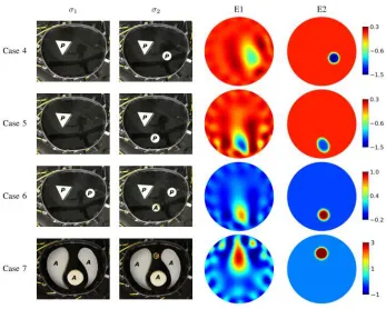
2) Water tank cases: In the phantom experimental studies (Cases 4-7), the experiments were performed using a human thorax-shaped water tank, see Fig.7.L= 16identical metallic rectangular electrodes with a width of 2 cm were attached to the interior lateral surface of the tank. The horizontal and vertical radii of the tank were Rh = 17.5 cm and
Rv = 14 cm, respectively. The tank was filled with tap
water, and objects made of different materials (agar, plastic or copper) were placed inside the tanks to simulate different conductivity distributions. To present the inclusions in an easy-to-read style, the material type of each inclusion was marked by a capital letter, e.g., the inclusion marked by a letter ‘A’ meaning “made from agar”, see details in Fig.7. All inclusions were homogeneous in the vertical direction and extended through the water surface. The measurements were acquired with the KIT4 system [48], using adjacent current stimulation (frequency 10 kHz, amplitude 1 mA) and adjacent measurement.
3) Test cases using pig data: The pig data was collected on anesthetized ventilated supine pigs (mean body weight
30.1±2.3 kg) as part of the study in [32], using the Goe MF II EIT system from University of Gottingen. L = 16 ECG electrodes were placed around the thorax 3 cm below the axilla. Right-sided pneumothorax and pleural effusion were artificially induced by means of manual injection of air up to 300 mL and 300 mL Ringer solution, respectively. To open the pleural cavity for injection of air or fluid, a small surgical incision into the chest wall was made and a plastic cannula was fixed by a suture and sealed by cyanoacrylate glue. For more details, we refer the reader to the paper [32]. The reference data was obtained by averaging voltages data of 120 seconds duration before intervention.
B. Computational domain modeling
• In the simulated cases 1-3, to test the general behavior of our PLS-based difference imaging approach, we assume that the target domain Ω is accurately known, and in the reconstruction, we used the correct domain as the model domain, i.e., Ω = Ω, meaning that no geometric˜ modeling errors are present. However, during clinical measurements, the body shape is not always known, and an approximate model domain Ω˜ has to be employed. Therefore, in the following experimental studies (Cases 4-9), we study the effect of modeling errors caused by inaccurately known shape of the target domain.
• In water tank Cases 4-7, since the inclusions were homo-geneous in the vertical direction and extended through the water surface, a 2D model was adequate for modeling the measurements. In the reconstruction, we used a 2D circle domain with radius 17.5 cm as the model domain shown in Fig.2.
• In the studies (Cases 8&9) using in vivo pig data, we applied a cylinder with radius 11 cm and height 10 cm as the model domain, representing 3D studies using incorrect model domain. Note that, since measurements of the pig chest circumference at the electrode plane were not available, the selection of the cylinder radius was estimated from chest circumferences based on weight information, by using a regression model1with 38 pigs:
chest circumference in cm = 0.992*weight in kg + 36.6 cm. In the model domain, the electrode plane was placed at the half-height (z= 5 cm) of the cylinder.
The discretization details of the target domain are show in Table II.
Fig. 2. Measurement domainΩshown as gray patch and model domainΩ˜
(∂Ω˜ is shown with solid line) are used in Cases 4-7.
1The regression model was kindly provided by Prof. G¨unter Hahn, who
TABLE II
FINITE ELEMENT MESHES FOR THE TEST CASES.NnIS THE NUMBER OF NODES ANDNEIS THE NUMBER OF ELEMENTS(TRIANGULAR ELEMENTS
FORCASES1-7AND TETRAHEDRAL ELEMENTS FORCASES8-9).
Simulation studies Experimental studies Cases 1-3 Cases 4-7 Cases 8-9 Simulated data Reconstruction Reconstruction Reconstruction
Nn 7150 5586 3301 12509
NE 13802 10674 6264 57006
C. Estimates
The following estimates were computed. For parameter choices of each reconstruction, see Section V-D.
• (E1) Conventional linear difference imaging recon-struction of ∆σ by solving:
c
∆σ= arg min∆σ{kL∆e(∆V −J∆σ)k2
+kL∆σ(∆σ−∆σ∗)k2},
(24)
where ∆σ∗ is the expectation of ∆σ, which is usually set to 0. LT∆σL∆σ = Γ∆−1σ, and Γ∆σ is a smoothness
promoting covariance matrix with elements defined as
Γ∆σ(τ, κ) =aexp
−kxτ−xκk
2 2
2b2
+dδτ κ. (25)
Here, Γ∆σ(τ, κ) is a covariance matrix, element (τ, κ)
corresponding to a generic smoothness prior model for the unknown conductivity change ∆σ at the nodes in locations xτ and xκ. Parameters a, b andd are positive
scalar parameters, listed in table III for different test cases, where a can be used to tune the variation of the conductivity change, b sets the correlation length of the model, and d is a small positive value which is used to ensure that Γ∆σ is well-conditioned. The selections
of a, b and d are based on simulations and visual inspection of the results. δτ κ denotes the Kronecker
delta function, where δτ κ = 1 for τ = κand δτ κ = 0,
otherwise. Note that, in estimate (E1), the conductivity change is estimated by treating the internal distribution to be continuous i.e. without considering the piecewise constant assumption. Thus the corresponding unknown parameters vector was (∆σ)T
∈RNn
• (E2) Parametric level set based difference imaging reconstruction: The estimates for the shape and binary conductivity change values were computed by solving the minimization problem as given in (20)
[ˆµ,∆dσ0,∆dσ1] = arg min{kLe(∆V −∆U)k2
+k(µ−µ∗)k2+ P1
j=0k
L∆σj(∆σj)k
2
}, (26)
D. Model implementation
In this section, we discuss important information related the implementation of the proposed imaging approach. To start, we remark that the µ′
is weight coefficients were initially set
to 0.5 for all test cases studied in this paper. We would like
TABLE III
PRIORI PARAMETERS ANDGAUSSIAN WIDTH COEFFICIENT.
Simulated data Water tank data Pig data Cases 1-3 Cases 4-7 Cases 8-9
E1
a 1.5 0.3 10−3
b 1 1 1.6
c 10−3 10−3 10−6
E2 K 1.3 0.2 0.5
to point out that the true values of theµ′
isweight coefficients
are not assumed to be known in a priori; rather, they are estimated numerically. For the shape representation, Heaviside function (14) with ε = A/2 was used, here, A denotes the mean value of the element area/volume in the FEM mesh, i.e., A= Area/volume of domainΩ
Number of elements . A fixed constant c=fm level
set was applied for (17), wherefm is the mean value of the
initial LSF fk. The Cholesky factor L∆σ in (26) or in (20)
is calculated as LT
∆σL∆σ = C∆−σ1, where C∆σ is selected
as
1 0 0 100
. A large variance for ∆σ1 indicates that the
estimated value of∆σ1is spread out far from the initial guess,
while a small variance for∆σ0 indicates the opposite.
Next, we address the selection of the Gaussian width parameter γ for the GRBF (16) in the PLS-based difference imaging approach. As in [42], we rewrite the GRBF (16) in the new form of
pi(x) = exp(−λkx−xik)2. (27)
where, λ= (√2γ)−1. Obviously, by adjusting the parameter
variantλ, the widthγ of GRBF will be changed accordingly. To allow a semi-automated way for choosing this variant λ, we define
λ=KA, (28)
here,K is a free coefficient of the Gaussian width parameter, which is given in Table III.The selection ofK was based on simulations and visual inspection of the results.A robustness study of PLS-based difference imaging approach w.r.t the Gaussian width coefficient K will be discussed in Section VI-A.
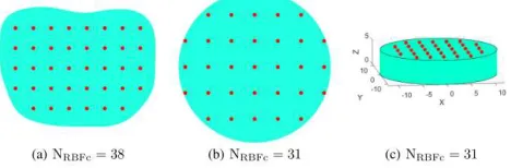
According the work in [42], given a reasonable choice of numbers of RBF centers (NRBFc) and roughly equally
distributed RBF centers xi in the domain to be imaged, the
PLS-based absolute reconstruction method is quite robust to the choice of the initial distribution of xi. In this study,
using the same RBF centers selection strategy in [42], we chose NRBFc = 38 for simulations and NRBFc = 31 for
experimental studies. Thus the corresponding unknown pa-rameters vector was (µ,∆σ0,∆σ1)T ∈ R40 for simulations,
(µ,∆σ0,∆σ1)T ∈R33 for experimental studies. A
presenta-tion image of the distribupresenta-tion of thexifor both numerical and
experimental test cases is shown in Fig 3.
Fig. 3. Distributions of the RBF centersxiused for the PLS-based difference imaging approach.
VI. RESULTS ANDDISCUSSION
We now demonstrate the effect of the PLS-based difference imaging approach on simulated as well as experimental data. To quantitatively evaluate the performance of both estimates (E1&E2), we computed the relative size/volume coverage ratio (RCR) [28], shown in Table IV, for measuring how well the sizes/volumes of inclusions were recovered:
RCR = CR CRTrue
, (29)
where CR measures the coverage ratio defined as the ratio of the size/volume of the inclusions to the total size/volume of the target. Correspondingly, CRTrue is the CR of the true target.
For determining the size/volume of the inclusion, a threshold of half of the maximum/minimum of the ∆cσ was used to detect the inclusion.
Note that for computing the RCRs in Cases 8&9, it is dif-ficult to know the true target volume, therefore we simplified the definition of (29) into
RCR = volume of estimated mass volume of injected mass ,
which indicates how much difference is generated between the estimated volume of the mass (air or fluid) volume and the true mass volume.
Further, the minimum/maximum of the reconstructed con-ductivity changes were used to measure the accuracy of the recovered contrast. The contrasts of the reconstructed con-ductivity changes are tabulated in terms of a relative contrast (RCo)
RCo = max|∆bσ| max|∆σtrue|
.
We should point out that, to compute the RCo values of Cases 4 & 5, we assumed that the conductivity value of plastic bar is zero, such that max|∆σtrue| = σtap water. Note that
neither the conductivity values of the inclusions composed of agar and copper in Cases 6 & 7 nor the conductivity changes in the pig thorax (Cases 8 & 9) were accurately known. Therefore, we didn’t compute the RCo values for those cases. The relative quantities RCR and RCo are used here instead of the respective quantities CR and max|∆bσ| to facilitate the comparison of the values in Table IV. For both RCR and RCo, value of 1 would indicate an exact match of the true and estimated values of the conductivity change, while a value greater or less than 1 would imply overestimation or underestimation, respectively.
In addition, for the simulation studies, we also computed the structural similarity (SSIM) index, see details in [49], for measuring the similarity between the true and reconstructed images. A SSIM value of 1 represents the two compared images are exactly the same, a perfect match, while value of zero indicates little similarity. Note that no SSIMs were computed for experimental test cases since the inclusions are infinite conductors or resistors or the true images are not available.
A. Reconstructions from simulated data
The true conductivity distributions and the estimates (E1&E2) for the simulated test cases 1-3 are shown in Fig.4. The conductivity distributions before (σ1) and after (σ2)
change, and the conductivity change∆σare shown in the first to third columns, respectively. The fourth and fifth columns shows the conventional linear difference imaging (E1) and the proposed PLS-based difference imaging (E2), respectively.
In the estimate (E1), the shape of the changes in Cases 1-3 are recovered relatively well, although there is a clustering of artifacts in the reconstructed images, and the amplitude of reconstructed contrasts of ∆σ are heavily biased. The reconstruction artifacts and contrast distortion are mainly due to the use of an approximatedJ evaluated at a homogeneous conductivityσ0, which is clearly a poor model for the thorax
[33], in which the lungs are far less conductive than the background tissue.
On the other hand, the estimate (E2) with the proposed PLS-based difference imaging approach, in all the numerical test cases, results in good qualitative estimates of the conductivity change ∆σ. This observation is quantitatively confirmed by SSIMs, RCRs and RCos closest to the true values, as given in Table IV. It is worth noticing that in (E2), although the amplitude of reconstructed contrasts of∆σis also biased, the shape of the inclusions is still very feasible for all simulated cases. Especially in Case 3, (E2) provides not only the best shape estimation of the inclusion, which associates evidence with the SSIM value 0.97, but also feasible reconstruction of amplitude contrast of∆σ, as evident from the RCo value 1.01 shown in Table IV.
Overall, the results of the simulated test cases indicate that the PLS-based difference imaging approach improves the accuracy of the estimates of∆σcompared to the conventional linear difference imaging approach, and that the proposed approach tolerates modeling errors caused by the approxima-tion of Jacobian matrix J better than the conventional linear difference imaging.
TABLE IV
THESSIMINDEXES ANDRCRS OF THE RECOVERED INCLUSIONS AND THE RELATIVE CONTRAST VALUE(RCO)OF THE RECONSTRUCTED∆cσ.
Simulated data Water tank data Pig data
Case 1 Case 2 Case 3 Case 4 Case 5 Case 6 Case 7 Case 8 Case 9
[image:9.612.344.530.398.687.2]SSIM RCR RCo SSIM RCR RCo SSIM RCR RCo RCR RCo RCR RCo RCR RCR RCR RCR True 1.00 1.00 1.00 1.00 1.00 1.00 1.00 1.00 1.00 1.00 1.00 1.00 1.00 1.00 1.00 1.00 1.00 E1 0.73 0.56 3.75 0.76 0.52 3.77 0.81 2.93 0.64 2.99 0.58 1.78 0.96 2.53 8.47 2.05 2.45 E2 0.76 0.61 3.43 0.79 0.65 3.24 0.97 0.42 1.01 0.75 1.15 1.08 0.90 0.99 2.30 0.74 1.12
Fig. 4. Reconstructions with both conventional linear difference imaging (E1) and PLS-based difference imaging (E2) approaches from simulated data.
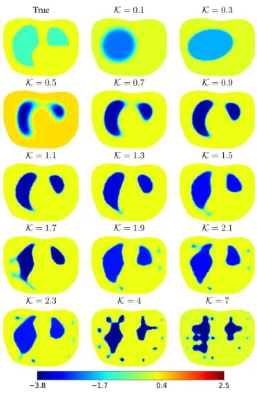
which is due to the fact that a smallK, i.e., a bigγ, for RBF will lose the locality intended for the expected inclusions; With the 3rd smallest K = 0.5, i.e., corresponding to the 3rd largest γ, the estimated image is blurry, which is an expected result, since a large Gaussian width determines a large degree of smoothing–the larger the width, the larger the size of the structures which are smoothed away. Conversely, too large values of K = 4,· · · ,7 (i.e., the values of width γ are too small), produce in narrow-band inclusions around the RBF centers. With all the other selected values of K, the inclusions are relatively well recovered, producing enhanced lung edges, which is also verified by the metrics parameter SSIM indices shown in Fig.6. We note that the coefficient K increasing from 1.7 to 2.3 tends to produce artifacts near the edge of the inclusions, which may be related to a trend that reflects producing edge artifacts. In choosing the Gaussian width parameterγor coefficientK, one always faces a trade-off between ‘edge sharpening’ and ‘artifacts eliminating’.
B. Reconstructions from water tank data
Next, we proceed to reconstructions from water tank data. Fig. 7 depicts the results of both estimates (E1&E2) on four experimental test Cases 4-7. As the results shown in Fig. 7, the conductivity change was detected in both estimates (E1&E2), despite the significant error (see Fig. 2) in the shape of the model domain. However, the accuracy of these reconstructions based on (E1) is rather low, leading a large number of artifacts in the reconstructed images, and especially the shapes of the inclusions are not tracked very well. Consequently, (E1)
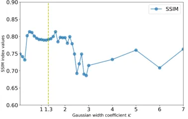
Fig. 5. Robustness study of the PLS-based difference imaging approachw.r.t
Fig. 6. SSIM index versus the Gaussian width parameter coefficient Kin case 2 using the PLS-based difference imaging approach for recovering the conductivity change of the collapsed lung. The dashed vertical line denotes the case shown in the2nd
row of Figure 4.
overestimates the coverage ratio RCRs significantly, see Table IV. On the other hand, (E2) leads to the best estimation of conductivity change for both high contrast (Cases 4,5 and 7) and low contrast experiments (Case 6). (E2) also results in the coverage ratio closest to the true value, e.g., RCR being 0.99 for Case 6, see Table IV. Note that the result of Case 7 indicates that the proposed approach has better potential for the detection of the descending aorta using EIT.
To check how well the estimate (E2) based on the proposed method tolerates the modeling errors, we also computed the reconstructions with (almost) correct domain model for Case 6 in Fig. 8 for a comparison study. As is obvious from the reconstructions in Fig. 8, with or without geometric modeling errors, estimate (E2) produces better reconstructions than estimate (E1). It is also evident from the RCR of the recovered inclusions, e.g., RCR being 2.23 and 1.04 for (E1) and (E2), respectively, in the case of applying (almost) correct domain model for the reconstructions.
C. Reconstructions from pig data
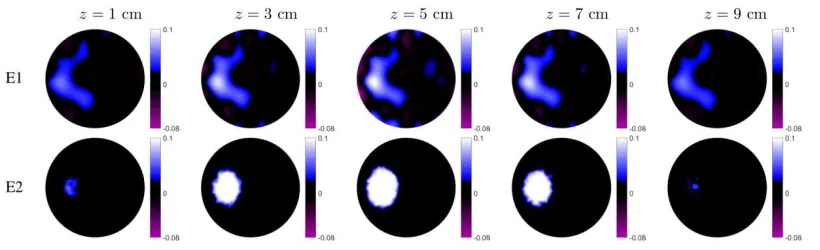
The reconstructions of pig data described in Section V-A3 are shown in Figs. 9 and 10, The slices that are shown, are the horizontal cross sections atz= 1,3,5,7 and 9 cm of the reconstructed 3D conductivity. The slices from ventral (upper) to dorsal (lower) are presented in radiological convention, which means that the left side of the image corresponds to the right side of the pig. Note that in Figs. 9 and 10, we used a colour map developed by Draegerwerk AG & Co. KGaA for display of EIT ventilation images.
Again, both estimates (E1&E2) using the incorrect model domainΩ˜ are able to localize the unilateral right pneumotho-rax and pleural effusion, corresponding to the correct side of injection, in the anesthetized, ventilated pig. More precisely, the region with negative conductivity change after air injection is located at the more ventral part of the images, and after Ringer solution injection, the region with positive conductivity change located in the middle region. Note that the recovered fluid region is represented more dorsally than the air, which is an expected result since the position of fluid accumulation was below that of air accumulation in relation to the effect of gravity in supine pigs. These findings are consistent with those from previous studies [27], [32].
Comparing the reconstructions based on (E1) and (E2), the (E2) based reconstructions show that conductivity changes are more clearly defined and free of artifacts. Estimate (E2) also results in the coverage ratio closest to the true value, RCRs being 0.74 and 1.12 (see Table IV) for Cases 8&9, respectively. Overall, the results of the test cases using pig data indicate that the PLS-based difference imaging approach improves the accuracy of the estimates, resulting superior visual quality of the conductivity change, as is evident from the metric parameter RCR, compared to that obtained by conventional linear difference imaging approach.
D. Discussion on the results
Difference EIT has been well known to tolerate modeling errors caused by inaccuracies in modeling target domains. To some extent, this feature is observed in the results reported herein. In all cases, the estimate (E1) is, at least, indicative of the location of the conductivity change. Although the conventional linear difference imaging approach is able to suppress some of the effects of modeling errors, it has been shown that a large number of artifacts are still present in the reconstructions, which is mainly due to the fact that the sensitivity distribution in the domain is affected by the selection of a homogeneous conductivity distribution σ0 for
evaluating Jacobian matrixJ.
On the other hand, the proposed PLS-based approach is much less affected by modeling errors, caused by inaccurately known domain geometry and the poorly approximated sensi-tivity distribution, than that of the conventional linear differ-ence imaging approach. This is probably due to the fact that, in the PLS-based approach, the conductivity change was assumed to be piecewise constant and the geometry of the anomaly was represented by a shape-based PLS function using a low order representation. The allows reducing dramatically the overall number of unknowns, improving the condition number of the inverse problem, and enhancing the computational efficiency of the technique. Meantime, the PLS-based reconstruction problem was solved iteratively, offering a greater chance of arriving at an more accurate reconstruction of the problem.
Finally, we discuss computational aspects pertinent to the efficiency of the reconstruction algorithm. It is well known that, in the traditionally used pixel/voxel-based non-linear iterative methods [46], a line search is usually performed on the conductivity update. This process demands repetitive calculation of the forward problem, which becomes a severe bottleneck [50]. For example, the use of non-linear iterative methods coupled with a line search takes several minutes [51] to obtain the final reconstructions. In contrast, conventional linear difference approaches are known to be computationally fast since iteration is not needed. As an example, the estimate (E1) shown in Fig. 7 was obtained from a MATLAB imple-mentation of the conventional linear difference approach on a desktop PC with an Intel Core i7-6700K processor and 32GB memory within 6 to 8.5 seconds.
[image:10.612.81.270.58.178.2]Fig. 7. Reconstructions with both conventional linear difference imaging (E1) and PLS-based difference imaging (E2) approaches from water tank data. The letters ‘A’, ‘C’ and ‘P’ marked in the phantom photos denote the inclusions which were made of agar, copper and plastic materials, respectively.
Fig. 8. Reconstructions with both conventional linear difference imaging (E1) and PLS-based difference imaging (E2) approaches for Case 6 using (almost) correct domain model (1st row) and approximated circle domain model (2nd row). The 2nd row is a repetition of the 3rd row from Fig. 7.
Fig. 9. Reconstructed images of the right-sided pneumothorax. (E1): estimates based on the conventional linear difference imaging. (E2): the proposed PLS-based difference imaging reconstructions.
[image:11.612.104.507.556.680.2]Fig. 10. Reconstructed images of the right-sided pleural effusion. (E1): estimates based on the conventional linear difference imaging. (E2): the proposed PLS-based difference imaging reconstructions.
demonstration of this realization, the final reconstructions shown in Fig. 7 were obtained from aMATLABimplementation of the proposed approach on the above PC within 5 to 10 sec-onds. The CPU time of the proposed approach is comparable to the conventional linear difference approach. Compared to the traditional pixel/voxel-based non-linear iterative methods, the reduced computing times of the proposed approach allows for faster reconstruction of EIT images enabling improved interaction. This positively impacts opportunities for exploring different data sets with EIT and may provide better insight to a large suite of data by experimenting with different reconstruction parameters.
VII. CONCLUSION
In this paper, we proposed a parametric level set based difference imaging approach for reconstructing the conductiv-ity change in EIT. The proposed approach was evaluated by simulations, phantom studies and in vivo pig data. We found that the PLS-based approach provides more accurate recon-structions of the conductivity change than the conventional linear difference approach. It has been shown that the proposed approach tolerates modeling errors caused by inaccurately known domain geometry, as well as the poorly approximated sensitivity distribution. The findings demonstrate that, given the assumption that the properties of conductivity change are piecewise constant, the proposed approach is not only robust, but also compare favorably with the linear difference approach.
ACKNOWLEDGMENT
The authors would like to thank UEF inverse problems group, for providing us with the FEM codes used for the forward solution of the EIT problem. The authors would also like to thank Prof. G¨unter Hahn for sharing the pig data.
REFERENCES
[1] K. Y. Aristovich, B. C. Packham, H. Koo, G. S. dos Santos, A. McEvoy, and D. S. Holder, “Imaging fast electrical activity in the brain with electrical impedance tomography,”NeuroImage, vol. 124, pp. 204–213, 2016.
[2] C. N. Herrera, M. F. Vallejo, J. L. Mueller, and R. G. Lima, “Direct 2-d reconstructions of conductivity and permittivity from eit data on a human chest,”IEEE transactions on medical imaging, vol. 34, no. 1, pp. 267–274, 2015.
[3] I. Frerichs, M. B. Amato, A. H. van Kaam, D. G. Tingay, Z. Zhao, B. Grychtol, M. Bodenstein, H. Gagnon, S. H. B¨ohm, E. Teschneret al., “Chest electrical impedance tomography examination, data analysis, terminology, clinical use and recommendations: consensus statement of the translational eit development study group,”Thorax, pp. thoraxjnl– 2016, 2016.
[4] L. Zhou, B. Harrach, and J. K. Seo, “Monotonicity-based electrical impedance tomography for lung imaging,” Inverse Problems, vol. 34, no. 4, p. 045005, 2018.
[5] E. K. Murphy, A. Mahara, and R. J. Halter, “Absolute reconstructions using rotational electrical impedance tomography for breast cancer imaging,”IEEE Transactions on Medical Imaging, vol. 36, 4 2017. [6] K. H. Wodack, S. Buehler, S. A. Nishimoto, M. F. Graessler, C. R.
Behem, A. D. Waldmann, B. Mueller, S. H. B¨ohm, E. Kaniusas, F. Th¨urk
et al., “Detection of thoracic vascular structures by electrical impedance tomography: a systematic assessment of prominence peak analysis of impedance changes,”Physiological measurement, 2018.
[7] D. Liu, V. Kolehmainen, S. Siltanen, and A. Sepp¨anen, “A nonlinear approach to difference imaging in eit; assessment of the robustness in the presence of modelling errors,”Inverse Problems, vol. 31, no. 3, p. 035012, 2015.
[8] A. Nissinen, V. P. Kolehmainen, and J. P. Kaipio, “Compensation of modelling errors due to unknown domain boundary in electri-cal impedance tomography,” IEEE Transactions on Medical Imaging, vol. 30, no. 2, pp. 231–242, 2011.
[9] M. Hanke and M. Br¨uhl, “Recent progress in electrical impedance tomography,”Inverse Problems, vol. 19, no. 6, p. S65, 2003. [10] B. Gebauer and N. Hyv¨onen, “Factorization method and irregular
inclu-sions in electrical impedance tomography,”Inverse Problems, vol. 23, no. 5, p. 2159, 2007.
[11] B. Harrach, “Recent progress on the factorization method for electrical impedance tomography,”Computational and mathematical methods in medicine, vol. 2013, 2013.
[12] A. Kirsch, “Characterization of the shape of a scattering obstacle using the spectral data of the far field operator,”Inverse problems, vol. 14, no. 6, p. 1489, 1998.
[13] A. Abbasi and B. V. Vahdat, “A non-iterative linear inverse solution for the block approach in eit,” Journal of Computational Science, vol. 1, no. 4, pp. 190–196, 2010.
[14] S. Siltanen, J. Mueller, and D. Isaacson, “An implementation of the reconstruction algorithm of a nachman for the 2d inverse conductivity problem,”Inverse Problems, vol. 16, no. 3, p. 681, 2000.
[15] J. L. Mueller, S. Siltanen, and D. Isaacson, “A direct reconstruction algorithm for electrical impedance tomography,”IEEE Transactions on medical imaging, vol. 21, no. 6, pp. 555–559, 2002.
[16] K. Knudsen, M. Lassas, J. L. Mueller, and S. Siltanen, “Regularized d-bar method for the inverse conductivity problem,”Inverse Problems and Imaging, vol. 35, no. 4, p. 599, 2009.
[17] A. Hauptmann, M. Santacesaria, and S. Siltanen, “Direct inversion from partial-boundary data in electrical impedance tomography,”Inverse Problems, vol. 33, no. 2, p. 025009, 2017.
[18] M. Alsaker, S. J. Hamilton, and A. Hauptmann, “A direct d-bar method for partial boundary data electrical impedance tomography with a priori information,”Inverse Problems & Imaging, vol. 11, no. 3, pp. 427–454, 2017.
[20] J. L. Mueller and S. Siltanen, Linear and nonlinear inverse problems with practical applications. Siam, 2012, vol. 10.
[21] D. Isaacson, J. Mueller, J. Newell, and S. Siltanen, “Imaging cardiac activity by the d-bar method for electrical impedance tomography,”
Physiological Measurement, vol. 27, no. 5, p. S43, 2006.
[22] E. K. Murphy and J. L. Mueller, “Effect of domain shape modeling and measurement errors on the 2-d d-bar method for eit,”IEEE transactions on medical imaging, vol. 28, no. 10, pp. 1576–1584, 2009.
[23] S. Hamilton, “Eit imaging of admittivities with a d-bar method and spatial prior: experimental results for absolute and difference imaging,”
Physiological measurement, vol. 38, no. 6, p. 1176, 2017.
[24] M. Dodd and J. L. Mueller, “A real-time d-bar algorithm for 2-d electrical impedance tomography data,”Inverse problems and imaging (Springfield, Mo.), vol. 8, no. 4, p. 1013, 2014.
[25] M. Cheney, D. Isaacson, J. C. Newell, S. Simske, and J. Goble, “Noser: An algorithm for solving the inverse conductivity problem,”
International Journal of Imaging Systems and Technology, vol. 2, no. 2, pp. 66–75, 1990.
[26] B. H. Brown and A. D. Seagar, “The sheffield data collection system,”
Clinical Physics and Physiological Measurement, vol. 8, no. 4A, p. 91, 1987.
[27] A. Adler, J. H. Arnold, R. Bayford, A. Borsic, B. Brown, P. Dixon, T. J. Faes, I. Frerichs, H. Gagnon, Y. G¨arberet al., “Greit: a unified approach to 2d linear eit reconstruction of lung images,”Physiological measurement, vol. 30, no. 6, p. S35, 2009.
[28] D. Liu, V. Kolehmainen, S. Siltanen, A.-M. Laukkanen, and A. Sepp¨anen, “Nonlinear difference imaging approach to three-dimensional electrical impedance tomography in the presence of geo-metric modeling errors,”IEEE Transactions on Biomedical Engineering, vol. 63, no. 9, pp. 1956–1965, 2016.
[29] A. Adler, R. Guardo, and Y. Berthiaume, “Impedance imaging of lung ventilation: do we need to account for chest expansion?”IEEE transactions on Biomedical Engineering, vol. 43, no. 4, pp. 414–420, 1996.
[30] A. Boyle, A. Adler, and W. R. Lionheart, “Shape deformation in two-dimensional electrical impedance tomography,”Medical Imaging, IEEE Transactions on, vol. 31, no. 12, pp. 2185–2193, 2012.
[31] D. Holder and A. Khan, “Use of polyacrylamide gels in a saline-filled tank to determine the linearity of the sheffield mark 1 electrical impedance tomography (eit) system in measuring impedance distur-bances,”Physiological measurement, vol. 15, no. 2A, p. A45, 1994. [32] G. Hahn, A. Just, T. Dudykevych, I. Frerichs, J. Hinz, M. Quintel, and
G. Hellige, “Imaging pathologic pulmonary air and fluid accumulation by functional and absolute eit,”Physiological measurement, vol. 27, no. 5, p. S187, 2006.
[33] B. Grychtol and A. Adler, “Uniform background assumption produces misleading lung eit images,”Physiological measurement, vol. 34, no. 6, p. 579, 2013.
[34] T. Tallman, S. Gungor, K. Wang, and C. Bakis, “Damage detection and conductivity evolution in carbon nanofiber epoxy via electrical impedance tomography,”Smart Materials and Structures, vol. 23, no. 4, p. 045034, 2014.
[35] F. Gibou, R. Fedkiw, and S. Osher, “A review of level-set methods and some recent applications,”Journal of Computational Physics, 2017. [36] E. T. Chung, T. F. Chan, and X.-C. Tai, “Electrical impedance
tomog-raphy using level set representation and total variational regularization,”
Journal of Computational Physics, vol. 205, no. 1, pp. 357–372, 2005. [37] M. Soleimani, O. Dorn, and W. R. Lionheart, “A narrow-band level set method applied to eit in brain for cryosurgery monitoring,”IEEE transactions on biomedical engineering, vol. 53, no. 11, pp. 2257–2264, 2006.
[38] M. Soleimani, W. Lionheart, and O. Dorn, “Level set reconstruction of conductivity and permittivity from boundary electrical measurements using experimental data,”Inverse problems in science and engineering, vol. 14, no. 2, pp. 193–210, 2006.
[39] D. Liu, A. K. Khambampati, S. Kim, and K. Y. Kim, “Multi-phase flow monitoring with electrical impedance tomography using level set based method,”Nuclear Engineering and Design, vol. 289, pp. 108–116, 2015. [40] A. Aghasi, M. Kilmer, and E. L. Miller, “Parametric level set methods for inverse problems,”SIAM Journal on Imaging Sciences, vol. 4, no. 2, pp. 618–650, 2011.
[41] F. Larusson, S. Fantini, and E. L. Miller, “Parametric level set reconstruc-tion methods for hyperspectral diffuse optical tomography,”Biomedical optics express, vol. 3, no. 5, pp. 1006–1024, 2012.
[42] D. Liu, A. K. Khambampati, and J. Du, “A parametric level set method for electrical impedance tomography,”IEEE Transactions on Medical Imaging, vol. 37, no. 2, pp. 451–460, 2018.
[43] E. Somersalo, M. Cheney, and D. Isaacson, “Existence and uniqueness for electrode models for electric current computed tomography,”SIAM Journal on Applied Mathematics, vol. 52, no. 4, pp. 1023–1040, 1992. [44] P. Vauhkonen, M. Vauhkonen, T. Savolainen, and J. Kaipio, “Three-dimensional electrical impedance tomography based on the complete electrode model,” IEEE Trans. Biomed. Eng, vol. 46, pp. 1150–1160, 1999.
[45] G. Pingen, M. Waidmann, A. Evgrafov, and K. Maute, “A parametric level-set approach for topology optimization of flow domains,” Struc-tural and Multidisciplinary Optimization, vol. 41, no. 1, pp. 117–131, 2010.
[46] D. Liu, V. Kolehmainen, S. Siltanen, A. M. Laukkanen, and A. Sepp¨anen, “Estimation of conductivity changes in a region of interest with electrical impedance tomography,”Inverse Problems and Imaging, vol. 9, no. 1, pp. 211–229, 2015.
[47] C. Gabriel, A. Peyman, and E. Grant, “Electrical conductivity of tissue at frequencies below 1 mhz,”Physics in medicine and biology, vol. 54, no. 16, p. 4863, 2009.
[48] J. Kourunen, T. Savolainen, A. Lehikoinen, M. Vauhkonen, and L. Heikkinen, “Suitability of a pxi platform for an electrical impedance tomography system,” Measurement Science and Technology, vol. 20, no. 1, p. 015503, 2009.
[49] Z. Wang, A. C. Bovik, H. R. Sheikh, and E. P. Simoncelli, “Image quality assessment: from error visibility to structural similarity,”IEEE transactions on image processing, vol. 13, no. 4, pp. 600–612, 2004. [50] J. Fritschy, L. Horesh, D. S. Holder, and R. Bayford, “Using the grid to
improve the computation speed of electrical impedance tomography (eit) reconstruction algorithms,”Physiological measurement, vol. 26, no. 2, p. S209, 2005.