City, University of London Institutional Repository
Citation
:
Zolotas, A.C. & Halikias, G. (1999). Optimal design of PID controllers using the QFT method. IEEE Proceedings - Control Theory and Applications, 146(6), pp. 585-589. doi: 10.1049/ip-cta:19990746This is the accepted version of the paper.
This version of the publication may differ from the final published
version.
Permanent repository link:
http://openaccess.city.ac.uk/16900/Link to published version
:
http://dx.doi.org/10.1049/ip-cta:19990746Copyright and reuse:
City Research Online aims to make research
outputs of City, University of London available to a wider audience.
Copyright and Moral Rights remain with the author(s) and/or copyright
holders. URLs from City Research Online may be freely distributed and
linked to.
arXiv:1211.5494v1 [cs.SY] 23 Nov 2012
Optimal design of PID controllers using the QFT method
A. C. Zolotas
1and G. D. Halikias
2Abstract: An optimisation algorithm is proposed for designing PID controllers, which minimises the asymptotic open-loop gain of a system, subject to appropriate robust-stability and performance QFT constraints. The algorithm is simple and can be used to automate the loop-shaping step of the QFT design procedure. The effectiveness of the method is illustrated with an example.
Keywords: QFT; PID control; Robust control.
1
Introduction
Many practical systems are characterised by high uncertainty which makes it difficult to maintain good stability-margins and performance properties for the closed-loop system. There are two general design methodologies for dealing with the effects of uncertainty: (i) Adaptive control, in which the parameters of the plant (or some other appropriate structure) are identified on-line and the information obtained is then used to “tune” the controller, and (ii)Robust control, which typically involves a “worst-case” design approach for a family of plants (representing the uncertainty) using a single fixed controller.
Quantitative Feedback Theory(QFT) is a robust-control method developed during the last two decades which deals with the effects of uncertainty systematically. It has been sucessfully applied to the design of both SISO and MIMO systems, while the theory has also been extended to the nonlinear and the time-varying case. In comparison to other optimisation-based robust control methods, QFT offers a number of advantages. These include, (i) the ability to assess quantitatively the “cost of feedback” [3], [4], [5], (ii) the ability to take into account phase information in the design process (which is lost if, e.g. singular values are used as the design parameters), and , (iii) the ability to provide “design transparency”, i.e. clear tradeoff criteria between controller complexity and feasibility of the design objectives. Note that (iii) implies in practice that QFT often results in simple controllers which are easy to implement.
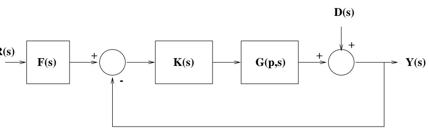
For the purposes of QFT, the feedback system is normally described by the two-degrees-of-freedom structure shown in Figure 1. In this diagram, G(s) is the uncertain plant,K(s) is the feedback controller andF(s) is the pre-filter. The objective is to design
1 Department of Electronic and Electrical Engineering, Control Group, Loughborough University, Loughborough, LE11 3TU, UK
K(s) andF(s) so that the output signalY(s) tracks accurately the reference signalR(s) and rejects the disturbance D(s), despite the presence of uncertainty in G(s).
F(s) R(s)
G(p,s)
K(s) Y(s)
D(s)
+ + +
-Figure 1: Two degree of freedom feedback system
The uncertain plant G(s) is assumed to belong to a set, G(s) ∈ {G(p, s) : p ∈ P}, wherepis the vector of uncertain parameters; these are assumed to be fixed but unknown, and to take values in P. The uncertain plant is first translated in the frequency domain (using a discrete grid of frequenciesω1, ω2, ..., ωN, typically chosen to cover adequately the
system’s bandwidth), resulting in N “uncertainty templates” Gi = {G(p, jωi) : p ∈ P},
i = 1,2, ..., N. The tracking specifications are given in the form of upper (Bu(ωi)) and
lower (Bl(ωi)) bounds in the frequency domain, usually based on simple second-order
models to represent appropriate underdamped and overdamped conditions. A similar procedure is followed to formulate the disturbance-rejection objectives of the design: In this case, the magnitude of the sensitivity function|S(p, jωi)|=|(1 +G(p, jωi)K(jωi))−1|
is required not to exceed an appropriate bound Du(ωi) for all i = 1,2, ..., N and every
p ∈ P. Note that the disturbance bounds are defined independently of the tracking bounds due to the presence of the prefilter,F(s).
Next, the tracking and disturbance-rejection specifications are translated to certain conditions on the nominal open-loop frequency response Lo(jω) = Go(jω)K(jω) where
Go(jω) denotes the nominal plant, defined for any p ∈ P. Consider first the tracking
bounds. For each frequency ωi,i= 1,2, ..., N, the tracking specifications will be satisfied
if and only if,
maxp∈P∆
G(p, jωi)K(jωi)
1 +G(p, jωi)K(jωi)
db
≤δ(ωi) :=Bu(ωi)|db−Bl(ωi)|db (1)
i.e. if and only if the maximum variation in the closed-loop gain aspvaries over the setP, at each frequency ωi does not exceed the maximum allowable spread in the specifications
δ(ωi). This is because, (i) the uncertainty associated withKis assumed negligible, and (ii)
the actual closed-loop gain can always be adjusted to its required level at each frequency via the scaling action of the prefilter. For each frequency ωi, the open-loop gain (for
[image:3.612.95.527.111.244.2]the specified robust tracking specifications at frequency ωi. In practice, each “Horowitz
template” is calculated via a bisection algorithm over a phase grid, and the equality condition in (1) is satisfied within a given tolerance. In total, we have N Horowitz templates, one for each frequency of interest ωi. A similar procedure will result in N
robust disturbance-rejection contours,di(ωi, φ),i= 1,2, ..., N, which define the minimum
open-loop gain required to achieve robust disturbance rejection (i.e. disturbance rejection for every p ∈ P). Clearly, to achieve robust tracking and robust disturbance-rejection
simultaneously, the open-loop frequency response must satisfy,
|L(jωi)| ≥fi(ωi, φ) := max{hi(ωi, φ), di(ωi, φ)} (2)
for alli= 1,2, ..., N, where the maximum in (2) is calculated pointwise inφ = argL(jωi).
The contoursfi(ωi, φ) will be referred to as the robust-performance bounds.
In addition to robust-performance objectives, the closed-loop system should also be robustly stable, i.e. the closed-loop transfer functionF(s)G(p, s)K(s)(1 +G(p, s)K(s))−1
should be stable for every p ∈ P. Since F(s) will be designed stable, robust stability can be inferred from the number of encirclements around the −1 point by the open-loop frequency response L(p, jω) = G(p, jω)K(jω), p ∈ P. In practice, a more severe constraint is imposed on L(p, jω): To establish a minimum amount of damping for the (nominal) closed-loop system, the nominal open-loop response is constrained not to enter anM-circle of an appropriate value. Under the assumption of parametric uncertainty1 in the plant, the uncertainty templates ofGo(jω) at high frequencies approach a vertical line
in the Nichols chart. Hence, to ensure that the specified minimum amount of damping is maintained at high frequencies despite the presence of uncertainty, the M circle is translated downwards by a specific amount, resulting in the so-called “universal high frequency boundary”, which should not be penetrated by the nominal open-loop response [4]. This contour will be denoted by B in the sequel.
2
Optimal Design of PID controllers
After constructing the contoursfi(ωi, φ) and Bon the Nichols’ chart, QFT normally
pro-ceeds with the design of the feedback controller K(s). This normally involves frequency-shaping of the nominal open-loop frequency responseLo(jω), so that it does not penetrate
the the B contour and |Lo(jωi)| lie on or above the robust-performace bounds fi(jωi, φ)
for each ωi. At this stage, the designer normally follows a phase-lead/lag compensation
approach which involves a considerable trial-and-error element, and can be cumbersome, especially if the number of specified frequencies is large and the specifications are tight. If the specifications can not be achieved, the design objectives are assumed to be infea-sible. In this case, the specifications are normally relaxed and the design is repeated. If
the specifications are feasible, the best design is considered to be the one for which the specifications are met as tightly as possible. This is in order to avoid the possibility of “overdesigning” the system using unnecessarily large gains/bandwidth, which can result in measurement noise amplification and potential instability due to parasitics and high-frequency unmodelled dynamics [3], [4]. A compromise between controller complexity and a “tight” design has to be made in many cases.
In this section we present a simple algorithm for designing PID controllers which are optimal in the QFT sense. PID (or “three-term”) controllers are widely used in industry because they are simple and easy to tune. Our algorithm can be used to provide an adequate QFT design, or as the first step for designing a more complex controller [1]. In addition, the algorithm can easily tackle a large number of constraints and can be also be applied to multivariable systems, using the standard QFT approach [7], [6].
A PID controller has a transfer function,
Kpid(s) =kp+
ki
s +kds (3)
and is therefore completely defined by the three termskp (proportional gain),ki (integral
gain) and kd (derivative gain). Its frequency response is
Kpid(jω) =kp−j
ki
ω +jkdω (4)
Suppose thatKpid(s) is used in cascade with an uncertain plantG(p, s). Then, the nominal
open-loop system has frequency responseLo(jω) =Go(jω)Kpid(jω), whereGo(s) denotes
the nominal plant. Thus, the asymptotic gain of the nominal open loop system is given by,
limω→∞
Go(jω) kp−j
ki
ω +jkdω
!
(5)
Suppose that the asymptotic gain of the nominal plant is |Go(jω)| ∼ Aω−p where the
pole/zero excess of the nominal plant p is at least equal to 2. Then the asymptotic gain of the nominal open loop is|Lo(jω)| ∼A|kd|ω−p+1. Since A and p are fixed, the nominal
open-loop gain at high frequencies is minimised by minimising |kd|. This objective is
consistent with the aims of QFT theory outlined previously.
To design an optimal PID controller, consistent with the requirements of QFT, we formulate the following optimisation problem:
Minimise|kd|subject to the constraints:
1. |Lo(jωi)| ≥fi(ωi, φ) for all i= 1,2, ..., N where φ:= argLo(jωi).
2. Lo(jωi)∈ B/ for all i= 1,2, ..., N.
as long as fi(ωi, φi) intersects B or lies entirely above it, by calculating the point-wise
maximum of the two contours in the common phase range. This is almost always the case in practice, since robust performance objectives are almost never associated with frequencies significantly exceeding the closed-loop bandwidth. The (unlikely) case that a performance bound lies below theBcontour can also be accomodated in our algorithm via an additional checking condition. To simplify the presentation, however, we will assume in the sequel that this does not occur, and the combined contours will be denoted by
˜
fi(ωi, φi). The optimisation problem, therefore, takes the form: Minimise |kd| subject to
|L(jωi)| ≥f˜i(ωi, φ) for all i= 1,2, ..., N.
The magnitude (linear) and phase ofKpid(jω) are given by,
|Kpid(jω)|=
v u u tk2
p + kdω−
ki
ω
!2
, arg(Kpid(jω)) :=ψ(ω) = tan−1
kdω−kωi
kp
! (6)
respectively. Now suppose that we fix the phase ofKpid at two distinct frequenciesωi and
ωj, i.e. ψ(jωi) =ψi and ψ(jωj) =ψj. Then,
ψ(jωi) =ψi = tan−1
kdωi− kωii
kp
(7)
which implies that
kd−
ki
ω2 i
− kptan(ψi)
ωi
= 0 (8)
Similarly,
kd−
ki
ω2 j
− kptan(ψj)
ωj
= 0 (9)
Equations (8) and (9) can be arranged in matrix form as:
1 −ω12
i −
tan(ψi)
ωi
1 −ω12
j −
tan(ψj)
ωj kd ki kp
= 0 (10)
Denote the 2×3 matrix in equation (10) byA(ψi, ψj). Clearly, Rank(A(ψi, ψj)) = 2 since
ωi 6= ωj. Therefore, the kernel of A(ψi, ψj) is a one-dimensional subspace of R3, which
implies that the controller gains kd, ki and kp are fixed up to scaling. Numerically, the
kernel ofA(ψi, ψj) can be calculated easily using the Singular Value Decomposition.
Applying the Singular Value Decomposition to A(ψi, ψj) gives:
A(ψi, ψj) =
U1 U2
σ1 0 0
0 σ2 0
VT 1 VT 2 (11)
whereVT
1 is a 2×3 matrix. HereV2spans the kernel ofA(ψi, ψj). WriteV2T = [V21V22V23].
Then, kd ki kp =λ
where λ is an arbitrary real constant. Using equation (6), the gain and phase of Kpid(s)
may be written as
|Kpid(jω)|=|λ|
s
V2
23+
V21ω−
V22
ω
2
, ψ(ω) = tan−1 V21ω−
V22
ω
V23
!
(13)
Note that equation (13) implies that fixing the phase ofKpid(jω) at two frequencies, fixes
the phase ofKpid(jω) atanyfrequency ω, and thus also the phase ofLo(jω). In this case,
minimising|kd| is equivalent to minimising |λV21|.
Under the constraint that ψ(ωi) = ψi and ψ(ωj) = ψj, the QFT constraints are
satisfied if and only if
|Lo(jωk)|db ≥f˜k(ωk, φk) (14)
for allk = 1,2, ..., N, whereφk = arg(Lo(jωk)). Note that since the phase of Kpid(jω) is
fixed at every frequency ω, φk is fixed and knownfor all k = 1,2, ..., N. In fact,
φk = arg(Go(jωk)) + tan−1
V21ωk− Vω22k
V23
(15)
Since,
|Lo(jωk)|db =|Go(jωk)|db+|Kpid(jωk)|db (16)
equation (14) is equivalent to
|Kpid(jωk)|db ≥f˜k(ωk, φk)− |Go(jωk)|db (17)
for all k= 1,2, ...N. Substituting from (13) shows that this is equivalent to
20log10|λ| ≥maxk=1,2,...,N f˜k(ωk, ψk)− |Go(jωk)|db−10log10 V232 +
V21ωk−
V22
ωk
2!!
(18) or|λ| ≥1020β where we have defined,
β = maxk∈{1,2,...N} f˜k(ωk, φk)− |Go(jωk)|db−10log10 V232 +
V21ωk−
V22
ωk
2!! (19)
Multiplying by |V21| and noting that |kd| =|λV21|, implies that |kd| ≥ |V21|10
β
20. Hence,
provided that the phase of Kpid is fixed as arg(Kpid(jωi)) =ψi and arg(Kpid(jωj)) =ψj,
the minimum value of|kd|which achieves the robust-performance constraints is given by
|k∗
d| =|V i,j
2110
βi,j
20 |, where the additional indexes (i, j) introduced in V
21 and β emphasise
the dependence of these variables on (ωi, ωj) and (ψi, ψj). We can now formulate the
following algorithm for solving the optimisation problem. In this algorithm, the gains
ki, kd and kp have been further constrained to be non-negative. This assumption can be
removed, if desired, with minor modifications to the algorithm.
Algorithm 1: Given the plant’s uncertainty templatesGi, a nominal plantGo(jωi)∈
Gi and QFT contraint bounds ˜fi(ωi, φ), each defined at frequencies ω1, ω2, ..., ωN, the
following algorithm calculates an optimal PID controller K∗
pid(s) = k∗p +
k∗
i
s +k
∗
ds with
1. Obtain a phase array Φ by discretising the phase interval (−360◦,0◦).
2. Select any two distinct frequencies ωk, ωl ∈ {ω1, ω2, ..., ωN}.
3. Caclulate phase intervals Φk,Φl ⊆Φ in which the nominal open-loop phase can vary
at ωk and ωl if a PID controller is used. Φk (Φl) contains the phases of Φ which lie
within ±90◦ of the nominal plant phase G
o(jωk) (Go(ωl)).
4. Initialise m×n arrays Kp, Ki and Kd, where m and n are the sizes of Φk and Φl
respectively.
5. For each (Φk(i),Φl(j))∈Φk×Φl
(a) Calculate ψi = Φk(i)−arg(Go(ωk)) andψj = Φl(j)−arg(Go(ωl)).
(b) Calculate the singular value decomposition ofA(ψi, ψk) and the corresponding
vector V2i,j spanning its kernel.
(c) If any two elements ofV2i,j have opposite signs, set Kd(i, j) =∞; Else, let q be
the (common) sign of the elements of V2i,j, calculate βi,j using equation (17),
and set λ=q10βi,j20 , K
d(i, j) =λV21i,j, Ki(i, j) = λV22i,j and Kp(i, j) =λV23i,j.
6. Calculate (i∗, j∗) ∈ argmin
i,jKd(i, j). If Kd(i∗, j∗) = ∞, the constraints cannot be
satisfied by a PID controller with non-negative gains; otherwise the optimal PID controller is K∗(s) = K
p(i∗, j∗) +Ki(i∗, j∗)s−1+Kd(i∗, j∗)s.
Remarks on Algorithm 1:
• In step 1 the phase discretisation of the interval (−360◦,0◦) results in a grid of
phases, typically equally-spaced. In practice, 50-100 phases are adequate. It is helpful to calculate the performance bounds over the same phase grid (Φ).
• In principle any two frequencies ωk,ωl can be selected in step 2. Selecting these two
frequencies reasonably far apart works well in practice.
• In step 3, the phase intervals Φk and Φl may be further restricted, if desired, to
en-sure that the nominal open-loop frequency responseLo(jω) is shaped appropriately.
This will also reduce the number of calculations in step 5 of the algorithm.
• The singular value decomposition in step 5(b) of the algorithm can be dispensed with altogether, by calculating V2i,j analytically. This, however, increases the complexity
of the algorithm and does not lead to any significant reduction in computation time.
• Step 5(c) of the algorithm requires the calculation of βi,j which in turn relies on the
Φ). There is no difficulty, however, in estimating the performance bounds for these phases using the adjacent phase points, e.g. via linear interpolation. Alternatively, the performance bounds can be calculated exactly for the phases obtained from equation (15) via a bisection algorithm implemented between steps 5(a) and 5(c).
• The algorithm can be specialised, if desired, to calculate optimal PI of PD con-trollers. This requires only a one-dimensional search over a phase grid defined at a single frequency.
3
Example
In this section we illustrate our algorithm by means of a simple example. The uncertain plant is taken as
G(s) = ka
s2 +as (20)
in which the parameters a and k vary independently in the intervals 1 ≤ a ≤ 10 and 1≤k ≤10 respectively. The nominal plant, Go(s), is taken to correspond to a = 1 and
k= 1. The tracking specifications are defined as:
|Bl(jωi)| ≤ |T(a, k, jωi)| ≤ |Bu(jωi)| (21)
HereT(a, k, s) =F(s)G(a, k, s)K(s)(1+G(a, k, s)K(s))−1is the closed-loop transfer
func-tion and the lower and upper tracking bounds are defined as the magnitude frequency responses of the two systems
Bl(s) =
0.6585(s+ 30)
(s+ 2 +j3.969)(s+ 2−j3.969) (22)
and
Bu(s) =
8400
(s+ 3)(s+ 4)(s+ 10)(s+ 70) (23) at each s =jωi. Note that the zero of Bl(s) (s = −30) and the two fast poles in Bu(s)
(s = −10 and s =−70) have been included to ensure that the the magnitude frequency responses of Bl(s) and Bu(s) diverge at high frequencies [2]. The frequencies of interest
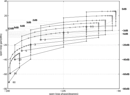
{ωi}have been selected asω1 = 0.5,ω2 = 1,ω3 = 2, ω4 = 3,ω5 = 5,ω6 = 10,ω7 = 30 and
ω8 = 60 rads/s. For simplicity, no disturbance-rejection objectives have been considered
in this example.
−180 −135 −90 −80
−60 −40 −20 0 20 40
−80dB
open loop phase(degrees)
open loop gain(dBs)
−60dB −40dB −20dB −6dB −3dB 0dB
2dB 3dB 6dB 9dB
12dB 0.5
1
2
3
5
10
30
[image:10.612.92.508.79.384.2]60
Figure 2: Uncertainty templates
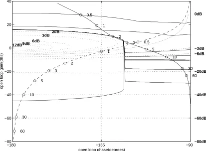
Next, an optimal PID controller was designed following the procedure of Algorithm 1. The optimal controller was obtained as
Kpid∗ (s) = 12.6 + 3.95s+4.46
s (24)
Figure 3 shows the frequency response of the nominal plant (dashed line) and the nominal open loop (solid line) on the Nichols chart, together with the eight Horowitz templates and theB-contour (corresponding to an M value of 1.2). The eight frequencies of interest are indicated by circles on the two frequency responses. The design meets the specifications, since the nominal frequency response does not penetrate theB-contour and lies on or above the Horowitz templates at the eight frequencies of interest. As expected, one of theL(jωi)’s (L(jω4)) lies exactly on a bound (in this case the B contour).
Since the open-loop system has a pole-zero excess equal to one, its phase approaches
−90◦ at high frequencies. There is no difficulty, however, in forcing the open loop response
to approach the −180◦ phase line at high frequencies, if desired, by including a suitable
1 +sτ factor in the denominator of the controller derivative term. Choosing, for example,
τ ≪ωN−1, has a minimal effect on the shape ofLo(jω) forω ≤ωN. Alternatively, the PID
controller may be assumed to be of the form
Kpid′ (s) = kp+
ki
s + kds
−180 −135 −90 −80
−60 −40 −20 0 20 40
−80dB
open loop phase(degrees)
open loop gain(dBs)
−60dB −40dB −20dB −6dB −3dB 0dB
2dB 3dB 6dB 9dB
12dB 0.5
1
2
3
5
10
30
60
0.5
1
2 3
5
10
30
[image:11.612.92.505.80.383.2]60
Figure 3: Nominal plant and nominal open-loop
(τ fixed) before solving the optimisation problem. Since in this case
L′o(p, s) :=Kpid′ (s)G(p, s) = (kp+kiτ) +
ki
s + (kd+kpτ)s
!
G(p, s)
1 +sτ (26)
our algorithm can still be applied by redefining the uncertain plant as
G′(p, s) = G(p, s)
1 +sτ (27)
and optimising with respect to the new variablesk′
p =kp+kiτ,k′i=ki and kd′ =kd+kpτ.
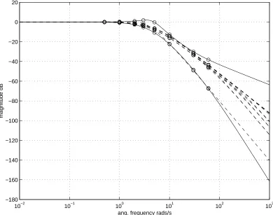
A second-order prefilter F(s) (of dc gain equal to 1 and cut-off frequencies 3.5 and 7.5 rads/s) was finally designed using the standard procedure [2]. Figure 4 shows the closed-loop frequency responses for a number of (a, k) parameter combinations, together with the tracking bounds|Bl(jω)| and |Bu(jω)|. Again, the eight frequencies of interest
are marked by circles. Clearly, the specifications of the design are met, as expected from the characteristics of the open loop response in Figure 3.
4
Conclusions
10−2 10−1 100 101 102 103 −180
−160 −140 −120 −100 −80 −60 −40 −20 0 20
ang. frequency rads/s
[image:12.612.93.483.79.386.2]magnitude dB
Figure 4: Closed-loop responses and bounds
be used to automate the loop-shaping step of the QFT design procedure. Although the algorithm has been presented for SISO systems, its extension to multivariable problems is possible using the standard QFT approach.
5
Acknowledgement
A. Zolotas would like to thank Mr Dimitriadis and Sevath ABE for providing him with the necessary computer equipment during the last phase of this work.
References
[1] BRYANT G.F. and HALIKIAS G.D., 1995, Optimal loop shaping for systems with large parameter uncertainty via linear programming. International Journal of Con-trol, 62, 557-568.
[2] D’AZZO, J. and HOUPIS C., 1998,Feedback Control Systems Analysis and Synthesis
(Prentice-Hall)
[4] HOROWITZ, I.M. and SIDI, M., 1972, Synthesis of feedback systems with large plant ignorance for prescribed time-domain tolerances. International Journal of Control,
16, 287-309.
[5] HOROWITZ, I.M. and SIDI, M., 1978, Optimum synthesis of non-minimum phase systems with plant uncertainty, International Journal of Control,27, 361-386.
[6] MACIEJOWSKI, J.M., 1989, Multivariable Feedback Design (Addison-Wesley).
[7] YANIV, O. and HOROWITZ, I.M., 1986, A Quantitative design method for MIMO linear feedback systems having uncertain plants. International Journal of Control,