Abstract—As a very recent technique for time series analysis, Singular Spectrum Analysis (SSA) has been applied in many diverse areas, where an original 1D signal can be decomposed into a sum of components including varying trends, oscillations and noise. Considering pixel based spectral profiles as 1D signals, in this paper, SSA has been applied in Hyperspectral Imaging (HSI) for effective feature extraction. By removing noisy components in extracting the features, the discriminating ability of the features has been much improved. Experiments show that this SSA approach supersedes the Empirical Mode Decomposition (EMD) technique from which our work was originally inspired, where improved results in effective data classification using Support Vector Machine (SVM) are also reported.
Index Terms—Singular Spectrum Analysis (SSA), Hyperspectral Imaging (HSI), feature extraction, data classification, Support Vector Machine (SVM).
I. INTRODUCTION
YPERSPECTRAL imaging (HSI) provides data with a high-resolution spectrum over 2D images, leading to powerful capabilities related to classification in many applications, such as remote sensing. The wide range covered by the spectral information, from visible light to near infrared, allows the recognition of small differential characteristics of the content in a scene. For that reason, new emerging lab-based data analysis including food quality, medical or verification of counterfeit goods and documents [1]-[4] are based on HSI. The use of Support Vector Machine (SVM) as a classifier for HSI applications has been shown to be robust and highly accurate [5]-[7]. The samples or pixels are evaluated in SVM by means of their respective features or spectral bands, which can contribute to more robust discrimination as they include information from different spectral wavelengths. However, HSI data usually is prone to noise, which can reduce the discrimination ability limiting the accuracy in classification tasks. For that reason, there is great interest for a potential decomposition of the spectral profiles into components in such a
Manuscript received November 25th, 2013; revised February 12th, 2014. Partial of the work was supported by National Science Foundation of China (61202165 and 61003201) and Royal Society of Edinburgh (6121130125).
J. Zabalza, J. Ren (corresponding author), and S. Marshall are all with Centre for excellence in Signal and Image Processing, Department of EEE, University of Strathclyde, Glasgow, U.K. (Emails: [email protected], [email protected], [email protected]).
Z. Wang is with School of Computer Software, Tianjin University, Tianjin, China (Email: [email protected]).
J. Wang is with School of Electronic and Information Engineering, Beijing Univ. of Aeronautics & Astronautics, China (Email: [email protected]).
way that noise could be removed or mitigated by avoiding particular components with high noisy content. In this decomposition context, a particularly interesting research area is the use of the Empirical Mode Decomposition (EMD) technique, applied in 1D to the spectral profile of the pixels as briefly evaluated in [8].
The EMD is the main part of the Hilbert Huang Transform (HHT), an algorithm for the analysis of non-linear and non-stationary time series [9]-[10]. EMD decomposes a 1D signal into a few components called Intrinsic Mode Functions (IMFs) and has been widely used in processing signal applications such as speech recognition [11]. The reconstruction of the 1D signal by some of their IMFs would provide an alternative signal that could be easier to classify. Although this was the objective, an evaluation in [8] showed no improvement at all but deterioration of classification accuracy.
Hence, our aim is to introduce the Singular Spectrum Analysis (SSA) technique in a similar way to evaluate its performance for classification tasks in HSI. In this paper, Section II describes SSA algorithm, its definitions and applications, and once our approach is clear, Section III outlines the experimental setup, with the results and analysis. Finally, the conclusions are given in Section IV.
II. THE PRINCIPLES OF SSA
SSA is a recent technique of time series analysis and forecasting with multiple potential in different applications, going from market research or social science to data mining. With origin in the former Soviet Union during the 80s, there are several related publications in the last twenty years, although some authors stand out [12]-[13]. In this section, the SSA concept and capabilities is briefly introduced, along with a complete mathematical description of the algorithm and a practical example for an easy understanding.
A. The Concept
The main objective of SSA is to decompose an original series into several independent components or sub-series. These components are interpretable, i.e. they can be mainly identified as varying trend, oscillations or noise. Therefore, the main capabilities of SSA can be summarized as follows [12].
- Extraction of trends, periodic components and smoothing
- Complex trends and periodicities with varying amplitudes
- Finding structures in short time series
- Envelopes of oscillating signals
Singular Spectrum Analysis for Effective
Feature Extraction in Hyperspectral Imaging
Jamie Zabalza, Jinchang Ren, Zheng Wang, Stephen Marshall, Jun Wang
All these capabilities make SSA a really interesting approach, especially as most researches have not yet taken it into consideration in HSI.
B. The Algorithm
Assume that we have a 1D signal in a vector arrayx defined
as N
N
x x
x [ 1, 2,, ]
x ; the SSA algorithm can be applied in the following steps.
i. Embedding
Defining a window size LZ satisfying L[1,N], the trajectory matrixXof the vector array x can be constructed as:
K
N L L K K x x x x x x x x x C C C
X 1, 2, ,
1 1 3 2 2 1
(1)
Each column of X,Ck, is a lagged vector which can be represented as Ck[xk,xk1,xkL1]TL , where
] , 1
[ K
k and KNL1. It is worth noting that the matrixXhas equal values along the anti-diagonals, thus it is actually a Hankel matrix by definition.
In fact, based on a property of the matrix X[12], the SSA algorithm can be implemented symmetrically in two intervals, i.e. L[1,round(N/2)] and L[ceil((N1)/2),N] . For a given L , the equivalent implementation can be found for anotherL'K, leading to the same results. In addition, just remark that both singular ends from the global interval, 1
andN, do not provide a SSA implementation.
ii. Singular Value Decomposition
First the matrix S is obtained from the trajectory matrix Xas SXXT . The Eigen values of S and their respective Eigen vectors are then denoted respectively as
1
2
L
and
U1,U2,,UL
.For the trajectory matrix X , its Singular Value Decomposition (SVD) is then formulated as given below. Though the value of d equals to the rank of X, from now on we considerdL for simplicity.
d
X X
X
X 1 2 (2) As can be seen, the trajectory matrixX is actually built by the addition of several matrices. Each matrix Xi|i[1,L] is called elementary matrix, corresponding to its respective Eigen value as defined by:
T i i i i UV
X (3) where Vi is defined as
i i T i U X
V (4)
Note that the collection
i,Ui,Vi
is normally called the ith Eigen Triple, and the matrices U and Vbelow are denoted as the matrix of empirical orthogonal functions and the matrix of the principal components, respectively.
K LL L L L V V V V U U U U 2 1 2
1 (5)
iii.Grouping
In this step, the total set of L components is divided into M disjoint sets I1,I2,,IM , where
|Im|L and] , 1 [ M
m . Let I
i1,i2,,ip
denote one of the divided set, the matrix XI related to the group I is defined asip i
i
I X X X
X 1 2 . Finally, the trajectory matrix X is represented by:
IM I
I X X
X
X 1 2 (6) For simplicity, a typical grouping is the one such asML, i.e.p1, which refers to the case that each set is made of just one component. In general, the contribution of each matrix XI to the trajectory matrix X in the SVD is related to its Eigen values and therefore can be derived as:
L i i I i i I 1 (7)
iv.Diagonal Averaging and Projection
The matrices XIm,m[1,M] obtained above by grouping are not necessarily the Hankel type as in the original trajectory matrix. However, in order to project each of these matrices into 1D signal, they have to be hankelised. This step is done by obtaining the average in all the anti-diagonals of eachXIm, simply because these values used for average contribute to the same element in the derived 1D vector array.
Let N
mN m
m
m[z 1,z 2,,z ]
z denote the 1D signal
projected fromXIm, it can be obtained via diagonal averaging below, where aj,nj1 refers to the elements of XIm.
N n K a n N K n L a L L n a n z L K n j j n j L j j n j n j j n j mn 1 1 , 1 1 , 1 1 , 1 1 1 1 1 (8)With zm obtained in (8), finally the original 1D signal x can be reconstructed by:
M m m M 1 21 z z z
z
As a result, the original signal can also be represented using one or more groups derived from its Eigen values, where those less significant components or highly noisy ones are discarded.
C. Application of SSA
Given a particular sample, e.g. a spectral pixel in HSI, the SSA aims to achieve improved reconstruction of the pixel profile by means of the main Eigen value components whilst abandoning the less representative or noisy components. For effective reconstruction of the original profile, there are two important parameters affecting the performance.
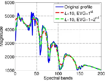
[image:3.612.315.564.60.215.2]The first parameter is the window size L, which determines the total number of components that can be extracted in the decomposition stage. Taking L=10 for example, ten Eigen values are extracted, which leads to ten potential components generated. Obviously, the component corresponding to the first Eigen value is much more significant than those corresponding to the following Eigen values.
Fig. 1. Original and reconstructed (by SSA) profiles for one pixel in HSI. The reconstructions are derived from the 1st and 1-2nd Eigen values out of 10.
The second parameter, Eigen Value Grouping (EVG), denotes the selected combination of extracted components used for reconstruction. For a dataset with highly noisy content, the use of only the first two components will remove most noise from the input data. However, if the noise level is low that only affects small components such as the 9th or the 10th, using just
the first two components in the reconstructed signal may lead to loss of discriminating information in the samples.
Fig. 1 shows an example where one spectral pixel is reconstructed from the 1st and 1-2nd Eigen components, using
L=10. As can be seen, the new profiles preserve the trend of the original signal whilst reducing the noisy content. As such, the feature extraction process by SSA results in better classification as will be further demonstrated in Section III.
III. EXPERIMENTAL RESULTS AND ANALYSIS
The experimental settings and results are discussed in detail below, covering data description and conditioning, feature extraction, data classification and relevant evaluations. All the experiments were implemented in the Matlab environment.
A. Data Description
Two remote sensing datasets with available ground truth are employed in our experiments. They consist of sub-scenes extracted from original scenes [14]-[15].
[image:3.612.315.565.250.402.2]Fig. 2. One band image at wavelength 667nm (left) and the ground truth maps (right) for the 92AV3C dataset.
Fig. 3. One band image at wavelength 667nm (left) and the ground truth maps (right) for the Salinas C dataset.
The AVIRIS 92AV3C dataset, collected in the USA, has a spatial dimension of 145×145 pixels in 220 spectral reflectance bands for land usage purpose. Although originally it contains 16 labeled classes, some authors suggest removing the classes with few pixels available in the ground truth [5], [7]-[8]. This has led to 9 out of 16 classes being included in the study for consistent evaluation. As shown in Fig. 2, the 9 labeled classes are mostly related to agriculture.
The AVIRIS Salinas C dataset (Fig. 3), a sub-scene taken over the Salinas Valley in California, USA, is made of 150×150 pixels in 224 spectral bands, with a spatial resolution of 3.7m. The ground truth map presents 9 classes corresponding to broccoli, fallow, grapes and vineyard amongst others.
It is worth noting that before feature extraction some spectral bands are discarded as recommended by others [7], [15], reducing the available number of bands from 220 to 200 and from 224 to 204 for the two datasets, respectively.
B. Feature Extraction
[image:3.612.81.256.266.402.2]TABLEI
DIFFERENT IMPLEMENTATIONS FOR FEATURE EXTRACTION
Method Parameters Values adopted
Baseline N/A N/A
EMD Thresholds θ1, θ2 and α 0.8, 8 and 0.05 IMF Grouping (IMFG) 1st, 1-2nd, 1-3rd
SSA Window size L 5, 10, 20, 40 EV Grouping (EVG) 1st, 1-2nd, 1-5th, 1-10th
In the Baseline approach, no feature extraction method is applied hence the original spectral profiles are used as features. As a result, no parameters are needed. For the EMD and SSA techniques, on the contrary, their performances are parameter dependent and the values used for them are given in Table I.
For the EMD case, where detailed algorithm description can be found in [9]-[11], the code available in [16] is used for its implementation with the stopping criteria discussed in [10]. The values adopted for the stopping thresholds θ1, θ2 and α are determined experimentally and satisfying θ2=10×θ1 as suggested. Regarding the IMF Grouping (IMFG) parameter, combinations of the 1st, the 1-2nd and the 1-3rd IMFs are
respectively selected in the same way as used in [8].
In the SSA case, as stated in Section II.C, performance depends on two parameters, window size L and EV Grouping (EVG). Several combinations of window size L (5, 10, 20 and 40) and EVG (the 1st, the 1-2nd, the 1-5th and the 1-10th) are
selected to evaluate the corresponding performance.
Finally, to provide further analysis on the comparison among the Baseline and SSA methods, well-known Principal Components Analysis (PCA) technique [2]-[3] is applied to the output of these cases for data reduction, adding an extra step.
C. Data Classification
SVM is selected as it has been widely used in HSI field [5]-[8]. With several available libraries, the difficulty in implementing SVM has been much reduced even for embedded applications [17]. For multi-class classification, LIBSVM library [18] is used in our experiments. A Gaussian RBF kernel is selected here as, from our own experience and also demonstrated by others [5]-[8], it usually leads to good results in HSI. For that kernel, the penalty (c) and the gamma (γ) parameters are tuned each time by means of a grid search.
To avoid systematic errors, 10 repetitions are carried out for every experiment, varying randomly each time the samples (sub-set) for training and testing. The partitions are made by stratified sampling, using an equal sample rate for each class with a ratio of 10% for training the respective SVM model. Finally, testing results averaged over 10 repetitions are obtained for performance evaluation, including McNemar’s test [8], which shows statistical significance at a confidence level of 95% when │Z│> 1.96, taking the Baseline case as a reference.
D. Results and Analysis
According to results in Table II, for the 92AV3C dataset, it is clear that the Baseline approach can be easily improved by SSA technique, which increases the discrimination ability. On the
other hand, the EMD technique is proved to decrease the accuracy, as already stated in [8]. For the Salinas C dataset, the SSA technique also improves the performance, although the classification accuracy of the Baseline approach is already very high (over 99%) and therefore Z coefficient is below 1.96 in some cases. Again, the EMD approach degrades the performance with the least classification accuracy produced, which indicates its unsuitability for effective feature extraction and data reduction in this context.
TABLEII
MEAN OVERALL ACCURACY (%) OVER TEN REPETITIONS AND MEAN
MCNEMAR’S TEST [Z] FOR THE TWO DATASETS AND THREE METHODS
Method Parameters 92AV3C Salinas C
Baseline N/A 85.59 [-] 98.61 [-]
EMD
IMFG=1st 56.44 [-44.1] 96.21 [-16.4] IMFG=1-2nd 65.52 [-33.8] 96.25 [-16.2] IMFG=1-3rd 75.49 [-20.1] 97.31 [-11.0]
SSA
L=5, EVG=1st 88.78 [+9.24] 98.76 [+2.03]
L=5, EVG=1-2nd 88.02 [+7.47] 98.69 [+1.21]
L=10, EVG=1st 88.68 [+8.87] 98.68 [+0.78]
L=10, EVG=1-2nd 88.49 [+8.57] 98.76 [+2.00] Other accuracy measures are shown in Table III for Baseline and SSA case (L=5, EVG=1st), proving the good performance
of SSA, where the increment in Average Accuracy is clear and in Class by Class terms, the improvement is generally obtained in all classes, regardless their number of samples.
TABLEIII
MEAN OVERALL,AVERAGE AND CLASS BY CLASS ACCURACIES (%) OVER TEN
REPETITIONS FOR THE TWO DATASETS WITH BASELINE AND SSA(L=5, EVG=1ST)METHODS,INCLUDING NUMBER OF SAMPLES (NOS)
92AV3C Salinas C
NoS Baseline SSA NoS Baseline SSA
Class 1 1434 80.71 84.81 240 95.32 95.56 Class 2 834 72.03 80.99 3400 99.93 99.92 Class 3 497 89.98 92.73 1957 99.71 99.80 Class 4 747 97.23 97.77 599 99.13 98.42 Class 5 489 99.00 99.11 1155 97.77 98.40 Class 6 968 76.83 83.54 1414 99.99 99.99 Class 7 2468 83.99 86.11 848 99.62 99.65 Class 8 614 80.45 84.91 5890 99.23 99.35 Class 9 1294 98.27 98.41 159 25.52 32.59 Average Accuracy 86.50 89.82 90.69 91.52 Overall Accuracy 85.59 88.78 98.61 98.76
In fact, these three regions, noisy, lossy and stable, can be clearly identified in Fig. 4, such as noisy (L=10, EVG=1-5th),
lossy (L=40, EVG=1st) and stable (L=5, EVG=1st). When the
window size increases from 5 to 40, EVG=1st tendency is going
[image:5.612.53.293.483.553.2]from stable to lossy region, whilst EVG=1-10th is going from noisy to stable. Finally, please note that some points (L=5, EVG=1-5th) and (L=10, EVG=1-10th) are equivalent to each other, simply because the reconstruction is made by all the components extracted from the decomposition.
Fig. 4. Overall Accuracy (%) for the 92AV3C dataset using SSA with different window L (5, 10, 20 and 40) and different EVG (1st, 1-2nd, 1-5th and 1-10th).
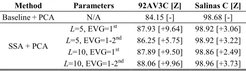
Finally, extra results are provided in Table IV for a more complete evaluation. PCA is applied to both Baseline and SSA outputs, reducing the number of features to 15. As expected, these results again confirm that SSA leads to considerable improvement under different conditions, especially for the 92AV3C dataset, even in combination with PCA. However, due to a low feature dimension used, the classification accuracy achieved appears slightly worse than those in Table II.
TABLEIV
MEAN OVERALL ACCURACY (%) OVER TEN REPETITIONS INCLUDING MEAN
MCNEMAR’S TEST [Z] OF BASELINE AND SSA WITH PCA(15FEATURES)
Method Parameters 92AV3C [Z] Salinas C [Z]
Baseline + PCA N/A 84.15 [-] 98.68 [-]
SSA + PCA
L=5, EVG=1st 87.93 [+9.64] 98.92 [+3.06]
L=5, EVG=1-2nd 86.25 [+5.75] 98.92 [+3.22]
L=10, EVG=1st 87.89 [+9.50] 98.86 [+2.49]
L=10, EVG=1-2nd 88.06 [+9.96] 98.96 [+3.73]
IV. CONCLUSIONS
As a recent technique being able to extract trends, oscillatory components or noise among others from 1D signal, the SSA algorithm shows great potential in many applications. Components extracted from the decomposed signal can be used for an improved reconstruction of the original signal with noise information suppressed.
Inspired by the EMD algorithm, and based on the well-known Eigen decomposition, SSA allows many possibilities and presents significant potential. In HSI remote sensing, the introduction of the SSA applied to every spectral pixel leads to a reconstruction process that increases the accuracy in classification tasks, as derived in the experimental results from
our work. Some introductory evaluation about the behavior of the SSA approach when implemented by different parameters selection is reported, by which it is possible to state recommendations for the selection of parameters. Future work is ongoing in extending 1D SSA to 2D cases for further improved feature extraction and data reduction in HSI applications.
REFERENCES
[1] V. E. Brando and A. G. Dekker, “Satellite hyperspectral remote sensing for estimating estuarine and coastal water quality,” IEEE Trans. Geoscience and Remote Sensing, vol. 41, pp. 1378-87, 2003.
[2] J. Ren, S. Marshall, C. Craigie and C. Maltin, “Quantitative assessment of beef quality with hyperspectral imaging using machine learning techniques,” 3rd Int. Conf. Hyperspectral Imaging, 2012.
[3] K. Gill, J. Ren, et al, “Quality-assured fingerprint image enhancement and extraction using hyperspectral imaging,” 4th Int. Conf. Imaging for Crime
Detection and Prevention, 2011.
[4] T. Nagaoka, A. Nakamura, Y. Kiyohara, T. Sota, “Melanoma screening system using hyperspectral imager attached to imaging fiberscope,”
Engineering in Medicine and Biology Society, pp. 3728-3731, 2012. [5] F. Melgani and L. Bruzzone, “Classification of hyperspectral remote
sensing images with support vector machines,” IEEE Trans. Geoscience and Remote Sensing, vol. 42, no. 8, pp. 1778-1790, Aug. 2004. [6] M. Pal and G. M. Foody, “Feature Selection for Classification of
Hyperspectral Data by SVM,” IEEE Trans. Geoscience and Remote Sensing, vol. 48, no. 5, May 2010.
[7] R. Archibald and G. Fann. “Feature Selection and Classification of Hyperspectral Images with Support Vector Machines.” IEEE Geoscience and Remote Sensing Letters, vol. 4, no. 4, October 2007.
[8] B. Demir and S. Ertürk, “Empirical mode decomposition of hyperspectral images for support vector machine classification,” IEEE Trans. Geoscience and Remote Sensing, vol. 48, no.11, pp. 4071-4084, 2010. [9] N. E. Huang et al, “The empirical mode decomposition and the Hilbert
spectrum for nonlinear and non-stationary time series analysis”,
Proceedings of the Royal Society A, Math. Phys. Sci., vol. 454, no. 1971, pp. 903-995, Mar. 1998.
[10] G. Rilling, P. Flandrin, and P. Gonçalvés. “On empirical mode decomposition and its algorithms.” IEEE-EURASIP Workshop on Nonlinear Signal and Image Processing NSIP. vol. 3. 2003.
[11] H. Huang and J. Pan, “Speech pitch determination based on Hilbert-Huang transform,” Signal Processing, vol. 86, no. 4, 2006. [12] N. Golyandina and A. Zhigljavsky, Singular Spectrum Analysis for Time
Series, Springer, 2013.
[13] N. Golyandina, V. Nekrutkin, and A. A. Zhigljavsky. Analysis of time series structure: SSA and related techniques. Chapman-Hall/CRC, 2001. [14] Pursue's university multispec site: June 12, 1992 aviris image Indian Pine
Test Site [Online]. Available:
https://engineering.purdue.edu/~biehl/MultiSpec/hyperspectral.html [15] Hyperspectral Remote Sensing Scenes [Online]. Available:
http://www.ehu.es/ccwintco/index.php/Hyperspectral_Remote_Sensing_ Scenes
[16] A. Linderhed. Image Empirical Mode Decomposition Matlab Code [Online]. Available: http://aquador.vovve.net/IEMD/
[17] J. Zabalza, J. Ren, C. Clemente, G. Di Caterina, and J. J. Soraghan, “Embedded SVM on TMS320C6713 for Signal Prediction in Classification and Regression Applications,” in 5th European DSP Education and Research Conf., Amsterdam, Sept. 2012.