1
Object Detection in Optical Remote Sensing Images Based on Weakly
Supervised Learning and High-level Feature Learning
Junwei Han
1, Dingwen Zhang
1, Gong Cheng
1, Lei Guo
1, and Jinchang Ren
2 1School of Automation, Northwestern Polytechnical University, Xi’an, 710072, China
2
Department of Electronic and Electrical Engineering, University of Strathclyde, UK
Abstract
The advance of remote sensing technology has been capable of providing abundant spatial and contextual information for object detection in optical satellite or aerial imagery, which facilitates subsequent automatic analysis and interpretation of the optical remotes sensing images (RSIs). Most existing object detection approaches suffer from two limitations. First, the feature representation used is insufficiently powerful to capture the spatial and structural patterns of objects and the background regions. Second, a large number of training data with manual annotation of object bounding boxes is required in the supervised learning techniques adopted while the annotation process is generally too expensive and sometimes even unreliable. To tackle these two limitations, a novel and effective geospatial object detection framework is proposed by combining the weakly supervised learning (WSL) and high-level feature learning. First, we employ an unsupervised feature learning approach via Deep Boltzmann Machine (DBM) to infer the spatial and structural information encoded in the low-level and middle-level features, which facilitates good semantic preserving ability for effective describing objects in optical RSIs. Then, we present a novel WSL approach to object detection in optical RSIs where the training sets require only binary labels indicating whether an image contains the target object or not. Based on the learnt high-level features, it jointly integrates saliency, intra-class compactness, and inter-class separability in a Bayesian framework to initialize a set of training examples from weakly labeled images and start iterative learning of the object detector. A novel evaluation criterion is also developed to detect model drift and cease the iterative learning. Comprehensive experiments on three optical RSI datasets with large variations in terms of spatial resolution, and types of objects have demonstrated the efficacy of the proposed approach in benchmarking with several state-of-the-art supervised learning based object detection approaches.
Keywords:
Weakly supervised learning,Bayesian framework, Object detection, Unsupervised feature learning, Deep Boltzmann Machine.1.
Introduction
2
objects contained in optical RSIs has offered us the new opportunity to address this challenging task. Early attempts [1, 4, 5] detected objects in optical RSIs in an unsupervised manner which often started from generating region of interest (ROI) by grouping pixels into clusters and then detected objects of interest based on the shape and spectral information. Afterward, many supervised learning methods have been adopted to learn the object model effectively with the help of prior information obtained from training examples [2, 6-8]. By heavily relying on the human labelled training examples which are statistically representatives of the classification problem to solve, the supervised learning methods can achieve more promising performance than the unsupervised approaches. Therefore, overwhelming object detection systems are usually based on the supervised learning techniques.
The recent advance of remote sensing technology has led to the explosive growth of satellite and aerial images in both quantity and quality. It brings about two increasingly serious problems for the object detection task in optical RSIs. First, supervised learning based object detection approaches often require a large number of training data with manual annotation of labeling a bounding box around each object to be detected. However, manual annotation of objects in large image sets is generally expensive and sometimes even unreliable. For example, for the natural objects such as landslide, the proper manual annotation generally requires considerable expertise. In addition, manual annotation is also difficult for the man-made objects such as airplane and car, where the coverage of target object appears to be very small, especially when complex textures are contained in the image background. As a result, it is difficult to achieve accurate annotation on such small regions. Moreover, the manual annotations may tend to be less accurate and unreliable when the targets are occluded or camouflaged. As a result, it is a great interest in training object detectors with weak supervision for large-scale optical satellite and aerial image datasets.
The second problem is that the rich information contained in the optical RSIs with high spatial resolution has more details of objects whereas feature descriptors used by existing object detectors are still insufficiently powerful to characterize the structural information of the objects. The limited understanding of the spatial and structural patterns of objects in optical RSIs leads to a tremendous semantic gap for the object detection task. It can be observed that man-made facilities, such as airplanes, vehicles and airports, always have intrinsic structural property with specific semantic concepts, which has obvious difference from the background areas in optical RSIs. Consequently, building of the high-level structural and semantic features is a promising way for the interpretation of the optical RSIs and object detection task.
3
results and thus we can obtain final object detector with satisfactory performance.
To tackle the problem of insufficiently powerful feature descriptors, we explore the spatial and structural information within image patches via high-level feature learning. Unlike existing works to extract structural features solely based on human design [9, 10], the proposed approach derives high-level features by applying unsupervised representation learning approach, where spatial and structural patterns from the low-level and middle-level features can be automatically captured. Here we adopt Deep Boltzmann Machines (DBM) to learn high-level feature because it has been demonstrated to have the potential of learning useful distributed feature representations and become a promising way in solving object and speech recognition problems [11-13].
In summary, the main contributions of this paper are threefold.
1) We propose a novel WSL framework based on Bayesian principles for detecting objects from optical RSIs, which extensively reduces human labors for annotating training data while achieving performance comparable to that of the fully supervised learning approaches;
2) We propose unsupervised feature learning via DBM to build high-level feature representation for various geospatial objects. The learned high-level features capture the structural and spatial patterns of objects in an effective and robust fashion, which leads to further improvement of object detection performance;
3) Extensive evaluations on three optical RSI datasets with different spatial resolutions and objects of interest are carried out to validate the effectiveness of the proposed methodology. The rest of the paper is organized as follows. Section 2 gives a brief review of the related work. Section 3 introduces the proposed framework. Section 4 proposes the unsupervised feature learning. Section 5 describes the WSL framework for object detection in optical RSIs. Experimental results are presented in Section 6. Finally, conclusions are drawn in Section 7.
2.
Related Work
Object or target detection in optical RSIs has been extensively studied in the past decades. For example, Li et al. [4] developed an algorithm for straight road edge detection from optical RSIs based on the ridgelet transform with the revised parallel-beam Radon transform. Ge at el. [5] detected inshore ships in optical satellite images by using shape and context information that are extracted in the segmented image. Liu et al. [1] presented robust automatic vehicle detection in QuickBird satellite images by applying morphological filters for road line removing and histogram representation for separating vehicle targets from background. All these methods are performed in an unsupervised manner. They are effective for detecting the designed object category in simple scenario.
4
A few efforts [14-17] have been performed to alleviate the work of human annotation. One interesting idea is to adopt semi-supervised learning model. Such methods apply a self-learning or active learning scheme where machine learning algorithms can automatically pick the most informative unlabeled examples based on a limited set of available labeled examples. Then, these picked unlabeled examples are combined with the initial labeled examples for the training of object detector or classifier. Specifically, Liao et al. [16] proposed a semi-supervised local discriminant analysis method for feature extraction in hypespectral RSI. Dópido et al. [15] adapted active learning methods to semi-supervised learning for hyperspectral image classification. Jun et al. [18] presented a semi-supervised spatially adaptive mixture model to identify land covers from hyperspectral images.
Although semi-supervised learning methods can considerably reduce the labor of human annotation, they still inevitably require a number of precise and concrete labeled training examples where each object is manually labeled by a bounding box in positive training images. WSL is desirable to further reduce the human labor significantly, where the training set needs only binary labels indicating whether an image contains the object of interest. Although a few WSL approaches have been applied to natural scene image analysis [19-22], those existing methods cannot be directly used to the field of RSI analysis as they have insufficient capability to handle the challenges in RSIs which contain large-scale complex background and a number of target objects with arbitrary orientation. As an initial effort, in our previous work in Zhang et al. [23], WSL was adopted and heuristically combined with saliency-based self-adaptive segmentation, negative mining algorithm, and negative evaluation mechanism for target detection in RSIs. Although it introduced some new concepts for WSL based target detection, the work lacks a principled framework and ignores some important information, which thus can be largely improved. In this paper, we propose a novel principled WSL framework for detecting targets from RSIs. Compared with [23], our improvements in this paper lie in threefold: 1) we propose a powerful high-level feature learning using DBM; 2) we propose a probabilistic approach via the Bayesian rule to jointly integrate saliency, intra-class compactness, and inter-class separability to initialize the training examples; and 3) we propose a novel scheme for model drift detection using the information from both negative training images and positive training images. The experimental results reported in subsection 6.4 can fully demonstrate these improvements.
3.
Overview of the Proposed Method
Given a training optical RSI set with weak label only indicating whether a certain category of object is contained in an image or not, the objective of the proposed work is to detect target objects of the same class within the testing images. Because these images generally have very large scale and contain multiple objects of interest, a straightforward way of processing is to decompose the images into small patches by sliding windows, and then predict whether each patch contains the object of interest. As suggested in [2, 3, 14], we adopt the multi-scale sliding window mechanism to handle the variational size of target objects.
The proposed object detection framework consists of two major components: unsupervised feature learning and WSL based object detection. The flowchart of the feature learning component (Section 4)
5
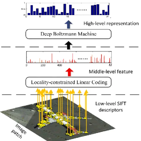
Fig. 1. High-level feature representation of the image patch.
Based on the obtained high-level features, the component of WSL based object detection shown in Fig. 2 (Section 5) contains two stages: training and testing. The objective of the training stage is to learn an object detector. In the testing stage, the learned object detector is applied to detect objects in a given testing image. The training stage includes two major steps: training example initialization (Subsection 5.1) and iterative object detector training (Subsection 5.2). For the first step, a Bayesian approach is proposed to integrate three kinds of important information of saliency, intra-class compactness, and inter-class separability, which estimates the probability of an image patch being the object of interest. After initializing the training examples, we are inspired by the bootstrapping method
[24] to train the object detector in an iterative process. In each iteration, the detector is utilized as an
annotator to refine the positive training set, which is then used to re-train the object detector. Thus both the training examples and object detector could be gradually updated to be more precise and strong. Afterwards, a novel detector evaluation method is proposed to detect the model drift and stop the iterative process automatically for obtaining the final object detector.
[image:5.595.50.551.571.743.2]6
4.
High-level Feature Representation
Feature description plays an important role in the task of object detection in optical RSIs. However, the performance of the existing feature descriptions in RSI analysis is still far from satisfactory. The main issue lies in the insufficiency in extracting features using only the pixel-based spectral information, which ignores the contextual spatial information and thus fails to capture the more important structural pattern of the object. With the advance of the remote sensing technology, optical satellite and aerial imagery with high spatial resolution makes capturing spatial and structural information possible. Nowadays, accurate interpretation of optical RSI relies on effective spatial feature representation to capture the most structural and informative property of the regions in each image. A number of such approaches have started to explore the spatial information by applying some low-level descriptors (such as SIFT, HOG and GLCM in [6, 25, 26]) or middle-level features (such as BOW and PLSA in [2, 26]) to represent image patches. Although to some extent these human designed features can improve the classification and detection accuracies in optical RSIs, they still suffer from several problems. Specifically, these low-level descriptors only catch limited local spatial geometric characteristics, which cannot be directly used to describe the structural contents of image patches. The middle-level features are usually extracted based on the statistic property of the low-level descriptors in an image patch to capture the structural information of the spatial region. However, it cannot provide enough strong description and generalization ability for object detection in complex backgrounds.
To tackle these problems, we build high-level feature representation via DBM to capture the spatial and structural patterns encoded in the low-level and middle-level features. DBM is one type of neural networks with deep architecture that learns feature representation in an unsupervised manner and has been demonstrated to be promising for building high-level feature descriptors [11, 12]. We therefore use it to map the middle-level features to the high-level representation that is highly accurate in characterizing different scenes or objects in optical RSIs. Specifically, the extraction of high-level feature representation (shown in Fig. 1) is carried out in three main stages: (1) Low-level feature descriptor extraction: a collection of low-level local descriptors are calculated by using scale-invariant feature transform (SIFT) [27]. (2) Middle-level feature generation: low-level descriptor of each image patch is coded by Locality-constrained Linear Coding (LLC) model [28]. (3) High-level feature learning: DBM [13] is adopted to learn more powerful representation from the middle-level feature.
4.1 Low-level descriptor extraction
We use low-level features to characterize the local region of each key point in image patches. Due to its ability to handle variations in terms of intensity, rotation, scale, and affine projection, the SIFT descriptor [27] is adopted in the proposed algorithm as the low-level descriptor to detect and describe the key points. According to existing work [2, 14, 29], the SIFT descriptor has been demonstrated to outperform a set of existing descriptors and widely used in analyzing RSIs.
4.2 Middle-level feature generation
To alleviate the unrecoverable loss of discriminative information, we apply the Locality-constrained Linear Coding (LLC) model [28] to encode the local descriptors into image patch representation. Specifically, all the extracted low-level descriptors are first clustered to generate a
codebook by using the K-means method. Let D[ , , ,d d1 2 dN] denotes a set of N extracted
7
LLC converts each descriptor into a M -dimensional code to generate the final image representation by
the following three steps. 1) For each input low-level descriptor dn, n[1, ]N , its five nearest
neighbors in CB are used as the local bases LBn, n[1, ]N to form a local coordinate system [28];
2) The local code cn is obtained by solving an objective function
2
1 1
|| || . 1
min N dn c LBn n N cn
n n
st
(1)Then the full code cn is generated, which is an M1 vector with five non-zero elements whose values correspond to cn. 3) The final middle-level image patch representation is yielded by max pooling
all the generated codes within the patch.
4.3 High-level feature learning
A DBM [13] is a neural network with deep structure constructed by stacking multiple Restrict Boltzmann Machine (RBM). In our framework, a three-layered DBM is adopted to capture structural and spatial patterns from middle-level features and learn high-level representations in an unsupervised
manner. It contains a visible layer v{0,1}M
and two layers of hidden units h1{0,1}H1, h2{0,1}H2.
Here, H1 and H2 indicate the numbers of units of the first hidden layer and the second hidden layer,
respectively. The energy of the state { , , }v h h1 2 is defined as
1 2 T 1 1 1T 2 2
( , , ; )v h h v W h h W h
E (2)
where {W W1, 2} are the model parameters, representing visible-to-hidden and hidden-to-hidden
symmetric interaction terms. The probability that the model assigns to a visible vector v is given by the Boltzmann distribution:
1 2
1 2
, 1
Pr( ; ) exp( ( , , ; ))
( )h h
v E v h h
Z
(3)where 1 2
1 2 ,
( )= v h h exp( ( , , ; ))v h h
Z
E is the partition function.The conditional distributions over the visible units and the two sets of hidden units are given by:
2
1 2 1 2 2
1 1
Pr( 1| , ) ( )
= =
v h
H M
i mi m ij m
m j
h sigm
W v
W h (4)1
2 1 2 1
1 Pr( j 1| )h (H mj i)
i
h sigm W h
8
1
1 1 1
1
Pr( 1| )h ( )
H
m mi i
i
v sigm W h
(6)where sigm( ) is a sigmoid function.
Given a set of training data, learning of DBM is a process to determine the related model
parameters {W W1, 2} in Eq. (2). Although exact maximum likelihood estimation of these
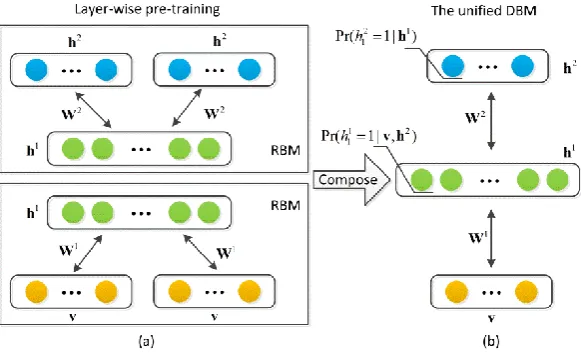
[image:8.595.152.443.291.470.2]parameters is intractable, efficient approximate learning of DBMs can be carried out by using mean-field inference together with the Markov Chain Monte Carlo algorithms [13]. Furthermore, the entire model can be efficiently pre-trained in a greedy layer-by-layer unsupervised manner by minimizing the energy function in each individual RBM model (shown in Fig. 3 (a)). Composing the RBM models afterwards forms a unified DBM model (shown in Fig. 3 (b)), which can be used to extract high-level feature representation.
Fig. 3. Learning processes for DBM.
In the proposed algorithm, all the middle-level features extracted from the image patches in training images are used as the input data to train DBM where the second hidden layer is used to build the final high-level feature representation for each image patch.
5.
WSL based Object Detection
5.1 Training example initialization
By applying sliding windows as pre-processing, the training images are divided into many patches.
Thus, the patch-level training data X+={ | x pp [1, ]}P and X={ | x qq [1, ]}Q can be generated from
the positive training images and negative training images, respectively. Our first task is to select
potential target object patches from X+ to generate the initial positive training set + 0
X . Typically,
9
of foreground objects. The intra-class compactness enforces the selected positive examples to be visually similar to each other, whilst the inter-class separability ensures that all selected positive examples are different from negative examples. In this paper, a novel Bayesian framework is proposed to combine these three types of information simultaneously to initialize the positive example training set as follows.
Let a binary random variable yp denote whether or not an image patch xp belongs to one
specified object. According to Bayes’ rule:
Pr( | 1) Pr( 1) Pr( 1| )
Pr( )
p p p
p p
p
x y y
y x x
(7)
Pr( | 0) Pr( 0)
Pr( 1| ) 1 Pr( 0 | ) 1
Pr( )
p p p
p p p p
p
x y y
y x y x
x
(8)
After adding the above two equations and omitting the constant term, we have
(9)
In the information theory, log Pr( )xp
, which is the log form of 1 Pr( )xp
, is known as the
self-information of the random variable xp [7, 30]. Self-information increases when the probability of
a patch decreases. In other words, patches that are discriminative from surrounds are more informative
and thus more likely to be the foreground object. Therefore, the term of 1 Pr( )xp
in Eq. (9) is
associated with the saliency information. The term Pr( |x yp p 1) indicates the likelihood that favors
image patches sharing the similar characteristic with the class of objects of interest. Hence it can be
considered as the metric of intra-class compactness. Similarly, the term Pr( |x yp p 0)
reflects the
distinctness of image patches in positive images and negative images, thus it corresponds to the metric
of inter-class separability. Finally, the remaining two prior probabilities Pr(yp 1) and Pr(yp 0) are
treated as the weights of intra-class metric and inter-class metric, respectively.
5.1.1 Saliency
As we assume that objects to be detected are normally one kind of foreground objects, our objective then becomes to quantify how likely each image patch is a foreground object. Foreground objects are generally informative and salient from the surrounding background as shown in Fig. 4. In computer vision, saliency detection technique can be used to estimate the saliency for each image patch. In recent years, it is also employed for the analysis in the domain of remote sensing [31, 32]. Inspired by [31, 33], we adopt sparse coding theory to calculate saliency based on the raw pixels to reveal the structural difference between an image patch and its surrounding. For each image patch xp (the patch
10 patches (patches indicated by green frames in Fig. 4) by:
χp Dicpαp (10)
where χp is the raw pixels within xp, while Dic
p and αp indicate the dictionary constructed by all
[image:10.595.206.388.158.376.2]surrounding patches and the sparse codes, respectively.
Fig. 4. An illustration of saliency calculation.
The rationale behind Eq. (10) is to represent χp approximately by its surrounding patches.
According to [31, 33], the coding sparseness ||αp||0 and the coding residual r =p χpDicpαp indicates
the saliency of the image patch xp with respect to its surrounding. Therefore, we estimate the saliency
by:
0 1
1 Pr( )xp =||αp|| ||r || p
(11)
5.1.2 Intra-class compactness
The intra-class compactness metric termed as Pr( |x yp p 1) in our framework aims to constrain
the similarity between positive examples. As positive examples of a specific object category should be visually similar, we can use a Gaussian Mixture Model (GMM) to estimate the probability distribution
of all positive examples. Then, Pr( |x yp p 1) measures how likely each image patch is a positive
example. Image patches with large Pr( |x yp p 1)
may be selected as positive examples. We use the
high-level feature fp (described in Section 4) to represent each image patch xp as this feature can
handle the variations in scale and orientation and capture the spatial and structural patterns of each image patch. As patterns learned using DBM are approximately independent, the joint probability is
11 2
1
Pr( | 1)= Pr([ ] |f 1)
H
p p p j p
j
x y y
(12)where [ ]fp j indicates the j-th dimensional value of fp and H2 indicates the dimensionality of
fp
as defined in Section 4. The distribution of each hidden unit’s response is estimated using GMM
with adaptive component K+j1, H2 by:
2
1
Pr([ ] |f 1)= j + ([ ] |f +, +)
K
p j p jk p j jk jk
k
y N
(13)where
+jk,
+jk,
2jk+ are parameters of the GMM in the k-th component for the j-th dimensionalfeature. All parameters are inferred based on object candidates in X+ by using the
expectation-maximization (EM) algorithm and Bayesian inference [34]. Here, X+ denotes the set of
object candidates and will be described in subsection 5.1.5.
5.1.3 Inter-class separability
Inter-class separability metric is to enforce the selected positive examples are dissimilar to negative examples. In WSL, the most confident information comes from the negative training images because they definitely do not contain the target. It is also reasonable to believe that the positive examples containing target objects should be different from the negative image patches in the negative images. Consequently, we can collect a large number of negative image patches to estimate the probability distribution of negative examples via a GMM. Then, we formulate the inter-class metric as the
likelihood term Pr( |x yp p 0), which reflects the probability of a certain image patch appearing in
negative training images. The high probability of the appearance in negative images would lead to low
inter-class difference and separability. Similar to Pr( |x yp p 1), Pr( |x yp p 0) can be decided based
on the high-level feature by:
2
1
Pr( | 0)= Pr([ ] |f 0)
H
p p p j p
j
x y y
(14)2
1
Pr([ ] |f 0)= ([ ] |f , )
j
K
p j p jk p j jk jk
k
y N
(15)where parameters
jk
,
jk
,
2jk
and Kj
are inferred by GMM based on all the negative image
12
5.1.4 Prior probability
Pr(yp1) and Pr(yp 0) are two prior terms in the proposed Bayesian framework. According to
[34], Bayesian methods would result in poor performance when inappropriate choices of prior are applied without any prior belief. Therefore, inspired by [35] we define the prior terms to reflect the
prior belief. Our prior belief is that Pr(yp 0) should be high when the content of certain image patch
p
x has small distance to the negative image patches in X, and Pr(yp1) should become high
when the content of xp
is close to the object candidates in X . Hence, we simply adopt the +
Nearest-Neighbor (NN) distance [36] to estimate these prior probabilities as:
1
Pr(yp 0) exp{= ||xpNn( ) }xp || (16)
1
Pr(yp 1) exp{= ||xpNp( ) }xp || (17)
where ||||1 is the L1 norm. Same as in [21, 36], Nn( )xp and Np( )xp refer to the nearest-neighbor
of xp in X and X+ (in terms of the high-level feature described in Section 4), respectively.
Finally, these two prior terms are used as the weights of the inter-class and intra-class metrics in order to reflect the prior probability that an image patch belongs to the positive and negative training
example, respectively.
5.1.5 Implementation details
In terms of Eq. (9), the post probability Pr(yp 1|xp) are estimated by integrating the saliency,
intra-class and inter-class metrics. Note that before calculating the intra-class compactness metric, X+
needs to be available. The work [22] proposed an exhaustive searching strategy to generate one object candidate for each image. However, it is lack of accuracy and efficiency for the large-scale RSIs especially when it contains multiple target objects locating at quite scattered positions. To tackle this challenging problem, we in practice implement our work in two stages.
In the first stage, we calculate the post probability Pr(yp 1| )xp approximately by only using the
saliency and inter-class separability metrics to generate X+ . As initially Pr( | 1) p p x y
and
Pr(yp 0) are unknown, we omit them by following [7, 30], which is equivalent to assuming a
uniform likelihood distribution for the unspecified object category. The overall formulation reduces to: 1
Pr( 1| ) [1 Pr( | 0) Pr( 0)]
Pr( )
p p p p p
p
y x x y y
x
(18)
13
+={ | Pr( 1| ) }
p p p
X x y x (19)
Once X+ is obtained, we fully implement the proposed Bayesian framework in the second stage,
where all the three types of information are explored and integrated for calculating Pr(yp 1|xp) by
Eq. (9). Similar to the first stage, a threshold is chosen to determine the label of each image patch
and thus generate the initial positive training set + 0
X by:
+
0 ={ | Pr(p p 1| p) }
X x y x (20)
By considering the fact that imbalanced positive and negative training data may reduce the performance of the object detector, we follow the previous work of [24] to generate the initial negative
training set X0 by randomly under-sampling of X to the same size as + 0
X . Some examples in the
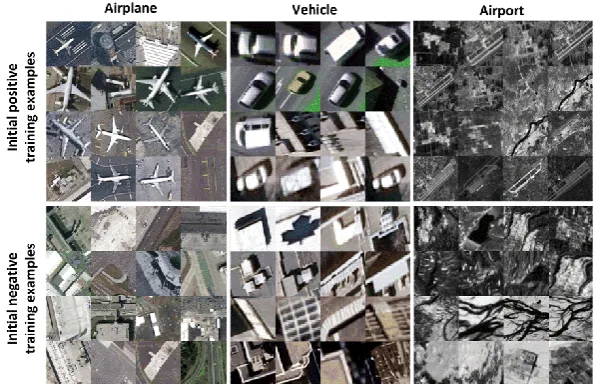
[image:13.595.149.448.321.513.2]initial training set are shown in Fig. 5.
Fig. 5. Some examples in initial positive and negative training set.
5.2 Iterative detector training
After obtaining the initial training examples, the object detector is trained iteratively in the proposed framework (shown in Fig. 2). In each iteration, the training set generated by the previous iteration is used to train the current object detector, which in turn updates the training examples for the next iteration. The iteration process stops when a model drift is detected by a novel detector evaluation method. Then the object detector obtained before model drift is regarded as the final object detector.
5.2.1 Training example and object detector update
14
SVM formulation, we use the below score function for object annotation and detection.
1 1
( )p w fp
Score x b (21)
where the variables w1 and b1 are defined as the SVM decision plane and its bias, which are learnt
from the initial training data. With the score function, binary class label yp are assigned to the image
patch xp based on the sign of the function.
1 ( ) 0
0 ( ) 0
= p
p
p
S c o r e x y
S c o r e x ,
, (22)
In order to obtain more precise object patches as the updated positive training examples, an adaptive threshold is used to determine image patches that have higher confidence to be the object of interest.
1
1 1
{ | p ( )p P p ( )p P p}
p p
X x Score x y Score x y
(23)where X1 is the updated positive training set after the first iteration. Afterwards, the same number of
negative examples randomly selected from X are used to generate the new negative training set X1
.
Alternating the update of object detector and training examples progressively improve their accuracy until the end of the iteration. Combination of these two stages in an iterative way is very similar to the bootstrapping [24] or active learning [14] strategy, which allows the proposed WSL based object detection in optical RSIs to achieve good performance that even superior than the traditional supervised learning methods in some cases.
5.2.2 Detector evaluation
Similar to the model drift phenomenon in adaptive object tracking, the performance of the trained object detector is improved in the first several iterations, continually, and then begins to degrade. Consequently, generating reasonable evaluation mechanism to detect the model drift is important. As the exact location of the objects of interest in each positive training image is unknown, thus it is impossible to measure directly whether a stronger object detector has been obtained after each iteration. It brings great challenge for evaluating the object model and detecting model drift in WSL.
Firstly we use a negative example based evaluation mechanism to estimate the performance of the trained object detector in each iteration. In general, a good object detector is expected to obtain detection results with high true positives and low false positives. In the WSL, we can only obtain precise negative image patches which certainly contain no object of interest. As a result, the negative evaluation mechanism is adopted here to approximately evaluate the false positive rate for the object detector. Specifically, for each iteration, the trained object detector is applied to classify each image patch with the negative training images and then calculate the false positive rate FR by:
| false| / | | FR X X
(24)
{ | ( ) 0}
false q q
X x Score x
15
where fq refers to high-level features of xqX and | | denotes the number of elements.
Another evaluation mechanism is based on the estimation of the object detector’s performance in
positive training images. Here we define GMM+ and GMM as the distributions inferred by GMM
based on the positive and negative examples, respectively. As the positive training examples are updated
after each iteration, the distribution of the j-th dimensional high-level feature is modified along the
iteration as: 2 1 ( +, +) = j K
j jk jk jk
k
GMM N
(26)where
jk,
jk,
2jk and Kj are inferred based on the updated positive training examples aftereach iteration. In contrast, GMM is fixed as:
2 1 ( , ) = j K
j jk jk jk
k
GMM N
(27)where
jk
,
jk
,
2jk
and Kj
are inferred based on the constant negative image patches in X. In
the first iteration, the object detector trained on the initial training examples is not very accurate. Thus the trained object detector may work unsatisfiedly and the updated positive examples generate the
+
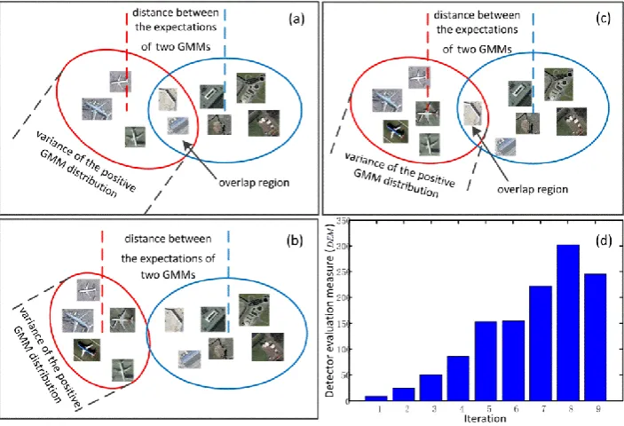
GMM distribution having amount of overlap with the GMM distribution as shown in Fig. 6 (a).
After several iterations, if the object detector is getting stronger, the overlap between the two distributions should become less as shown in Fig. 6 (b). Finally, when the detector starts to drift towards some noise patches without containing objects of interest, the overlap tends to large again as shown in Fig. 6 (c). Consequently, we evaluate the object detector and monitor the model drift by estimating the
overlap between the two GMM distributions in each iteration. As the GMM distribution is fixed, the
distance between the expectations of the two distributions and the variance of GMM+ distribution are
used to approximately predict the overlap area. Intuitively, the GMM+ distribution with expectation
away from that of GMM and small variance has small overlap with the distribution of the GMM
and vice versa (shown in Fig. 6). According to [34], the expectation andvariance of the GMM+ for the
-th
j dimensional high-level feature are decided by:
1
x( ) j
K
j jk jk
k
GMM
16
2 2 2
1
Var( ) ( ) x( )
j
K
j jk jk jk j
k
GMM GMM
(29)where
jk,
jk,
2jk and Kj are inferred by the updated positive training examples after eachiteration. Similarly, the expectation of the GMM
for the j-th dimensional high-level feature is
obtained by:
1
Ex( ) j
K
j jk jk
k
GMM
(30)By combining the above-mentioned two evaluation mechanisms, the final detector evaluation measure (DEM) in WSL is determined as:
2 2
2
1 1
( x( ) x( )) ( Var( ))
H H
j j j
j j
DEM GMM GMM FR GMM
(31)Based on DEM, we can evaluate the object detector trained in each iteration. Higher DEM
indicates better performance of the current object detector and vice versa. Being consistent with the above analysis, the DEM value of the object detector trained in the first iteration should be relative small. Then, it increases as the detector is gradually refined in the following iterations. When the
[image:16.595.135.487.398.638.2]DEM value starts to decrease, the model drift is detected and the iteration process is terminated. The final object detector is determined as the one obtained before the model drift (as shown in Fig. 6 (d)).
Fig. 6. Simple illustration of model drift on GMM distribution. In figure (a), (b) and (c), the distribution of positive GMM is in red color while the distribution of negative GMM is in blue color. Figure (d) shows how the DEM value changes in each
iteration. It is based on the iterative training of airport detector. See text for detailed explanation.
6.
Experiments
17
information about the testing datasets and the experiment setup are described. Then we evaluate the influence of two key parameters to the proposed algorithm. Next, the effectiveness of the Bayesian framework and the high-level feature built by DBM are validated, respectively. Finally, the object detector trained by the proposed WSL approach is tested to detect the object of interest in the three datasets.
6.1 Datasets and experimental setup
[image:17.595.51.550.463.653.2]Three optical RSI datasets with different spatial resolutions and various objects of interest were used in our experiments. The details of these datasets are shown in Table I. The first dataset consists of 120 very high-resolution images from the publicly available Google Earth service. This dataset is adopted to train and test the airplane detector. 70 randomly selected images were weakly labeled and used as the training set (50 images containing airplanes as positive training images and 20 images not containing any airplanes as negative training images), and the remaining 50 images were used as the testing images. The second dataset called ISPRS data set is a very high-resolution aerial image dataset which contains 100 images of vehicle objects provided by the German Association of Photogrammetry and Remote Sensing (DGPF) [38]. We randomly selected 60 weakly labeled images as the training data (45 positive training images and 15 negative training images) to train vehicle detector. The remaining 40 images were used as the testing data. The third dataset consists of 180 shortwave-infrared (SWIR) imageries from Landsat-7 satellite. 133 randomly selected images were weakly labeled (98 positive training images and 35 negative training images) and used as the training data to train the airport detector. The remaining 47 images were used as the testing data. For all the three datasets, we also manually labeled bounding box for each target object in both training data and testing data to form the ground truth for the following evaluations. Fig. 7 shows a number of examples for the images and targets of interest. As can be seen, the target objects in different datasets have different sizes, orientations, and colors.
Fig. 7. Some samples from the three benchmark datasets.
TABLEI. INFORMATION ABOUT THE THREE EVALUATION DATABASES.
Data Set
Scale (pixels)
Spatial Resolution
[image:17.595.115.479.705.756.2]18 ISPRS
Landsat
about 900 700
400 400
8-15cm 30m
1150~11976 1760~15570
In the experiments, as suggested in [2, 3], we used square sliding windows with side lengths of
{60,100,135} for airplane detection, {60,80} for vehicle detection, and {60,100,130} for airport
detection, respectively, where the sliding step-size was also set to be 1 3 of the window side length.
When building the high-level feature representation for the image patches, we set the number of entries
M to 1024 empirically.
In the test phase, the proposed object detector trained using our WSL framework was performed to classify each image patch in the test images generated by the multi-scale sliding window scheme. For sliding windows in different sizes, there may be significant overlap on detected targets. To solve this problem, we adopt a non-maximum suppression step as suggested in [3, 6, 14] to retain the sliding window with the highest score.
6.2 Key parameter analysis
In the implementation of training example initialization (subsection 5.1), several parameters may
affect the performance and thus have to be set properly. These include the number of units H H1, 2 in
each hidden layer of DBM and the probability threshold in Eqs. (19) and (20). To show how their values affect the performance of the proposed approach, we performed experiments on all the three datasets and evaluated the F1-measure by:
2
F1-measure PRE REC PRE REC
(32)
, =
TP TP
PRE = REC
TP+ FP NP (33) where TP, FP and NP denote the number of true positives (i.e. the number of correctly selected positive training examples), the number of false positives (i.e. the number of falsely selected training examples), and the number of total positives (i.e. the number of real targets in positive training images) under the threshold . As suggested in [3, 6], an annotation or detection is marked as a true positive when its corresponding image patch can cover more than 50% of a ground truth. PRE and REC
indicate the precision and recall rate, respectively. As suggested in [38], equal number of units is used in
each hidden layer (H1H H2= ) in our implementation and the experimental results are shown in Fig. 8.
19
Fig. 8. Influence of key parameters to training example initialization.
6.3 Evaluation of the Bayesian framework
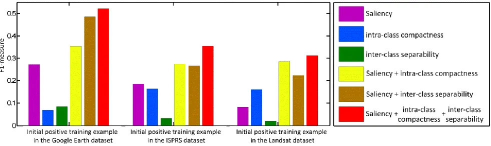
In this section, we evaluated the performance of the proposed Bayesian framework by comparing it with the baseline methods. Since the proposed Bayesian framework integrates the saliency, intra-class compactness, and inter-class separability information for the positive training example initialization (indicated by the bins in red in Fig. 9), we evaluated its performance on the training sets. Here, we treat the methods that initialize positive examples by using the saliency information only, the inter-class information only, the intra-class information only, fusing the saliency and inter-class information, and fusing the saliency and intra-class information as the baseline methods. Note that the last two baseline methods were also implemented by using the proposed Bayesian framework. Based on the criterion of F1-measure, the experimental results are shown in Fig. 9.
Fig. 9. Evaluation of the proposed Bayesian framework.
[image:19.595.51.542.570.716.2]20
results changes with the variation of the dataset and object of interest. For example, the saliency makes the biggest contribution for the initialization results on the Google Earth dataset whereas the intra-class information contributes mostly on the Landsat dataset; 2) in comparison to those using one of the three kinds of information, the performance of the fusion methods is more promising; and 3) fusion of all the three information always achieves the best results regardless to the variation of datasets and objects of interest.
6.4 Evaluation of the high-level feature
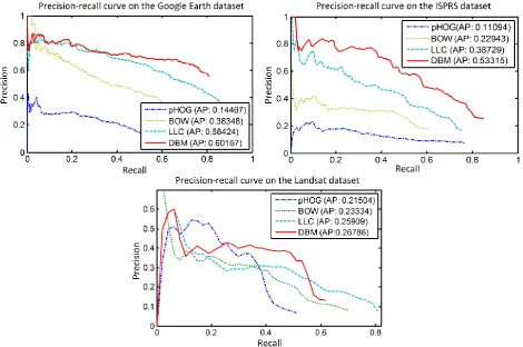
[image:20.595.62.533.370.682.2]In order to demonstrate the effectiveness of the proposed high-level feature, we compared it with three state-of-the-art features, which include the bag-of-word (BOW) [26], the pyramid histograms of oriented gradients (pHOG) [6][39] and the LLC [28]. Specifically, the BOW feature characterizes each training data by using a histogram of visual words; the pHOG feature represents the shape property of the image patches by using histograms of orientation gradients while the LLC feature is described in subsection 4.2. For quantitative evaluation, we plot the precision-recall (PR) curve of the object detection results and calculated average precision (AP) value as shown in Fig. 10 for comparisons. Specifically, the PR curve is plotted based on the values of PRE and REC under different thresholds while the AP is calculated by the area under the PR curve [3, 14]. The four different features were compared using the proposed WSL framework and the same sets of training and testing data. As shown in Fig. 10, the proposed high-level feature always outperforms the other three state-of-the-art features.
Fig. 10. Precision-recall curves for different types of feature on the three datasets. Here DBM indicates the high-level feature learned by the proposed work.
6.5 Evaluation of the object detector
21
with one existing WSL based method and several supervised learning based methods. Firstly, we compared the proposed approach with the WSL based method in [23]. For the fair comparison, in the experiment we utilized the same experimental settings including the same feature representation build by DBM, the same sliding window scheme, and the same testing image set. Fig. 11 gives the PR curves
[image:21.595.50.535.147.280.2]of the experiment results. The corresponding AP values are shown in Table Ⅱ.
Fig. 11. Precision-recall curves for the comparisons with the weakly supervised learning method.
We also compared the proposed WSL approach with several existing supervised learning based
object detection methods including a baseline method from Xu [26], and Han’s method [3]. The baseline
method was implemented by training object detector (linear SVM) based on the proposed high-level feature in a manner of fully supervised learning where the human annotations (manually labeled bounding box for each target in training images) are provided in the training images. The object detector trained by Xu’s method was based on the spectral and texture local feature descriptor and SVM with RBF kernel. Han's method trained object detector via discriminative sparse coding which has small within-class scatter and large between-class scatter. All comparison methods were evaluated using the same sets of training and testing data. Fig. 12 illustrates the PR curves of the experiment results. The corresponding AP values are shown in Table Ⅱ.
Fig. 12. Precision-recall curves for the comparisons with the supervised learning methods.
From Figs.11-12 and Table Ⅱ, we can observe that the proposed WSL approach can achieve
much better performance than the state-of-the-art WSL based method and comparable performance
with the state-of-the-art fully supervised learning based methods. Specifically, the object detection
[image:21.595.47.547.492.640.2]22
i.e., 0.088 (8.88%), 0.1499 (14.99%), and 0.024 (2.4%) in terms of AP in the Google Earth dataset, the
ISPRS dataset, and the Landsat dataset, respectively. More encouragingly, the proposed WSL approach
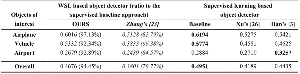
performs even better than other two state-of-the-art fully supervised methods in some cases. Specifically, for airplane detection in the Google earth dataset, it outperforms Xu’s method and Han’s method by 0.0741 (7.41%) and 0.0595 (5.95%), respectively. In the ISPRS dataset, the proposed WSL approach outperforms Xu’s method and Han’s method by 0.0751 (7.51%) and 0.0706 (7.06%), respectively. From the overall results among the three datasets, it can be seen that due to the powerful high-level feature representation built by DBM, the supervised baseline method yields the best results on these datasets. Benefited by the Bayesian framework to generate accurate initial training examples and the iterative training scheme to gradually refine the object detector, the proposed WSL algorithm achieves detection performance that outperforms the previous WSL based target detection method [23] and approaches to the fully supervised baseline method. Furthermore, based on the combination of the high-level feature representation and the proposed WSL framework, the overall performance of weakly supervised detector apparently outperforms the other two existing state-of-the-art supervised methods.
TABLE Ⅱ. DETAILED TARGET DETECTION RESULTS IN TERMS OF THE METRIC OF AP.
Objects of interest
WSL based object detector (ratio to the supervised baseline approach)
Supervised learning based object detector
OURS Zhang’s [23] Baseline Xu’s [26] Han’s [3]
Airplane Vehicle Airport
0.6016 (97.13%) 0.5332 (92.34%) 0.2679 (92.89%)
0.5128 (82.79%) 0.3833 (66.38%) 0.2439 (84.57%)
0.6194 0.5774 0.2884
0.5275 0.4581 0.2710
0.5421 0.4626 0.3257
Overall 0.4676 (94.45%) 0.3801 (76.77%) 0.4951 0.4189 0.4435
[image:22.595.39.557.300.428.2]Finally, some experimental results from the proposed approach for airplane detection, vehicle detection and airport detection are shown in Figs. 13-15, respectively. In these figures, the red rectangles indicate the true-positive results, while the black and yellow rectangles denote the false-positive and miss alarm results, respectively. As can be seen, the object detector trained via the proposed WSL approach can effectively detect objects of interest from all the datasets with different spatial resolution and cluttered backgrounds.
[image:22.595.48.517.550.752.2]23
Fig. 14. Examples of vehicle detection in the ISPRS dataset.
Fig. 15. Examples of airport detection in the Landsat dataset.
7.
Conclusions
In this paper, we have proposed a novel framework to tackle the problem of object detection in optical RSIs. The novelties that distinguish the proposed work from previous works lie in two major aspects. First, instead of using traditional supervised or semi-supervised learning methodology, this paper developed a WSL framework that can substantially reduce the human labor of annotating training data while achieving the outstanding performance. Second, we developed a deep network to learn high level features in an unsupervised manner, which offers a more powerful descriptor to capture the structural information of objects in RSIs. It thus can improve the object detection performance further. Experiments on three different types of RSI datasets have demonstrated the effectiveness and robustness of the proposed work.
[image:23.595.49.523.286.531.2]24
We will combine the rich spectral information provided by RSIs with spatial information for more accurate and robust object detection.
Acknowledgements: The authors would like to acknowledge the provision of the Vaihingen data set provided by the German Society for Photogrammetry, Remote Sensing and Geoinformation and the provision of Downtown Toronto data set by Optech Inc., First Base Solutions Inc., GeoICT Lab at York University, and ISPRS WG III/4. This work was partially supported by the National Science Foundation of China under Grant 91120005 and Doctoral Fund of Ministry of Education of China under grant 20136102110037.
8.
References
[1] W. Liu, F. Yamazaki, and T. T. Vu, “Automated vehicle extraction and speed determination from QuickBird satellite images,” IEEE J. sel. Topics Appl. Earth Observ. Remote Sens., vol. 4, no. 1, pp. 75-82, 2011.
[2] G. Cheng, L. Guo, T. Zhao, J. Han, H. Li, and J. Fang, “Automatic landslide detection from remote-sensing imagery using a scene classification method based on BoVW and pLSA,” Int. J.
Remote Sens., vol. 34, no. 1, pp. 45-59, 2013.
[3] J. Han, P. Zhou, D. Zhang, G. Cheng, L. Guo, Z. Liu, S. Bu, and J. Wu, “Efficient, simultaneous detection of multi-class geospatial targets based on visual saliency modeling and discriminative learning of sparse coding,” ISPRS J. Photogramm. Remote Sens., vol. 89, pp. 37-48, 2014. [4] X. Li, S. Zhang, X. Pan, P. Dale, and R. Cropp, “Straight road edge detection from
high-resolution remote sensing images based on the ridgelet transform with the revised parallel-beam Radon transform,” Int. J. Remote Sens., vol. 31, no. 19, pp. 5041-5059, 2010. [5] G. Liu, Y. Zhang, X. Zheng, X. Sun, K. Fu, and H. Wang, “A New Method on Inshore Ship
Detection in High-Resolution Satellite Images Using Shape and Context Information,” IEEE
Geosci. Remote Sens. Lett., vol. 11, no. 3, pp. 617-621, 2014.
[6] G. Cheng, J. Han, L. Guo, X. Qian, P. Zhou, X. Yao, and X. Hu, “Object detection in remote sensing imagery using a discriminatively trained mixture model,” ISPRS J. Photogramm.
Remote Sens., vol. 85, pp. 32-43, 2013.
[7] J. Han, S. He, X. Qian, D. Wang, L. Guo, and T. Liu, “An object-oriented visual saliency detection framework based on sparse coding representations,” IEEE Trans. Circuits Syst. Video
Technol., vol. 23, no. 12, pp.2009 -2021, 2013.
[8] J. Leitloff, S. Hinz, and U. Stilla, “Vehicle detection in very high resolution satellite images of city areas,” IEEE Trans. Geosci. Remote Sens., vol. 48, no. 7, pp. 2795-2806, 2010.
[9] X. Huang, and L. Zhang, “An SVM ensemble approach combining spectral, structural, and semantic features for the classification of high-resolution remotely sensed imagery,” IEEE Trans.
Geosci. Remote Sens., vol. 51, no. 1, pp. 257-272, 2013.
[10] P. Zhang, Z. Lv, and W. Shi, “Object-Based Spatial Feature for Classification of Very High Resolution Remote Sensing Images,” IEEE Geosci. Remote Sens. Lett., vol. 10, no. 6, pp.1572 -1576 2013.
[11] Y. Bengio, A. Courville, and P. Vincent, “Representation learning: A review and new perspectives,” IEEE Trans. Pattern Anal. Mach. Intell., vol. 35, pp. 1798–1828, 2013.
25
Int. Conf. Mach. Learn., 2012, pp. 1-8.
[13] R. Salakhutdinov, and G. E. Hinton, "Deep boltzmann machines," in Proc. Int. Conf. Artificial
Intelligence and Statistics, 2009. pp. 448-455.
[14] X. Bai, H. Zhang, and J. Zhou, “VHR Object Detection Based on Structural Feature Extraction and Query Expansion,” IEEE Trans. Geosci. Remote Sens., vol. PP, no. 99, pp. 1-13, 2014. [15] I. Dópido, J. Li, P. R. Marpu, A. Plaza, J. M. Bioucas Dias, and J. A. Benediktsson,
“Semisupervised self-learning for hyperspectral image classification,” IEEE Trans. Geosci.
Remote Sens., vol. 51, no. 7, pp. 4032-4044, 2013.
[16] W. Liao, A. Pizurica, P. Scheunders, W. Philips, and Y. Pi, “Semisupervised local discriminant analysis for feature extraction in hyperspectral images,” IEEE Trans. Geosci. Remote Sens., vol. 51, no. 1, pp. 184-198, 2013.
[17] E. Pasolli, F. Melgani, N. Alajlan, and N. Conci, “Optical image classification: A ground-truth design framework,” IEEE Trans. Geosci. Remote Sens., vol. 51, no. 6, pp. 3580-3597, 2013. [18] G. Jun, and J. Ghosh, “Semisupervised learning of hyperspectral data with unknown land-cover
classes,” IEEE Trans. Geosci. Remote Sens., vol. 51, no. 1, pp. 273-282, 2013.
[19] B. Alexe, T. Deselaers, and V. Ferrari, “Measuring the objectness of image windows,” IEEE
Trans. Pattern Anal. Mach. Intell., vol. 34, no. 11, pp. 2189-2202, 2012.
[20] T. Deselaers, B. Alexe, and V. Ferrari, “Weakly supervised localization and learning with generic knowledge,” Int. J. Comput. Vis., vol. 100, no. 3, pp. 275-293, 2012.
[21] P. Siva, C. Russell, and T. Xiang, "In defence of negative mining for annotating weakly labelled data," in Proc. Eur. Conf. Comput. Vision, 2012, pp. 594-608.
[22] P. Siva, and T. Xiang, "Weakly supervised object detector learning with model drift detection,"
in Proc. IEEE Int. Conf. Comput. Vision, 2011, pp. 343-350.
[23] D. Zhang, J. Han, G. Cheng, Z. Liu, S. Bu, and L. Guo, “Weakly Supervised Learning for Target Detection in Remote Sensing Images,” IEEE Geosci. Remote Sens. Lett., accepted.
[24] P. F. Felzenszwalb, R. B. Girshick, D. McAllester, and D. Ramanan, “Object detection with discriminatively trained part-based models,” IEEE Trans. Pattern Anal. Mach. Intell., vol. 32, no. 9, pp. 1627-1645, 2010.
[25] B. Sirmacek, and C. Unsalan, “Urban-area and building detection using SIFT keypoints and graph theory,” IEEE Trans. Geosci. Remote Sens., vol. 47, no. 4, pp. 1156-1167, 2009.
[26] S. Xu, T. Fang, D. Li, and S. Wang, “Object classification of aerial images with bag-of-visual words,” IEEE Geosci. Remote Sens. Lett., vol. 7, no. 2, pp. 366-370, 2010.
[27] D. G. Lowe, “Distinctive image features from scale-invariant keypoints,” Int. J. Comput. Vis.,
vol. 60, no. 2, pp. 91-110, 2004.
[28] J. Wang, J. Yang, K. Yu, F. Lv, T. Huang, and Y. Gong, "Locality-constrained linear coding for image classification," in Proc. IEEE Int. Conf. Comput. Vision Pattern Recognit., 2010. pp. 3360-3367.
[29] Y. Yang, and S. Newsam, “Geographic image retrieval using local invariant features,” IEEE
Trans. Geosci. Remote Sens., vol. 51, no. 2, pp. 818-832, 2013.
[30] L. Zhang, M. H. Tong, T. K. Marks, H. Shan, and G. W. Cottrell, “SUN: A Bayesian framework for saliency using natural statistics,” J. Vision, vol. 8, no. 7, pp. 32, 2008.
[31] I. Rigas, G. Economou, and S. Fotopoulos, “Low-Level Visual Saliency With Application on Aerial Imagery,” IEEE Geosci. Remote Sens. Lett., vol. 10, no. 6, pp.1389-1393, 2013.
[32] Z. Li, and L. Itti, “Saliency and gist features for target detection in satellite images,” IEEE Trans.
Image Process., vol. 20, no. 7, pp. 2017-2029, 2011.
26
Recognit. Lett., vol. 34, no. 11, pp. 1270-1278, 2013.
[34] C. M. Bishop, Pattern recognition and machine learning. springer, Aug. 2006.
[35] Y. Xie, H. Lu, and M. Yang, “Bayesian saliency via low and mid level cues,” IEEE Trans. Image
Process., vol. 22, no. 5, pp. 1689-1698, 2013.
[36] O. Boiman, E. Shechtman, and M. Irani, "In defense of nearest-neighbor based image classification," in Proc. IEEE Int. Conf. Comput. Vision Pattern Recognit., 2008. pp. 1-8.
[37] A. M. Cheriyadat, “Unsupervised Feature Learning for Aerial Scene Classification,” IEEE Trans.
Geosci. Remote Sens., vol. 52, no. 1, pp. 439-451, 2013.
[38] M. Cramer, “The DGPF-test on digital airborne camera evaluation overview and test design,”
Photogrammetrie-Fernerkundung-Geoinformation, vol. 2010, no. 2, pp. 73-82, 2010.
[39] F. Del Frate, F. Pacifici, G. Schiavon, and C. Solimini, “Use of neural networks for automatic classification from high-resolution images,” IEEE Trans. Geosci. Remote Sens., vol. 45, no. 4, pp. 800-809, 2007.
[40] A. Bosch, A. Zisserman, and X. Munoz, "Representing shape with a spatial pyramid kernel," in