Nonlinear parameter estimation in classification problems

Nonlinear Parameter Estimation

in Classification Problems

Kim Louise Blackmore

B.Sc. Hons University of Queensland

March

1995

A thesis submitted for the degree of Doctor of Philosophy at The Australian National University

Department of Engineering

These doctoral studies were conducted under the supervision of Dr Iven M.Y. Mareels and Dr Robert C. Williamson, with Prof. Darrell Williamson acting as advisor.

The contents of this thesis are the results of original research, performed in cooperation with Iven Mareels and Bob Williamson. Approximately 70% of the work is my own. The work on decision region approximation described in Chapter 6 was begun in response to discussions with Dr Peter Bartlett. Dr William A. Sethares participated in the work described in Chapter 7. The research described in this thesis has not been submitted for a higher degree at any other university or institution.

Sections of this work have been presented at conferences and submitted to journals, as detailed below.

Journal Papers:

(1)

Kim L. Blackmore, Robert C. Williamson, and Iven M.Y. Mareels, "Learning Nonlinearly Para:metrized Decision Regions", to appear in Journal of Mathemat-ical Systems, Estimation, and Control. Accepted November 1993.

(2) Kim L. Blackmore, Robert C. Williamson, and Iven M.Y. Mareels, "Local Minima and Attractors at Infinity in Gradient Descent Learning Algorithms", to appear in Journal of Mathematical Systems, Estimation, and Control. Accepted June 1994.

(3) Kim L. Blackmore, Robert C. Williamson, and Iven M.Y. Mareels, "Decision Region Approximation by Polynomials or Neural Networks", submitted to IEEE

Trans. on Information Theory in October 1994.

(4) Kim L. Blackmore, Robert C. Williamson, Iven M.Y. Mareels, and William A. Set hares, "Online Learning via Congregational Gradient Descent", to be submit-ted to Mathematics of Control, Signals and Systems in March 1995.

Conference Papers:

(5) Kim L. Halliwell, Robert C. Williamson, and Iven M.Y. Mareels, "Learning Non-linearly Parametrized Decision Regions", Proceedings of the Fourth Australian

Conference on Neural Networks, pp 74-77, 1993.

(6)

Kim L. Halliwell, Robert C. Williamson, and Iven M.Y. Mareels, "Learning Non-linearly Parametrized Decision Regions", presented at The 29th Australian Ap-plied Mathematics Conference (no proceedings), 1993.

(7)

Kim L. Halliwell, Robert C. Williamson, and Iven M.Y. Mareels, "Learning Non-linearly Parametrized Decision Regions", Proceedings of 12th World Congress of

the International Federation of Automatic Control, Volume 5, pp 431-434, 1993.

(8)

Kim L. Halliwell, Robert C. Williamson, and Iven M.Y. Mareels, "Local Minima

and Attractors at Infinity in Gradient Descent Learning Algorithms", Proceedings of the Fifth Australian Conference on Neural Networks, pp 161-164, 1994.

(9)

Kim L. Blackmore, Robert C. Williamson, and Iven M.Y. Mareels, "Decision Re-gion Approximation", Proceedings of the Sixth Australian Conference on Neural

Networks, pp 106- 109, 1995.

(10) Kim L. Blackmore, Robert C. Williamson, and Iven M.Y. Mareels, "Congrega-tional Gradient Descent", presented at ANZIAM'95-The Australian and New Zealand Industrial and Applied Maths Conference (no proceedings), 1995.

(11) Kim L. Blackmore, Robert C. Williamson, Iven M.Y. Mareels, and William A. Sethares, "Online Learning via Congregational Gradient Descent", to be pre-sented at COLT'95- The ACM Annual Workshop on Computational Learning

Theory, 1995.

Kim Louise Blackmore

A nonlinear generalisation of the perceptron learning algorithm is presented and

anal-ysed. The new algorithm is designed for learning nonlinearly parametrised decision

regions. It is shown that this algorithm can be viewed as a stepwise gradient descent of a certain cost function. Averaging theory is used to describe the behaviour of the algorithm, and in the process conditions guaranteeing convergence of the algorithm are

established. These conditions are hard to test, so some simpler sufficient are derived using the directional derivative of the instantaneous cost. A number of simulation examples and applications are given, showing the variety of situations in which the algorithm can be used.

In the initial analysis, a great deal of a priori knowledge about the decision region to be learnt has been assumed-in particular, it is assumed that the decision region is parametrised by some known (nonlinear) function. Often in applications, a general class of decision regions must be assumed, in which case the best approximate from the class is sought. It is shown that function approximation results can be used to derive degree of approximation results for decision regions. The approximating classes of decision regions considered are described by polynomial and neural network parametrisations.

One shortcoming of all gradient descent type algorithms, such as the online learning algorithm discussed in the first part of this thesis, is that estimates may be attracted to local minima of the cost function. This is a problem because local minima occur in many interesting cases. Therefore a modified version of the algorithm, which avoids local minima traps, is presented. In the new algorithm, a number of parameter estimates

( called a congregation) are kept at any one time, and periodically all but the best estimate are restarted. Convergence of the new algorithm is established using the

averaging theory that was used for the first algorithm. A probabilistic result concerning the expected time to convergence of the algorithm is given, and the effect of different population sizes is investigated. Again, a number of simulation examples are presented,

including the application to the CMA algorithm for blind equalisation.

Acknowledgements

So I have come to the end of my PhD studies. Many times I've doubted that this event would ever come, but here it is. It has been a time of great learning for me, and great growth as a person. Contrary to expectation, it has not been a terribly painful experience, give or take the odd deadline. In part, that is due to all the helpful people that have been around during my three years in Canberra.

First and foremost, my thanks go to my supervisors Bob Williamson and Iven Mareels. They have given me support, direction, advice and encouragement throughout my PhD studies. They have been a source of much information, and have always gone out of their way to give me time and attention when I've needed it. Thanks also to the students and staff of both the Department of Engineering and the Department of Systems Engineering, for friendship, entertainment, and sharing their insight into the world of engineering.

Throughout my studies I have received funding from the Australian Government through the Australian Postgraduate Research Awards, from ANUTECH, and from (CR)2 ASys. Without these funds I would not have been able to finish my PhD so quickly, and cer-tainly not so comfortably.

Of course much of who I am I owe to my parents. They have always encouraged me to think creatively about where I'm going and what I'm doing, and not to be bound by the establishment. I will always feel the warmth of their love. I am also grateful to Louise and Stephanie, who were my family for the first couple of years here in Canberra, and of course the members of the Westminster Presbyterian Church in Belconnen, who have provided love an support and ample distraction from my PhD studies. The most effective distraction, as well as the best motivation, has been provided by my husband and colleague Perry. Thankyou for never questioning my abilities. And for loving me.

Acts 17:28

Contents

1 Introduction

1.1

1.2

1.3

1.4

1.5

1.6

Neural Networks and Learning Algorithms .

Parameter Estimation in System Identification

Averaging Theory . . .

Approximation Theory .

Populational Algorithms

Contributions of This Thesis

1. 7 Things to Come . . . .

1.8 Relationship to Published Work .

2 Technical Matters

2.1 Notation and Definitions .

2.1.1 Stability in Dynamical Systems

2.2 Averaging Theory . . . .

Vl

1

2

6

7

8

10

11

13

15

17

17

22

3.2

3.3

3.4

3.5

. . . .

..

. . . .

.

Parametrisation . . . .

. . .

Algorithm Statement .

. . .

Cost Functions . . . .

. . . .

.

. . .

Algorithm Variations .

. . .

3.5.1

3.5.2

3.5.3

Gradient Descent on Jo . . .

Standard Parameter Estimation

Gradient Descent on the Misclassified Volume .

4 Algorithm Convergence - Unique True Parameter

4.1 Dynamical Systems Analysis

4.2

4.3

4.4

Testing for a Unique Critical Point

Examples . . . .

4.3.1

4.3.2

Learning a half space .

Learning a stripe .

Persistence of Excitation .

Correctly classified examples

. . .

4.4.1

4.4.2

4.4.3

Misclassified examples which cancel

Samples which do not span the parameter space

5 Algorithm Convergence - Multiple True Parameters

5.1

5.2

5.3

Dynamical Systems Analysis

Testing for Lagrange Stability

Examples . . . .

5.3.1

Learning a stripe

64

65

66

70

70

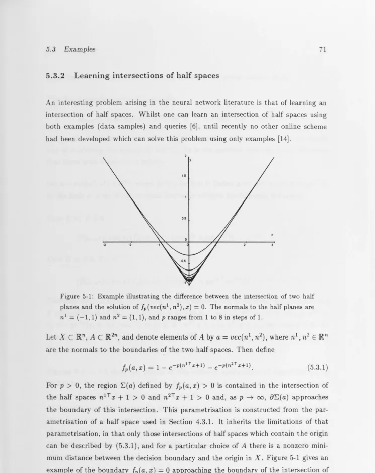
5.3.2 Learning intersections of half spaces . . . 71

6 Decision Region Approximation

6.1

6.2

6.3

6.4

The Approximation Problem .

Construction of a Smooth Discriminant

Polynomial Decision Regions

Neural Network Decision Regions

7 Congregational Gradient Descent Algorithm

7.1

7.2

7.3

Algorithm Statement . . . .

Analysis for a Simpler Case

Dynamical Systems Analysis

76

77

80

82

84

87

88

91

93

7.4 Expected Time to Convergence . . . 104

7.5 An Example . . . .. . . 107

8 Conclusions ₁₁₀

.1 Further Work- Learning Decision Regions . . . 112

8.2

8.3

Further Work- Decision Region Approximation .

Further Work- Congregational Gradient Descent

A Technical Appendix

B Code for the Simulations

. . .

113

. . .

114

123

Chapter

1

Introduction

While many tasks can be achieved by programming a computer to follow a sequence of commands, ·computer scientists have long been interested in more closely _matching computer abilities to human intelligence. A primary abili~y of human intelligence is the ability to generalise inferences or actions from a restricted set of data to a broader one. Thus we can read another's handwriting if we have seen it often enough, and we can instantly recognise faces, even though expressions and features change. Moreover, specialists operate according to acquired intuition specific to their field. Consider for instance a psychologist identifying potential problems amongst a company's employees, a tycoon playing the stock-market, or an operator controlling some aspect of a chemical processing plant.

The problem of designing computers which are able to generalise from examples for the purpose of correct classification of data fits into the broad category of Artifical Intelligence. In particular, it is the subject of much research in the field of artificial neural networks. The approach to classification problems that is taken in this thesis is motivated by, but not restricted to, certain aspects of the artificial neural network literature. Artificial neural networks and learning algorithms are discussed further in Section 1.1.

The classification learning problem is closely related to the problem of parameter es-timation for system identification in automatic control and signal processing. In the formulation used in this thesis, the main difference between the two problems arises from the binary nature of classified data, as distinct from the real valued output from many systems. See Section 1.2 for a discussion of parameter estimation in system

identification. Techniques from the parameter estimation literature are used in investi-gating the behaviour of the learning algorithms proposed in this thesis. In particular, the powerful technical tool of averaging theory ( discussed further in Section 1.3) forms the basis of much of the algorithm analysis that is presented.

All parameter estimation problems assume some a priori knowledge about the structure of the rule to be learnt ( or the system to be identified). In practical situations such a priori knowledge is usually not available. However it can be shown that, under more reasonable general assumptions, there exist certain classes of structures which are good approximators. If the parameter estimation is for the purposes of matching a continuous function, this reduces to the problem of function approximation. For classification problems, the related problem of decision region approximation must be addressed. See Section 1.4.

Neural network learning, system identification and signal processing all use techniques from the broad mathematical field of optimisation. The algorithms discussed in this thesis are based on the classical gradien.t descent technique of optimisation. One class of more modern optimisation techniques, genetic algorithms, is discussed in Section 1.5. The desire to compare gradient descent type schemes with genetic algorithms was a major motivation for the latter part of the work presented in this thesis.

The contributions of this thesis are summarised in Section 1.6 and the structure of the thesis is outlined in Section 1.7. Section 1.8 details the relationship between this thesis and the papers arising from the research reported herein.

1.1

Neural Networks and Learning Algorithms

Certain pattern recognition problems can be set in the context of classification-events or other pieces of information are represented as points in n-dimensional space, referred to as sample space or feature space, and they are classified in some manner. The computer is given a sequence of examples of correctly classified points and is expected to learn to correctly classify all points in the space [72].

The classification problem described above is called supervised learning because a "teacher" is giving the "pupil" information as to the correct classification of received

1.1 Neural Networks and Learning Algorithms 3

learning schemes are also studied, such as the Self-Organising Map for neural networks [42]. In this thesis only supervised learning problems are considered.

Moreover, here it is assumed that there are just two possible classifications of an exam-ple, and the examples are described as being either positively or negatively classified. The set of all positively classified examples is called the decision region. This is not a inhibitive restriction because a larger number of classes can be learnt by subdividing the problem- each class can be learnt separately, with points classified according to inclusion or otherwise in the class currently under consideration. However if there are

more than two possible classifications, it may be beneficial to use a more complicated

algorithm.

Much research in the field of artificial intelligence has been motivated by the attempt

to model the behaviour of the human brain. This line of attack lead to the development

of artificial neur~l networks (ANNs). An artificial neural network is a highly connected

array of elementary processors referred to as neurons. In feedforward ANNs, the neu-rons are arranged in layers and each neuron only receives inputs from the layer above

it. The output of each neuron is given by

y(x(l), ... , x(n))

=

a

(t

a(i)x(i)

+Ii) ,

(1.1.1)

where then inputs

x(i)

are combined using

n+l

weights

a(i), 0,

and a is a memoryless

nonlinear function which satisfies

lim

a(x)

==

1

x-+oo x-+-oo lim

a(x)

==

-1.

Sometimes the lower limit for

a(·)

is assumed to be O rather than -1. If the function

a : IR-+ IR is continuous and monotonic it is called a sigmoid activation function. Often

the hyperbolic tangent function

a( x)

==

tanh

x

is used. If the artificial neural network

is to classify points the network must have binary output. This is achieved by using

the signum activation function

a(x)

==

{l

-1

if X

>

0

otherwise.

(1.1.2)

One of the first neural networks to be studied in depth was the perceptron, which is a

single layer neural network [60], and is closely related to the Adaline, or ADaptive Lln-ear NEuron [80]. In 1962, Rosenblatt [64] proposed the perceptron lLln-earning algorithm,

The perceptron is given a sequence of training examples {xk, Yk}kENo, where Xk E ]Rn

and Yk

=

±1 is the correct classification of x k. At any instant, parameters a( i) and (}

in (1.1.1) form the augmented vector ak

=

(a(l), ... , a(n), 0) and the sample Xk can be used to create the augmented vector Xk

=

(x(l),

...

,

x(n), 1). The signum activation

function (1.1.2) is used, so the output of the perceptron is y(xk)

=

sgn(al Xk). The parameters are updated according to the rule

(1.1.3)

otherwise,

where µ E (0, 1] is some stepsize. If the perceptron correctly classifies the point x k then no update is made, so the parameters stop updating if all of the training examples are

correctly classified.

It has been shown [60] that if the samples cycle periodically through a finite set of

points the perceptron learning algorithm will correctly classify all of those points after

a finite number of iterations of (1.1.3), provided the positively and negatively classified

points are linearly separable ( defined below). Other analyses of the perceptron learning

algorithm appear in [70, 68, 69].

Two sets A, B C ]Rn are said to be linearly separable if there exists a vector b E ]Rn

and a scalar (3

>

0 such that

T

{>

(3 b X

<

(3

for all x E A

for all x EB.

In many interesting cases, classes are not linearly separable, so a simple perceptron will

never be able to correctly classify all points. One way to deal with this problem is by

preprocessing the inputs [57, 62, 72]. For instance, if the decision region is a circle in 1R2,

centred at the origin, then positively classified points satisfy

(x(l)-k)

2_+(x(2)-l)2

_<

_r

for some k, l

E

JR and r

>

0. Replacing x

E

JR2 _with

_(x(l),

_x(1)2

,

x(2),

x(2)2)

E

JR4 and

letting b = (-2k, 1, -21, 1) and (3 = r - k2

- l2 gives a linearly separable problem. Such

pre-processing methods can only be applied if points are classified according to some relation that is linear in the parameters.

For general nonlinear decision regions, multilayer neural networks are often used. A two

layer feedforward neural network with a single hidden layer satisfies the input-output

relation

1.1 Neural Networks and Learning Algorithms 5

where m E N, x, aj E Rn and aj, /3j, ₁ E R for all j E (1, ... , m). Neural networks with further hidden layers can be defined iteratively. The back-propagation algorithm

that was popularised by Rumelhart et al. [65] is used for training multilayer neural networks. If the hyperbolic tangent sigmoid function is used, back-propagation for a

single neuron yields

(1.1.5)

Back-propagation is stepwise gradient descent on an error function. That is, the error

function is the average over the samples Xk of an instantaneous error function. As each

sample is received, the parameters are updated in the direction of steepest descent of

the instantaneous error function. If the update parameter is sufficiently small, this provides a good approximation to gradient descent on the average error function. Note

that the update parameter µ is held fixed in stepwise gradient descent, as distinct

from stochastic gradient descent ( or "stochastic approximation"), where the update

parameter is allowed to decay to zero.

The word "back-propagation" refers to the process by which the gradient of the

instan-taneous error function is propagated back through the network to determine the amount

that the weigh~s on each neuron should be updated. In [75], Sontag and Sussmann use

ordinary differential equations to give' a deterministic analysis of the back-propagation

algorithm. It has been found that the back-propagation algorithm exhibits both

conver-gence to non-global local minima and diverconver-gence to infinity in many applications [43].

Sontag and Sussmann have shown that the error function can exhibit local minima

for particular periodic input sequences [74]. Guo and Gelfand [32] provide a

quasi-linear analysis for multi-layer neural networks that gives insight to the behaviour of the

back-propagation algorithm.

Whilst they are widely used and discussed, neural networks are certainly not the only

method for describing nonlinear decision regions. There is some theoretical evidence to

show that neural networks are good function approximators, so they can be confidently applied to many general problems (see Section 1.4), but this is also true of rather

simpler classes of functions such as polynomials and rational functions. Moreover, in

some cases there may be a priori knowledge about the shape of the decision region, but

there is no way to incorporate this information into the neural network framework.

In this thesis a general decision region parametrisation (input-output relation) has been assumed, namely

y(x)

=

sgn(f(a,

x)),

where

f :

Rm-+ IR is a nonlinear function

a E JR m such that all points are correctly classified by

f

(

a, ·). The parameter vector

is analogous to the set of weights in the neural network context. A stepwise gradient descent algorithm for learning in this framework is presented and analysed.

1.2 Parameter Estimation in System Identification

Parameter estimation for system identification purposes is an important aspect of adap-tive control [1, 10], and equalisation in adaptive signal processing [40]. Parameter es-timation differs from classification in that the input-output relationship of the system is determined by a continuous, real valued function, rather than a binary valued clas-sification. Thus the input x is related to the output y according to some function

y(·)

=

J(a*,·),

where

a*

E lRm is the parameter to be identified. Note that the vector input x may be defined by a delayed sequence of scalar signals. Typically there is some error in the measurements of the input and output, so the parameters must be esti-mated on the basis of the noisy measurements

xk+~k

and

y(xk)+(k

[77, 49]. In many cases, the function

f

is assumed to be linear, but some research has centred around parameter estimation for nonlinear system models [7, 63].

Many parameter estimation techniques are based on the idea of output error min-imisation. The current estimate parameter is used to generate the estimate output

Yk

=

f(ak, Xk

+

~k),

and the output error to be minimised is

l K-1

J(a)

=

lim

K

I:

(y(xk)

+

(k -

Yk)

2. K-+oo .

i=O

(1.2.1)

The simplest such algorithm, used for linear systems, is the least mean squares algo-rithm (LMS), which reduces to

(1.2.2)

in the noise-free case. Convergence of the LMS algorithm is guaranteed because it is stepwise gradient descent of a quadratic (and hence convex) cost function [40].

1.3 Averaging Theory 7

linear systems have been proposed and analysed [1, 53, 30]. Many of the variations on stepwise gradient descent used in these algorithms could be profitably applied to the nonlinear classification problem considered in this thesis. The purpose of this thesis is not to examine particular variants of gradient descent based learning algorithms, but rather to present an in depth study of one such algorithm, with the aim of dis-playing issues which arise for nonlinear parametrisations that do not occur for linear parametrisations.

Lyapunov stability theory has long been used in the analysis of parameter estimation techniques [61, 47]. More recently this has been combined with averaging theory (see Section 1.3) for deterministic analysis of parameter estimation techniques, and with stochastic methods due to Kushner [50] to give stochastic analysis of parameter

esti-mation techniques [52, 13].

The connections between neural network learning and parameter estimation have not es-caped notice. Some authors have used neural network parametrisations for system mod-els, and then used neural network-specific learning algorithms such as back-propagation for parameter estimation [16, 54, 15, 71]. On the other hand, Kuan and Hornik [48], Finnoff [26], Heskes and Kappen [34], and Leen and Moody [51] have used the tech-niques due to Kushner to perform stochastic analyses of learning algorithms. In [14]

Bucklew and Sethares give a stochastic analysis of adaptive algorithms for learning

decision regions, where the problem formulation and proposed algorithm is very similar to the problem and algorithm in this thesis. Stochastic analyses of learning algorithms give results which are similar in flavour to the PAC model of learning that arises in

com-putational learning theory [78, 2], although the results are usually not strong enough to qualify strictly for that description.

1.3 Averaging Theory

Averaging theory is a tool for investigating the behaviour of a dynamical system by relating it to a less complicated system. This is achieved by considering the dynamics of the original system over two time scales-the long time scale describing the average behaviour of the system, and the shorter time scale describing the perturbations due

to some time-varying input. In the context of astronomy, the averaged system may describe the motion of a planet orbiting a sun, and the perturbation may be due to another planet in the solar system. In the context of output error minimisation for parameter estimation, the averaged system describes the minimisation of the average output error defined in (1.2.1), and the perturbation is due to the particular input

sequence (xk).

To describe the average behaviour of the system, the short time scale perturbations are omitted, giving an averaged system. The averaged system is time independent, and analysis of the system is simpler than the time-dependent case. The solution of the original system is shown to be a perturbation of the solution of the averaged system.

Thus, in the context of a parameter estimation algorithm, an update parameter (called the "stepsize") is chosen small enough that the parameter estimates ak vary slowly

com-pared to the inputs Xk. The averaged system is determined by averaging the parameter

update over all possible inputs, for each possible parameter estimate. In particular, averaging theory provides justification for stepwise gradient descent techniques, where parameters are updated by moving down the gradient of an instantaneous cost function, in order to locate the minima of an averaged cost function.

1.4

Approximation Theory

In the framework of this thesis, decision boundaries are represented as zero sets of certain functions, with points contained in the decision region yielding positive values of the function, and points outside the decision region yielding negative values. In

this case, the learning task is to use examples of correctly classified points to identify parameters a E lRm for which the set {x : f(a, x)

>

O}, called the positive domain of

f (a,·)

matches the true decision region, where

f

is some known function.

1.4 Approximation Theory 9

there is no general reason why such an assumption is satisfied in practice. Even if

a suitable function

f

exists for a particular decision region, there is usually no way of identifying this function a priori. It is therefore useful to know how well particular

classes of functions can approximate decision regions with prescribed general properties.

In particular, it is important to know how fast the approximation error decreases as

the approximating class becomes more complicated-e.g. as the degree of a polynomial

or the number of nodes of a neural network increases.

The question of approximation of functions has been widely studied. The classical

Weierstrass Theorem showed that polynomials are universal approximators [55] (in the

sense that they are dense in the space of continuous functions on an interval). Many

other classes have been shown to be universal approximators, including those defined

by neural networks [37, 38]. Other theoretical questions involve determining whether

or not best approximations exist and are unique [17, 81]. There are also degree of

approximation results, which tell the user how complicated a class of approximating

functions must be in order to guarantee a certain degree of accuracy of the best

ap-proximation. The classical Jackson Theorem [17] is the first example of this. Hornik

[38], Barron [4], Mhaskar and Michelli [59], Mhaskar [58], and Darken et al. [19] give

degree of approximation results for neural networks. Even more powerful results give

the best class of functions to use in approximating particular classes of functions, by

showing converses to Jackson type theorems for certain classes of functions [76].

The problem of approximating sets, rather than functions, has received some attention

in the literature. Work can be grouped according to two basic approaches-namely

explicit and implicit parametrisations. "Explicit parametrisation" refers to frameworks

where the decision boundary is parametrised. For example if the decision region is a

set in Rn, the decision boundary might be considered the graph of a function on Rn-1,

or a combination of such graphs. "Implicit parametrisation" refers to frameworks ( as

used in this thesis) where the decision region is the positive domain of some function.

Most existing work is in terms of explicit parametrisations [44]. For instance, Korostelev

and Tsybakov [45, 46] consider the estimation (from sample data) of decision regions.

Although they consider non-parametric estimation, it is in fact the explicit rather than

implicit framework as defined above (they reduce the problem to estimating functions

whose graphs make up parts of the decision boundary). In a similar vein, Dudley [24]

and Shchebrina [67] have determined the metric entropy of certain smooth curves.

vision purposes [8, 82].

Regarding the implicit problem, Mhaskar [58] gives a universal approximation type result for approximation by neural network decision regions. It appears that the ar-gument in [58] can not be used to determine the degree of approximation. Ivanov [39] summarises many problems in algebraic geometry concerned with the question of when a smooth manifold can be approximated by a real algebraic set but does not address the degree of approximation question. In work similar to that described in [39], Broglia and Tognoli [12] consider when a C00 _{function can be approximated by certain classes}

of functions without changing the positive domain.

In this thesis function approximation results are used to determine the degree of ap-proximation of decision regions by positive domains of polynomial functions and certain neural network functions. Approximation error is measured in terms of the volume of the misclassification region, which can be interpreted as the probability of misclassifi-cation by the approximate decision region, when the data are drawn from a uniform distribution over the input space.

1.5

Populational Algorithms

The problem of optimisation is concerned with identifying minima ( or maxima) of some cost function. Stepwise gradient descent (SGD) is a classical discrete time optimisa-tion technique. Gradient descent methods find local minima of the cost function, and are only guaranteed to find the global minimum if estimates originate in the basin of attraction of the global minimum.

Genetic algorithms (GAs) are a more modern class of optimisation techniques, based on a hypothesised model of biological evolution. The basic idea of GAs involves the evolution of a population of estimates using principles of variation, selection, and in-heritance. The estimates are represented as binary strings of set length. Estimates are randomly initialised, varied, then tested for fitness (the value of the cost function is evaluated). The weakest members in the population are removed and new members are initialised to keep a constant population size. Again estimates are varied and tested, and the process continues [27]. Different rules for varying the estimates (including crossover and random mutation) and for initialising new members (such as making

•

•

••••---

---

---~cc

1.6 Contributions of This Thesis 11

A key difference between gradient descent methods and genetic algorithms is that mul-tiple estimates are simultaneously updated in GAs, whereas only a single estimate is used in classical gradient descent techniques. Another key difference is that in GAs the estimates are represented as binary strings and rules governing the variation of the estimates depend on the binary structure of the estimates.

In this thesis a populational version of stepwise gradient descent is proposed and anal-ysed. The new algorithm is motivated by the observation that in problems such as the decision region learning problem addressed in the first part of this thesis, a differentiable instantaneous cost function naturally arises. If a GA were used for optimising such a cost function, a mapping for the binary coding of the estimates must be chosen. In the process, the differentiable structure of the problem is lost. On the other hand, if only a single estimate is used for gradient descent, there is no guarantee that the estimate will not get stuck in a local minimum or wander off to infinity. Large deviations theory suggests that. the estimate will eventually escape from local minima, and is less likely to escape from the global minimum. However the estimate cannot be expected to escape an attractor at infinity [28, 34].

The populational SGD algorithm presented in this thesis combines the GA idea of survival of the fittest with the classical gradient descent technique for variation of estimates between testing for fitness. It is perhaps the simplest conceivable populational SGD algorithm. It seems that simple populational SGD algorithms do not appear elsewhere in the literature. One exception is the "multistart" algorithm described in [85] (pp. 24ff). This algorithm works when one has a fully known cost function, rather than just samples of it, and is somewhat different to the algorithm in this thesis in other ways. Certainly the analysis in this thesis is different to that presented by Zhigljavsky. Another is "Branin 's method" [85] (pp. 32-33), which is essentially a deterministic method of escaping from local minima in descent algorithms.

1.6

Contributions of This Thesis

estimation problems.

The convergence properties of both algorithms are investigated and the viability of certain nonlinear parametrisations of decision regions is established via decision region rate of approximation results. For the second algorithm, a probabilistic estimate of the time to convergence is established. A number of applications from learning, regression and signal processing are discussed.

The work pertaining to the SGD learning algorithm is new in several ways:

• The class of decision regions that can be learnt is very general, being described by positive domains of differentiable nonlinear functions.

• The analysis of the algorithm uses deterministic averaging theory, so the conver-gence result is deterministic.

• As in certain neural network structures (e.g. equation 1.1.4), a sigmoidal squash-ing function is used in comparsquash-ing the output of the parametrisation with the correct classification.' In the process of the analysis, it is made clear that the

steepness of the sigmoidal squashing function must be linked to the stepsize µ of the learning algorithm in order to guarantee that the algorithm converges exactly in the limit µ -+ 0.

• Techniques for investigating the topological properties of the average cost func-tion, and hence the behaviour of the parameters derived from the learning algo-rithm, are provided. Application of these techniques is demonstrated for specific parametrisations.

The decision region rate of approximation results are, to our knowledge, the first such results to appear. Indeed, it seems that very little discussion of the difference between

function approximation and decision region approximation has appeared in the liter-ature. A simple convolution technique is provided which makes it possible to apply degree of approximation results from £00 function approximation.

The congregational gradient descent algorithm is also new. To our knowledge, it is the

1. 7 Things to Come 13

its gradient can be calculated at each time instant. The analysis of the congregational

algorithm is new in that:

• Deterministic averaging theory is combined with probability theory, since the inputs Xk are assumed fixed but the initial parameter estimates are assumed to

be random variables.

• The expected time until convergence of the algorithm is determined as a function of the number of members in the parametrisation and the size of the basin of

attraction of the global minimum.

• It is shown that there is an optimal number of members in the congregation. Unless the basin of attraction of the global minimum is very small, the optimal

number of members is very small. However the saving in computation achieved

by using the optimal number of members, rather than just two members, is also

small ( a factor of

! ) .

This contrasts with the genetic algorithm situation, where very large populations are used [3, 29].

The congregational algorithm is successfully applied to the problem of blind equalisation

of a linear communications channel using the Constant Modulus Algorithm (CMA).

This is significant because it is known that CMA suffers from ill-convergence due to

local minima in the cost function [21], and techniques for identifying ill-convergence

and restarting the algorithm is an active topic of research [23, 22].

1. 7

Things to Come

Chapter 2 is a fairly dry technical chapter, which could initially be read only briefly. In

Section 2.1 the notation used in this thesis is presented and much of the terminology is

defined. Most of the notations and definitions are standard in the literature, but some

terminologies are slightly nonstandard. These variations, together with the reason for making them, are discussed with the definitions.

In Section 2.2, the results from averaging theory that are needed for the analysis in

this thesis are presented. The results that are needed are an extension of the existing

used in the algorithm analysis in later chapters, so that results and assumptions are frequently referred to in the text.

In Chapter 3, the classification problem is stated and a formal definition of a online

learning algorithm for solving classification problems is given. The concept of a

par-ametrisation for a class of decision regions is also formally defined. On this basis, the

SGD algorithm for learning is presented, and it is shown that this algorithm is closely

related to the perceptron learning algorithm. The average cost function governing the

behaviour of the algorithm is discussed and a number of possible variations of the

algorithm and the cost function are outlined.

In Chapter 4, the first stage of the analysis of the SGD learning algorithm is presented.

Conditions are given which guarantee that the algorithm is indeed an (approximate)

online learning algorithm. One key condition is that the average cost function has a

unique critical point. The assumptions which are used in this analysis are discussed,

and alternative sufficient conditions, which are easier to test, are derived using the

concept of the directional derivative of a function. The application of the algorithm to

learning a half space and a stripe is presented, and the importance of an information

rich training sequence is discussed.

In Chapter 5, further analysis of the SGD learning algorithm is presented, with the

assumption of a unique critical point of the cost function relaxed to allow for multiple

isolated critical points. Again, the directional derivative is used to simplify the new

conditions, this time deriving methods for testing for Lagrange stability of the averaged

ordinary differential equation. The application of the algorithm to learning a stripe is

discussed further, and the application to learning an intersection of two half spaces is

demonstrated.

In Chapter 6, decision region rate of approximation results are presented. Concepts

from differential geometry are used to connect the volume of the misclassified region

with the distance between the true and estimate decision boundaries. A

convolu-tion process is used to construct a continuous function whose positive domain closely

matches the decision boundary. Rate of function approximation results are applied to

this continuous function, giving a bound on the volume of the misclassified region.

Ap-proximating decision regions which are described by either polynomials or two hidden

layer neural networks are considered.

1.8 Relationship to Published Work 15

that this algorithm can be applied to, but is not restricted to, the decision region learning problem. Using averaging theory and basic probability theory, a probabilistic convergence result is derived. A formula for the expected time to convergence is derived, and this formula is used to analyse the expected amount of computation required by the algorithm. From this analysis, it is shown that for each cost function there is an optimal number of members. It is also shown that using two members in the congregation, rather than the optimal number, will result in an algorithm which will not use more than twice as much computation. The congregational algorithm is applied to the problem of blind equalisation of a linear communications channel using the Constant Modulus Algorithm.

Conclusions and areas for further research are discussed in Chapter 8.

1.8

Relationship to Published Work

Sections of the work described in this thesis have been presented at various conferences and submitted to journals. A list of the relevant papers appears immediately after the title page. There are some differences between the published papers and this thesis, particularly in the analysis of Algorithm 3.1. In this section, the relationship between the work described in this thesis and in the listed papers is described for the benefit of readers who have already read some of the papers.

The averaging theory results that appear in Section 2.2 are similar to the results that appear in the appendix of paper ( 4)-"0nline Learning via Congregational Gradient Descent". However the main result here is more general because it allows convergence to an invariant set, rather than a critical point. Moreover, here the update in the unaveraged equation is allowed to depend on the stepsize µ is a more complicated manner than in that paper.

Chapters 3 through 5 are closely related to paper (1)-"Learning Nonlinearly Paramet-rised Decision Regions" and its sequel, (2)-"Local Minima and Attractors at Infinity in Gradient Descent Learning Algorithms". Algorithm 3.1 is the online learning algo-rithm that appears in both of these papers, and the results and analysis techniques are of a similar nature.

presented. However, the averaging theory used in (1) is weaker than what is used here--the difference equation defined by Algorithm 3.1 is linked with a time dependent ODE and continuous time averaging theory is used. In this thesis the difference equation defined by Algorithm 3.1 is linked directly with the averaged ODE in the averaging theory. This direct linkage is both conceptually simpler and more elegant.

The direct linkage between the Algorithm 3.1 and the averaged ODE has enabled the analysis in Sections 4.1 and 5.1 to be tightened further by linking the boundary sensitivity c the stepsize µ in an explicit manner. This ensures convergence to the true parameter value, rather than an

oe(l)

neighbourhood of the true parameter value. Moreover, in (1) the cost Je is considered, but the limiting cost J0 is not discussed. The discussion of the cost surface Jo in Section 3.4 contributes significantly to the intuitive understanding of the behaviour of the algorithm.

Sections 4.2 and 5.2 are closely related to parts of (2). However, in (2) the cost function Je is considered, whereas here the cost function J0 is used. Again, the use of / 0 rather than Je contributes t_o the intuitive understanding of the re~ults presented.

The conference papers (5), (6), and (7) are early versions of the work presented in (1). They included an erroneous statement of the cost function governing Algorithm 3.1. In particular, it was claimed that the cost function is

Ge,

as defined in equation 3.5.5. Consequently, in the followup paper (8), the cost function

Ge

was used instead of

Je.

In all cases, the nature of the results is not changed, but the stathent of the results appears significantly different.

Chapter

2

Technical Matters

Before moving on to the main body of the thesis, notations and definitions that are used throughout the thesis are detailed in Section 2.1, and a key result from averaging theory (Theorem 2.1) is derived in Section 2.2. Theorem 2.1 is a new, but relatively straightforward, generalisation of existing results. This result is central to the analysis of Algorithms 3.1 and 7.1 that appears in Chapters 4, 5 and 7. Most of Section 2.2 is taken up with technical proofs, which can be omitted without detracting from the logical flow of the thesis.

2.1

Notation and Definitions

Real and natural numbers: The real numbers are denoted JR, and the set of non-negative real numbers is JR+ := { x E JR: x

>

O}. The natural numbers are denoted N,

and No := {O, 1, 2, ... } is the set of natural numbers plus zero.

Norms: For any vector

x

E JRn, if i E {1, ... , n} then

x(i)

denotes the i-th component of x, and llxll denotes the Euclidean norm (2 norm). For any real n x n matrix y, the

(induced) norm of y is

IIYII

=

supllxll=l llyxll·

Matrix inequalities: Let x and y be n x n symmetric real matrices. x is less than or equal toy (x

<

y) if y - x is positive semi-definite.

Equivalent functions: Functions

f,g:

]Rn -+ ]Rm are equivalent if

f

(x)

=

g

(x)

for

all x E lRn. This is written/(·)= g(·).

Gradient and Hessian of a function: For any function

f (

a, x) :

A x X -+ JR, where Ac ]Rm and X C ]Rn,

M

denotes the gradient off with respect to the first argument,

and ~:{ denotes the Hessian matrix, of

f

with respect to the first argument.

For any p E N, a p-th order derivative off : lRn-+ JR is D 0

f

= ax(i)a(1)ax(2

f

!(2)

...

ax(n)a(n),

where a is any vector a E

Na

such that

Li=l

a(

i)

= p.

Integration: The Lebesgue integral is used for all integration in this thesis.

Quasi-convex: A function

f :

]Rn -+ JR is quasi-convex if, for all x1, x2 E ]Rn and

A

E [O, l],

f(Ax1

+

(1 -

A)x2)

<

max{f(x1), f(x2)}.

Open ball and cube: The open ball with centre x E ]Rn and radius r

> 0 is denoted

B(x, r).

The open n-cube with centre

x

E ]Rn and side

s

>

0 is

I(x, s)

:=

{y

E ]Rn :

I

y ( i) - x ( i)

I

< ~, i

=

1, ... ,

n}.

0

Set notations: For any set D C ]Rn, D denotes the interior of D, 8D denotes the

boundary of D, and D denotes the closure of D. The diameter of D is given by

diam D := SUPx,yED

llx -

YII-

The volume of a compact set DC ]Rn is vol D :=

JD

dx.

For D1,D2 E lRn, the set of points in D1 but not in D2 is D1\D2 :=

{x

E D1:

x

r/.

D2},

and the symmetric difference of D 1 and D2 is D16.D2 := D1 \D2

U

D2 \D1. A sequence of sets Di C lRn, i in some index set J, are pairwise disjoint if Din Dj =

0

for all i,j E J.

Distance between a set and a point: The distance between D C ]Rn and x E ]Rn

is

d(D

x) := infyED llx -

YII·

The distance between a set and a point is used in Section

2.1.1 for describing stability properties of an invariant set in dynamical systems.

Hausdorff distance between sets: The Hausdorff distance between sets D1 C ]Rn

2.1 Notation and Definitions ₁₉

Delta corridor around a set: For any 8

>

0, the 8 corridor around D C ]Rn is the

set

D

+

8 :={y E JRn:

d(D,

y)

<

8} =

LJ

B(x,

8). xED

The 8 corridor around the decision boundary is used in Chapter 6 in relating function approximation to decision region approximation.

Corridor size between sets: _{The corridor size from D 1} C ]Rn to D 2 C ]Rn is p(D1, D2) := sup

d(8D1, x)

= inf{8: 8D2 C 8D1

+

8}.

xEBD2

The corridor size is not symmetric, so it is not a metric. The Hausdorff distance between the boundaries of D1 and D2 is max{p(D1, D2), p(D2, D1)} (which is a metric). The corridor size is used in Chapter 6 for measuring the distance of an approximate decision boundary from the true decision boundary.

Convergence of sets: Let

D, Dµ

C Rn be open for allµ

> 0. The sets

Dµ

converge to

D

as µ -+ 0 if limµ-+-0

H(D, Dµ)

-+ 0. This is written

Dµ

-+

D

as µ -+ 0, or

lim

Dµ

=

D.

µ-+-0

Covering sequence: A sequence (xk)kEZ+ of elements of a compact set X C Rn is a covering of X if, for any measurable function

f :

X -+ IR,

1 K-1 1

1

lim -

I:

f(xk)

=

1 f(x)dx.

K-+-oo

K

k=O VO

X

X

(2.1.1)

A covering in a deterministic framework is equivalent to a uniform distribution in a stochastic framework. In analysing the SGD learning algorithm presented in Chapter 3 and the congregational algorithm presented in Chapter 7, it is assumed that the sequence of samples input to the learning algorithm covers the sample space. Thus the cost function averaged over the input sequence is equivalent to the same function integrated over the sample space.

Comparison of order functions: Let

h(µ)

and

l(µ)

be order functions. Then the notations

Oµ(l(µ)), oµ(l(µ))

and

0.µ(l(µ))

are defined by

l.

h(µ)

=

Oµ(l(µ))

if there exists a constant

K

such that lh(µ)I

<

Kll(µ)I

on some nonempty set (0, µ1], some µ1

>

0.

2.

h(µ)

=

oµ(l(µ))

if limµto

~f:}

= 0.

3.

h(µ)

=

0.µ(l(µ))

if there exists a constant

K

such that lh(µ)I

>

Kl(µ)

on some nonempty set (0, µ1], some µ1

> 0.

Some care must be used when applying the rules of algebra to these notations, since the notation

h(µ)

=

0

µ

(1), for instance, actually means that

h(µ) belongs to the set

of functions which are bounded on some interval of the form (0, µ 1]. An expression such as

Oµ(h(µ))

=

Oµ(l(µ))

means that the set of functions denoted by

Oµ(h(µ))

is

contained

in

the set of functions denoted by

Oµ(l(µ)).

For further details, see [41] (p. 104).

The subscript on the 0, o, and

n

notations is not standard. It is employed here because there are a number of small parameters appearing in Algorithms 3.1 and 7.1 (namely µ, c and

a).

Various quantities describing aspects of the algorithms are bounded using the O, o and

n

notations. In order to prove convergence of the algorithms, the small parameters are linked. For instance, if c

=

c(µ)

=

oµ(l),

then the set of functions which vanish as c--+ 0 also vanish asµ--+ 0. That is, oe:(1)

=

oµ(l).

Time scale: A property is said to hold for

k on the time scale l

(µ)

if it is true for all

k

satisfying O

<

k

<

Kl(µ),

where

K

is a constant independent ofµ and

l(µ)

is an order function. Time scales are used in averaging theory, and particular in the derivation of Theorem 2.1 in the next section.

Sign functions: Two sign functions are used in this thesis. They are defined by

-1 if X

< 0

sgn

f(x)

:= 0

1

{ -1 sgn+

f

(x)

:=

1

if X

=

0

if X

>

0

if X

<

0

2.1 Notation and Definitions 21

Discriminant function: For any set D C Rn the discriminant function for D 1s

YD : Rn-+

{-1, 1}

defined by

Yv(x)

:= {

1

-1

if XE

D

otherwise.

The discriminant function for a decision region gives the classification of points with respect to the decision region. Thus knowledge of the discriminant function for a decision region is equivalent to knowledge of the decision region.

Indicator function: For any set

DC

Rn, Kv: ]Rn-+ {O, 1} is the indicator function for

D.

That is,

Kv(·)

=

2yv(·)-

l. In Chapter 6 the discriminant function for a decision region is convolved with the indicator function for an open cube in order to construct a function describing the decision region that is suitable for function approximation. The volume of a compact set

DC

]Rn is often written

fr~.nKv(x)dx.

Generic: Given a set X C lRn, property P is generic in X if the subset of X which exhibits property

P

is open and dense in X. For instance, sgn (

x)

=

sgn+ (

x)

almost everywhere in ]Rn.

Almost everywhere: Given a set X, property P holds almost everywhere in X if

the subset of X which does not exhibit property P is of measure zero.

Submanifold: A set

D

C ]Rn is an n - p dimensional submanifold of ]Rn if for every x E

D,

there exists an open neighbourhood

U

C ]Rn of x and a function

f :

U

-+ ]Rn

such that

f

(U)

C ]Rn is open,

f

is a

C

00 diffeomorphism onto it's image and either

1.

f(U

n

D)

=

f (U)

n

lRn-p, or

2.

f

(Un

D)

=

f(U)

n

{y

C JRn-p: y(l)

>

O}.

Area of a submanifold: Let D be an n - p dimensional submanifold of ]Rn, for

some p E {l, 2, ... , n - l}. Let the points u E D be locally referred to parameters

u(l), ... , u(n-p), which are mapped to the Euclidean space lRn-p with the coordinates

v(l), ... , v(n - p). The surface area of Dis defined as

area(D) :=

l

det(R)du(l) .. . du(n - p),

where R = [Rij], Rij =

i~f)~.

Thus area(D) is the volume of the image of Din JRn-p

[11, 79]. If n = 2 and p = 1 then D is a curve in the plane, and area(D) is the length of D. The area of the decision region to be learnt appears in the approximation results in Chapter 6.

2.1.1

Stability in Dynamical Systems

In analysing the algorithms presented in this thesis, the following concepts from dy-namical systems theory are used. In particular, the main averaging theory result that appears in Section 2.2 (Theorem 2.1) assumes the existence of a compact uniformly asymptotically stable invariant set of an averaged ordinary differential equation (ODE).

Assume f: ]Rm -t ]Rm is continuous. Let a(t) E lRm, t

>

t₀ be a solution of the ODE d

da a(t)

=

J

(a(t), t) t

>

to (2.1.2)

with initial condition a(t0 )

=

a0 E lRm.

Invariant Set: MC ]Rm is an invariant set of (2.1.2) if for all solutions a(t) of (2.1.2), and all to

>

0,

ao E

M

=>

a ( t) E

M

Vt

>

to.

Uniform Asymptotic Stability: An invariant set M of (2.1.2) is uniformly

asymp-totically stable in A° C JR m if

1. It is uniformly stable:

for all c

>

0 there exists a 8

>

0 such that for all t₀

>

0,

2.1 Notation and Definitions 23

2. It is uniformly attractive in A0:

for all 5

>

0 and c

>

0, there exists a

>

0 such that for all t0

>

0 and a0 E A0,

d(M, ao)

<

6

=>

d(M, a(t))

<

€ Vt>

to+

a.

The largest such A0 is the basin of attraction of M. If A0

=

R.m the stability is global.

Critical point: A solution

a(·)

=

a*

of the ODE (2.1.2) is called a critical point of

(2.1.2). It is a uniformly asymptotically stable critical point if the invariant set { a*} is

uniformly asymptotically stable.

Attractor at infinity: The ODE (2.1.2) has an attractor at infinity if there exists a

set A 00 _{such that}

ao

E A00

=>

lim

lla(t) 11

=

oo. t-too

The largest such A 00 _{is the basin of attraction of infinity.}

Lagrange stability: The ODE (2.1.2) is Lagrange stable if, for all a0 E R.m and

t0

>

0 there exists

5

> 0 such that

lla(t) 11

<

5

Vt> t0 •

If the function

f

is continuous then (2.1.2) is Lagrange stable if and only if it does not

have an attractor at infinity.

Gradient system: A gradient system is an ODE of the form

dJ

a = - - '

da a

(2.1.3)

where J : R.m

-+

R. [35]. Most of the ODEs considered m this thesis are gradient

systems. The function J that appears in (2.1.3) is referred to as a cost function. Note

that (2.1.3) is time invariant, so that uniformity of the stability properties is automatic.

In such cases t0 can be replaced with t

=

0 in all of the above definitions.

Critical points of J are solutions of (2.1.3) and the local minimisers of J are uniformly asymptotically stable solutions of (2.1.3). The basins of attraction of the local

min-imisers are open sets in R. m and the union of these basins of attraction is dense in R. m

2.2

Averaging Theory

In this section a deterministic averaging result similar to Theorem 4.2.1 in Sanders and Verhulst [66] is derived. The main result is Theorem 2.1, in which the solution of a difference equation depending on a sequence (xk) of inputs is related to the correspond-ing solution of an averaged ordinary differential equation. In essence, it is shown that if there is a compact uniformly asymptotically stable invariant set of the ODE then solutions of the difference equation originating within the basin of attraction of the invariant set converge to a small neighbourhood of the invariant set. Thus it is possible to use results about the existence of asymptotically stable critical points and invariant

sets of an ODE in order to characterise the behaviour of the solution of a difference equation. In particular, the averaged ODE corresponding to the parameter update equation for Algorithms 3.1 and 7.1 are gradient equations. Therefore all (isolated) local minima of the cost function are uniformly asymptotically stable critical points of the ODE. Moreover, since trajectories move down the gradient of the cost function

J,

and all level sets of the cost function form boundaries of uniformly asymptotically stable invariant sets of the ODE.

The derivation of Theorem 2.1 is very similar to the derivation of Theorem 4.2.1 in Sanders and Verhulst. The results in Theorem 2.2 parallel Lemma 3.2.6 to Theorem 3.3.3 in [66]. Theorem 2.1 differs from Theorem 4.2.1 in [66] in a number of ways:

• In [66] the original equation 1s a differential equation rather than a difference equation;

• In [66] it is assumed that the vector field governing the behaviour of the averaged equation is independent of the small parameter µ, whereas here dependence on the small parameter is allowed. It is assumed that the vector field bounded, and is Lipschitz continuous. The bound is required to be 0µ(1) but the Lipschitz constant is allowed to increase (in a controlled manner) asµ--+ 0.

• In [66] convergence to a critical point is considered-here the more general notion of convergence to an invariant set is allowed.