Self-Organizing Maps For Knowledge Discovery From Corporate Databases To Develop Risk Based Prioritization For Stagnation 

This is a repository copy of

Self-Organizing Maps For Knowledge Discovery From

Corporate Databases To Develop Risk Based Prioritization For Stagnation

.

White Rose Research Online URL for this paper:

http://eprints.whiterose.ac.uk/86540/

Version: Published Version

Proceedings Paper:

Mounce, S.R., Sharpe, R., Speight, V. et al. (2 more authors) (2015) Self-Organizing Maps

For Knowledge Discovery From Corporate Databases To Develop Risk Based Prioritization

For Stagnation . In: Proceedings of. 11th International Conference on Hydroinformatics,

17-21 August 2014, New York City, USA. . ISBN 978-0-692-28129-1

[email protected] https://eprints.whiterose.ac.uk/

Reuse

Unless indicated otherwise, fulltext items are protected by copyright with all rights reserved. The copyright exception in section 29 of the Copyright, Designs and Patents Act 1988 allows the making of a single copy solely for the purpose of non-commercial research or private study within the limits of fair dealing. The publisher or other rights-holder may allow further reproduction and re-use of this version - refer to the White Rose Research Online record for this item. Where records identify the publisher as the copyright holder, users can verify any specific terms of use on the publisher’s website.

Takedown

If you consider content in White Rose Research Online to be in breach of UK law, please notify us by

11th International Conference on Hydroinformatics HIC 2014, New York City, USA

KNOWLEDGE DISCOVERY FROM LARGE DISPARATE

CORPORATE DATABASES USING SELF-ORGANISING MAPS TO

HELP ENSURE SUPPLY OF HIGH QUALITY POTABLE WATER

S. R. MOUNCE (1), R. SHARPE (1), V. SPEIGHT (1), B. HOLDEN (2) & J. B. BOXALL (1). (1): Pennine Water Group, Department of Civil and Structural Engineering, University of Sheffield, Sheffield S1 3JD, UK.

(2): Anglian Water Services, Thorpe Wood, Peterborough, PE3 6WT.

Stagnation or low turnover of water within water distribution systems may result in water quality issues. This can even occur during relatively short durations of stagnation / low turnover if other factors such as deteriorated ageing pipe infrastructure are present. This paper presents results of applying data driven tools to the disparate large corporate databases maintained by UK water companies to investigate this issue. These databases include multiple information sources such as asset data, hydraulic characteristics, regulatory water quality sampling etc., but are typically maintained separately. A huge growth in data volumes is enabling innovation in the data-exploration techniques of analytics, modelling and visualisation to generate new insight and value from large amounts of complex data. A range of techniques exist for exploring the interrelationships between various types of variables. Self Organising Maps (SOMs) are a class of unsupervised Artificial Neural Network (ANN) that perform dimensionality reduction of the feature space to yield topologically ordered maps. Specifically, in this application SOMs performed multidimensional data analysis of a case study area (covering a town sized area for an eight year period). The visual output of the SOM analysis provides a rapid and intuitive means of examining covariance between variables and exploring hypotheses for increased understanding. For example, water age (time from system entry, from hydraulic modelling) in combination with high pipe specific residence time and old cast iron pipe were found to be strong explanatory variables.

INTRODUCTION

Water companies have large datasets garnered over time which describe the network (pipe assets) and water quality sampling which have been collected within the network. Company databases in an unprocessed format do not easily lend themselves to direct analysis to establish any relationships or trends in the data. With advances in data manipulation and analysis systems, in particular the integration of GIS information with data mining methodologies, it is now possible to explore relationships between data in increasingly sophisticated ways.

The aim of this paper was to evaluate and analyze available Water Company data for a case study area to determine associations between deterioration of water quality (using proxy measurements such as high iron, manganese and turbidity) and stagnation in WDSs.

BACKGROUND

Stagnant water in a WDS can occur due to oversized storage facilities, dead end pipes or areas that experience periods of limited use [2]. Such conditions can have a negative impact on water quality. Distribution systems dead ends are problematic locations for water quality failures, high residences times and the absence of residual disinfestations create a susceptible environment for biological growth [3]. Factors which could increase the negative effects of stagnation include pipe material, previous water quality, source water, temperature and previous hydraulic events such as bursts.

Company databases in an unprocessed format do not easily lend themselves to direct analysis to establish any relationships or trends in the data. The databases are generally on separate platforms, in differing formats, with non-uniform IDs and contain many unpopulated or company specific default value data fields in their raw form. Previous work has examined asset databases and customer service records providing information relating to bursts leakage and water quality complaints for example Unwin et al. [4]. This was primarily based on proximity searches and visual mining.

as reviewed in Kalteh et al. [7]. Mounce et al. [8] proposed their use in data mining microbiological and physico-chemical data for laboratory pipe rig data.

CASE STUDY

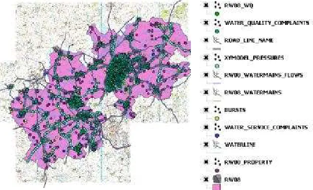
Data was provided by the water industry partner for a specific region: a production water supply zone containing a mix of urban and rural areas for a town with approximately 5000 customers (see figure 1). The area was chosen due to good data availability and suspected previous issues with stagnation. It is supplied with a chloraminated surface water source. The following data was obtained for the case study for an eight year period: regulatory water quality (spot sampling with sparse temporal and spatial resolution such as iron, manganese, pH, turbidity, temperature, conductivity, total chlorine); GIS asset data (such as pipe material, diameter, length) and connectivity; customer water quality and water service contacts; hydraulic model information such as maximum velocity and water age and turbidity / iron / manganese failures.

After preliminary data exploration some of the following problems were identified: • Inconsistent data / lack of uniform referencing between differing data sets • Sparse data sampling rate for regulatory data

• Potential errors in the data

• Limited information on service pipes connections may prevent analysis of findings • Rezoning year on year

These issues are typical of all UK water service providers and more generally for most large, lengthy period, disparate datasets. The data analysis techniques employed in the study were selected to try and address such issues as far as possible.

Figure 1. Case study area

METHODS

Feature selection

was used in ArcGIS to associate the nearest pipeline to a sample (proximity search) and then collate this data into a table. A total of over 9000 unique sample records were available from the original thematic layer, covering an eight year period and with theoretically many possible fields (>150). However, in practice many of these fields were specific to the corporate database, empty, or repeated information. Some variables were considered but not included for analysis generally due to being exceedingly sparse. The most promising fields were selected as set out in Table 1, along with fields indicated from asset records and modelled data (which was obtained and linked between datasets). In Table 1, ‘condition code’ is a value between 1 and 5, (local) residence time was calculated directly using (absolute) velocity and length for each pipe and water age is the cumulative local residence time from point of entry.

Table 1. Variables incorporated in SOM analysis

Variable Type Units

Turbidity Water quality FTU Iron Water quality mg/L Temperature Water quality deg C Free Chlorine Water quality mg/L Total Chlorine Water quality mg/L Manganese Water quality mg/L Conductivity Water quality S/m Nitrite Water quality mg/L Nitrate Water quality mg/L Month/Year Water quality N/A

Variable Type Units

Length Asset m

Iron Asset mg/L

Condition code Asset N/A

Material Asset N/A

Velocity Modelled m/s

Residence time Modelled Seconds Water Age Modelled Hours Urban / Rural GIS derived N/A

These fields were imported into MATLAB either as numeric data or strings depending on the variable. For the main analysis the data was considered as 1) explanatory asset information, 2) stagnation effect or 3) explanatory cause and/or effect of stagnation.

Data preprocessing

A number of programmatic stages to deal with the variable types in an appropriate manner were required:

• Data cleaning

Scanning the data and dealing with issues such as missing data or null fields • Outlier removal

The raw data often has quite significant outliers. This is a typical problem with extracts from corporate databases and may manifest as impossibly large values for variables, or negative error codes such as -99. A degree of pre-processing is required to ‘clean’ any data sets used. In this case, as well as processing for error codes (conversion to NaNs) outliers were removed using the Thompson Tau method [9] which utilises Maximum Likelihood Estimation with an alternative outlier model.

• Data transformation and normalisation

SOM analysis

The SOM for the training vectors was generated using the program MATLAB (Version 7.2.0.635; The Mathworks Inc.) using the SOM toolbox developed at the Helsinki University of technology (available online at http://www.cis.hut.fi/projects/somtoolbox). The input layer consisted of a number of neurons corresponding to the number of variables used and the output layer consisted of a hexagonal Kohonen map whose size was optimally selected by the SOM toolbox. A batch training method was used with a Gaussian neighbourhood. The initial learning rate of 0.5 was used for the first rough phase of training corresponding to the creation of a ‘coarse’ mapping which is when the global order is imposed on the map. Later the learning rate is reduced to 0.05 for the second phase, in which the fine structure is added to the map while preserving the global order. A trained network can be labelled in a manner described by Kohonen. Each output neuron is tested against a set of inputs of some known classification. For each set, consisting of an input of each class, the distances between the weights of that neuron and the inputs are calculated and the class corresponding to the closest input is noted. A majority verdict over all the sets (using a voting approach) then determines a nodes class label, with a draw resulting in a node remaining unclassified.

RESULTS AND DISCUSSION

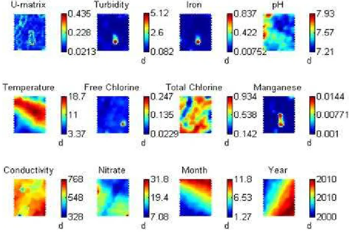
Base water quality sampling

Firstly, the regulatory data only was used to check the base water quality relationships. Figure 2 shows the resulting final Kohenen SOM map (here a 32 x 21 hexagonal map). This map contains color coded hexagons that summarize all of the component planes that represent individual variables. There are two separate parts of the SOM display. These are the summary U-matrix and the component planes for each individual variable. The U-matrix allows examination of the overall cluster patterns in the input data set after the model has been trained. Each hexagonal cell represents individual neurons, which are the mathematical linkages between the input and output layers. In the component planes for individual variables, the coloring corresponds to actual numerical values for the input variables that are referenced in the scale bars adjacent to each plot. Blue shades show low values and red corresponds to high values. Visual inspection of the component planes allows examination of how variables vary against each other. A temporal aspect was included by incorporating the month (with 1 as January to 12 as December) and year (of the sampling). We can immediately see how the temperature measurement band relates to the summer months, but there are also some other interesting factors revealed such as nitrate values being lower during later months of the year. We can also see that when turbidity is high, iron and manganese are also generally high.

Incorporating asset information with water quality and using rural/ urban labelling

labelled map, that rural areas generally appear to have lower total chlorine, and that the stagnation surrogates (Iron, manganese and turbidity) appear to have extreme values predominantly here.

Further analysis including modelled data with material labelling

A dataset derived from hydraulic modelling results was provided for further analysis, including velocities, a calculated residence time and a water age for 3240 records. It would be expected that high water age would correspond to water quality stagnation. The analysis supported this assumption, with high age being strongly correlated to increased concentrations of iron, manganese, turbidity and nitrite (see Figure 4). The final SOM uses material of pipes for labelling, which are classified by name type. Of the 11 sorts of material in the database only the following are considered (accounting for over 99% of assets): CI (C), DI (D), HPPE/PE100 (H), MDPE /PE80 (M), PVCu (P) ST (ST). Figure 4 provides the results for the labelled map using the above material codes – bottom right hand corner with colors as follows: Orange = Cast Iron, Yellow = Ductile Iron, Blue = MDPE/HPPE/PVC, Light blue= Unclassified/Other. We can immediately see strong clustering of material types and we can relate this to areas of component planes in figure 4. For example, the plastic pipes generally have a low value of condition code, low values of conductivity seem to be associated with ductile iron and as we would expect the clusters of high turbidity, iron and manganese correspond to cast iron pipes. More complex relationships can be gleaned as well, such as cast iron pipes with medium diameters and a long residence time correlate to increased levels of iron, turbidity and manganese and lower chlorine.

Figure 3. SOM results for water quality, asset, modelled data and urban/rural label

CONCLUSIONS

This study has demonstrated the application of advanced techniques to perform highly novel analysis and interpretation of complex, diverse and variable quality data from water company databases. The ability of SOMs for data mining large, multi-dimensional data sets, including the integration of heterogeneous data types across multiple databases, was utilized to identify relationships between water quality, modeled and asset data. They offer a useful synthesis and higher-fidelity visualization and hence understanding of data which is otherwise impossible for humans to grasp. A key finding from the data analysis is that the risk for water quality stagnation, for this region, appears to be greatest in cast iron pipes with medium diameters, medium to high residence times, high water age, high condition code and located in rural areas. Samples with iron failures are often associated with lower chlorine residuals and/or indicators of nitrification like nitrite. The benefit of this work is an improved understanding of water quality in stagnant zones to enable the production of robust risk assessment. Ultimately this will help deliver improved levels of service, water quality compliance and fewer customer contacts and to achieve the optimum use of resources through better stagnation flushing procedures.

Acknowledgements

The authors are grateful for the support of Anglian Water and their permission to publish the details included herein. This work was also part supported by the Pipe Dreams project (EP/G029946/1), funded by the UK Science and Engineering Research Council.

REFERENCES

[1] Geldreich, E. E., Microbial quality of water supply in distribution systems. CRC, (1996). [2] EPA, “Distribution system indicators of drinking water quality.”

http://www.epa.gov/safewater/disinfection/tcr/index.html, (2006).

[3] Carter, J. T., Lee, Y. and Buchberger, S. G.,”Correlation between travel time and water quality in a deadend loop”. Proc.Water Quality Technology Conference. Am. Wat. Wks Assoc., November 9-12, Denver, Co, USA, (1997).

[4] Unwin, D., M., Saul A., J. and Boxall J., B., “Data mining and relationship analysis of Water Distribution System Databases for improved understanding of operations performance”. In CCWI Advances in Water Supply Management, London, (2003). [5] Wu, W., Dandy, G. C. and Maier, H. R., “Protocol for developing ANN models and its

application to the assessment of the quality of the ANN model development process in drinking water quality modelling”. Environmental Modelling & Software, Vol. 54, (2014), pp 108-127.

[6] Kohonen, T.,”The Self-Organizing Map,” Proceedings of the IEEE, Vol.78, No.9, (1990), pp 1464-1480.

[7] Kalteh, A. M., Hjorth, P. and Berndsson, R., “Review of the self-organizing map (SOM) approach in water resources: Analysis, modelling and application”, Environmental Modelling and Software, Vol. 23, (2008), pp 835-845.

[8] Mounce, S. R., Douterelo, I., Sharpe, R. and Boxall, J. B.,“A bio-hydroinformatics application of self-organizing map neural networks for assessing microbial and physico-chemical water quality in distribution systems”. Proceedings of 10th International Conference on Hydroinformatics, Hamburg, Germany, (2012).