BOUT++ : Recent and current developments

This is a repository copy of

BOUT++ : Recent and current developments

.

White Rose Research Online URL for this paper:

http://eprints.whiterose.ac.uk/105679/

Version: Accepted Version

Article:

Dudson, Benjamin Daniel orcid.org/0000-0002-0094-4867, Allen, Andrew Robert,

Breyiannis, George et al. (12 more authors) (2015) BOUT++ : Recent and current

developments. Journal of Plasma Physics. ISSN 1469-7807

https://doi.org/10.1017/S0022377814000816

[email protected] https://eprints.whiterose.ac.uk/ Reuse

Items deposited in White Rose Research Online are protected by copyright, with all rights reserved unless indicated otherwise. They may be downloaded and/or printed for private study, or other acts as permitted by national copyright laws. The publisher or other rights holders may allow further reproduction and re-use of the full text version. This is indicated by the licence information on the White Rose Research Online record for the item.

Takedown

If you consider content in White Rose Research Online to be in breach of UK law, please notify us by

BOUT++: Recent and current developments

B. D. D u d s o n

†

, A. A l l e n

, G. B r e y i a n n i s

, E. B r u g g e r

,

J. B u c h a n a n

, L. E a s y

, S. F a r l e y

, I. J o s e p h

, M. K i m

,

A. D. M c G a n n

, J. T. O m o t a n i

, M. V. U m a n s k y

,

N. R. W a l k d e n

, T. X i a

, X. Q. X u

1

York Plasma Institute, Department of Physics, University of York, Heslington, York, YO10 5DD, UK

2

Japan Atomic Energy Agency, Rokkasho Fusion Institute, Rokkasho-mura, 039-3212, Japan

3

Lawrence Livermore National Laboratory, Livermore, CA 94551, USA

4

CCFE, Culham Science Centre, Abingdon, OX14 3DB, UK

5

Mathematics Department, Illinois Institute of Technology, Chicago, IL 60616, USA

6

Department of Physics, POSTECH, Pohang, Gyeongbuk 790-784, Korea

7

Institute of Plasma Physics, Chinese Academy of Sciences, Hefei, China

(Received 19 August 2014)

BOUT++ is a 3D nonlinear finite-difference plasma simulation code, capable of solving quite general systems of Partial Differential Equations (PDEs), but targeted particularly on studies of the edge region of tokamak plasmas. BOUT++ is publicly available, and has been adopted by a growing number of researchers worldwide. Here we present im-provements which have been made to the code since its original release, both in terms of structure and its capabilities. Some recent applications of these methods are reviewed, and areas of active development are discussed. We also present algorithms and tools which have been developed to enable creation of inputs from analytic expressions and experimental data, and for processing and visualisation of output results. This includes a new toolHypnotoadfor the creation of meshes from experimental equilibria.

Algorithms have been implemented in BOUT++ to solve a range of linear algebraic problems encountered in the simulation of reduced Magnetohydrodynamics (MHD) and gyro-fluid models: A preconditioning scheme is presented which enables the plasma po-tential to be calculated efficiently using iterative methods supplied by the PETSc library (the Portable, Extensible Toolkit for Scientific Computation) (Balayet al.2014), with-out invoking the Boussinesq approximation. Scaling studies are also performed of a linear solver used as part of physics-based preconditioning to accelerate the convergence of im-plicit time-integration schemes.

1. Introduction

The edge region of tokamak plasmas (Wesson 1997; Stangeby 2000) is of crucial im-portance to their feasibility and economic viability as fusion reactors. It is the interface between the hot (∼1−10 keV), fully ionised core required for fusion, and the plasma facing material surfaces which must remain cool (<1eV) to avoid excessive damage or sputtering of impurities, which could contaminate the core plasma. The wide range of temperatures and hence collisionality regimes; nonlinear plasma dynamics; atomic ionisa-tion, charge-exchange and recombination processes; impurities; and interaction with ma-terial surfaces, make modelling the plasma edge challenging. This is further complicated

by the magnetic geometry, which is usually arranged into an ’X-point’ configuration, in which the closed magnetic surfaces of the core are surrounded by open magnetic field-lines, which transport energy and particles leaving the core away into divertor regions designed to handle high heat fluxes.

Simulations of the edge of tokamaks which include many of the important atomic and impurity radiation processes are routinely performed using 1-D (Goswami et al. 2001; Fundamenskiet al.2001; Nakamura 2011) and 2-D (Rognlienet al.1992; Schneideret al.

2006; Kawashimaet al.2006) codes. These however cannot correctly predict the plasma transport across the magnetic field, which is usually anomalous (turbulent) (D’Ippolito

et al.2011), and for which diffusion (Fick’s law) is a poor approximation (Garciaet al.

2007; Naulinet al.2007; Gendrihet al.2012). The need for a first-principles understand-ing of cross-field transport in the edge region has received increasunderstand-ing attention in recent years, and several new 3-D codes have been developed to study edge turbulence (Ricci

et al. 2012; Ricci & Rogers 2013; Tamain et al. 2010). As discussed above, the

struc-ture and dynamics of the edge region of tokamaks involves a complicated interaction between many physical processes, and as a result it is not clear a priori which model or combination of models is most appropriate. To minimise duplication of effort, there is a need for a flexible code which can be adapted to solve a range of different models, and is modular enough that it can be extended in multiple ways by a large group of users. BOUT++ (Dudson et al. 2009) is an open-source 3D nonlinear finite difference code which aims to fill that need.

BOUT++ was developed originally to study tokamak edge plasma physics (Dudson

et al. 2009), taking ideas and lessons learned from the earlier BOUT code (Xu et al.

1999, 2000; Umanskyet al.2006; Xuet al.2008). It is highly modular, operates in gen-eral curvilinear coordinates and complicated mesh topologies, and can be applied to the solution of quite general Partial Differential Equations (PDEs) in three dimensions + time. Recent applications of BOUT++ include the study of plasma transients (Edge Lo-calised Modes, ELMs) (Zohm 1996; Xuet al.2010; Xiaet al.2012; Xiet al.2013), plasma turbulence (Friedman et al. 2012), and the dynamics of isolated ‘blobs’ in 3D (Angus

et al.2012b,a; Walkdenet al.2013).

The BOUT++ distribution is publicly available on Github†, and comes with a test suite and variety of plasma physics models and examples. Some have been used to produce results published elsewhere (e.g. ELM, turbulence in the LArge Plasma Device

(Gekel-man et al. 1991), and blob models), whilst others can be used as a starting point for

new physics studies. This paper describes the 2.0 release of BOUT++, which was used as a basis for the 2013 BOUT++ workshop‡: Section 2 briefly describes modifications to the structure of BOUT++ which have been made to accommodate further develop-ment; Section 3 describes improvements and new capabilities which have been added to BOUT++ since its original release (Dudson et al. 2009). Section 4 details the de-velopment of pre- and post-processing tools for equilibrium input and visualisation. In section 5 we conclude and discuss future directions for development.

2. Code structure

The BOUT++ development community has expanded significantly following its re-lease and 2011 workshop, and with that has come the need to adopt more professional software development practices: Git¶is used for version control, along with a system of

† BOUT++ public distribution http://github.com/boutproject

‡ BOUT++ workshop 2013:http://bout2013.llnl.gov

feature branches adopted from the PETSc development group (Balayet al.1997) which is described in detail on the BOUT++ development pagek. An important addition has been a test suite which can be run quickly before changes are committed, to check that nothing obvious has been broken. This has greatly simplified the process of checking code, and has resulted in many bugs being caught before they could affect production code. The majority of these tests are not physics simulations, as these would take too long to perform and so discourage regular use. Instead, tests are designed to check individual components independently for a range of inputs and processor configurations, so that the cause of a test failure can be quickly identified.

2.1. Factory pattern

To enable BOUT++ to be extended, and new implementations of solvers for boundary and initial-value problems to be added independently, components have been refactored and organised along the Factory pattern (Gammaet al. 1995; Knepley 2012), a widely used method to separate interface from implementation. Each component of BOUT++, such as file I/O or time integration solver, has a well defined interface (in C++ a base class with virtual members). Several implementations of this interface can coexist, and the user code doesn’t depend on which implementation is used. To create a particular instance, the static member function “create” is called. For example, time-integration schemes implement the “Solver” interface, so creating a new solver is done by the following:

Solver *s = Solver::create();

so that s is a pointer (hence the *) to a Solver object. Which particular instance of Solver is created (RK4, PETSc etc.) and assigned tosis set by options stored in a tree structure, which can be set in the input file or on the command-line. By default the options section for the Solver class is called “solver”, so to choose the rk4 method on the command-line the user adds

solver:type=rk4

To allow multiple solvers with different settings to be used simultaneously, the option section can be passed during creation:

Solver *s = Solver::create(

Options::getRoot()->getSection("mysolver") );

The Options tree works in a similar manner to a file system:Options::getRoot()returns a pointer to the root (lowest level) of the options tree structure, analogous to the root “/” directory of aUnixfile system;getSection()traverses the tree by returning pointers to sub-trees, and is analogous to changing to a sub-directory using “cd mysolver”. By passing this sub-tree toSolver::create(), the result is that options for this solver will be taken from the “mysolver” section of the options tree, and can be changed independently.

This pattern enables users to experiment with different numerical methods with mini-mal changes to the program inputs. As new capabilities are added to BOUT++, such as new PDE and ODE solvers, existing models can take advantage of them without needing to modify any code, only the input settings. To the extent possible, this separation of

interface and implementation reduces the number of dependencies between parts of the code and allows researchers to benefit from each other’s work on separate components. A similar system is used by the Trilinos project (Herouxet al.2005), in which parameter lists are passed to objects on creation in order to allow changing of options at run-time.

2.2. Library interface

The interface between the core BOUT++ code and problem-specific “user” code has also been modified since the original publication. The original BOUT++ was structured as a framework so that the main() function was defined internally, and the user sup-plied two functions: one for initialisation of the desired physics model, and one which calculated the time-derivative of each evolving variable given the system state. Further callback functions were later added for optional preconditioning (section 3.3) and system Jacobian calculations. This method was simple to implement, and familiar to those with a background in C programming, but caused complications when combining BOUT++ with other libraries and frameworks. In addition to this original style, an object-oriented style is now supported: Rather than callback functions, users implement a class which in-herits fromPhysicsModel, overriding the default functions as needed. A simple example is a diffusion equation in 1-D, which could be implemented in the following code:

class Diffusion : public PhysicsModel { private:

Field3D T; protected:

void init(bool restarting) { SOLVE_FOR(T);

}

void rhs(double time) { ddt(T) = Laplace_par(T); }

};

This defines a 3D scalar field (Field3D) T; specifies that T should be evolved in the initialisation function init; and then calculates the time-derivative as ∂T

∂t = ∇ · (b0b0· ∇T) in the function rhs, in which ddt()should be read as ∂/∂t. Users can use

a macro BOUTMAINto define a standard main() function, or define their own to enable BOUT++ to be combined with other libraries. Separating physics models into classes allows the possibility of combining several models into a single simulation, for example a model for neutral gas with a plasma model, and could be exploited for multiscale simulations.

The above example illustrates some other minor improvements which have been made to BOUT++: ddt()and SOLVE FOR are preprocessor macros, which are used sparingly wherever the resulting improvement in readability outweighs their potential for causing hard-to-find bugs.

3. Solvers and capabilities

elliptic solvers for calculating the electrostatic potential φare presented in section 3.1, and an algorithm to solve parabolic equations along magnetic field lines is presented in section 3.2. This latter solver has been used as part of a physics-based precondition-ing strategy (Mousseau et al.2000; Knoll et al.2001) to improve convergence for large time steps, described in section 3.3, and to calculate closure terms for gyro-fluid opera-tors (Dimits et al.2013). Wherever possible, these new solvers have been implemented using the factory pattern (section 2.1) and a generic interface, so that they can be reused in many plasma models and geometries.

3.1. Calculation of potentialφ from vorticity

Reduced MHD models solved in BOUT++ are commonly formulated in terms of a vor-ticity equation, from which the electrostatic potential is calculated. In reduced MHD, this can be derived from either the momentum equation or charge conservation (current continuity) (Hazeltine & Meiss 2003; Catto & Simakov 2004). Gyro-fluid models, which are an area of current research in BOUT++ (Xu et al. 2013), can also be cast in a vorticity formulation (Ottaviani & Manfredi 1999), or the potential can be calculated from a polarisation equation coupling electron and ion gyro-centre densities (Beeret al.

1997; Scott 2005a). In either case, the electrostatic potentialφis calculated by solving an equation of the form:

∇ ·min

B2 ∇⊥φ

=ω (3.1)

with ion massmi, plasma densityn, and magnetic field strengthB. The time evolution of the right hand sideω (vorticity) depends on the particular model. The coefficientn/B2

arises from the ion polarisation, and in general will vary in 3D as the density n is an evolving quantity.

Elliptic equations of the same form as equation 3.1 arise in many fields, and so nu-merical methods for their solution have been extensively studied. There are therefore many different methods available in the literature (e.g. (Iserles 2009)); the challenge is in finding one which is efficient enough for practical applications. Solving forφrequires the solution of a linear (matrix) problem for every evaluation of the time-derivatives of the system, which will usually be several times per time step. A typical turbulence or ELM simulation might require 104₋₁₀6_{time steps, and so efficient solution to equation 3.1 is}

critical for the overall run-time of the simulation.

A common approximation in plasma simulations is to neglect the variation ofn/B2

in space and/or time, referred to as the Boussinesq approximation (Yu et al. 2006). BOUT++ simulations have usually replaced the full density n in equation 3.1 with the axisymmetric (constant in toroidal angle) equilibrium density n0. Since B is also

axisymmetric, the left hand side of equation 3.1 can then be Fourier transformed in toroidal angle, decoupling the toroidal harmonics. Each toroidal harmonic can then be solved efficiently as a 1D tridiagonal system of complex equations in the radial coordinate. This scheme will be referred to here as the FFT or Boussinesq method.

To remove the Boussinesq approximation, and allow the solution to the full vorticity equation, BOUT++ has been coupled to the PETSc library (Balay et al. 1997, 2010, 2014). Here we present details of the numerical scheme, and leave exploration of the impact on simulations of plasma phenomena to a future publication.

3.1.1. Iterative solution with PETSc

By discretising equation 3.1, the calculation ofφfromωcan be cast as a linear algebra problem of the form

Ax=b (3.2)

In BOUT++ this discretisation is done by Finite Differences, but other choices such as Finite Element are used elsewhere. The resulting matrix can then be solved using the Krylov subspace (KSP) iterative solvers available in PETSc, such as GMRES. Itera-tive methods are attracItera-tive because they have smaller memory requirements than direct solvers, as Aneed never be explicitly stored, and in principle iterative methods can be parallelised more efficiently.

In general, equation 3.1 will couple all points in the domain, so theN×Nsparse matrix has a size N ≃106_{. By neglecting derivatives parallel to the magnetic field, which are}

assumed small in drift-ordered fluid (Hazeltine & Meiss 2003) and gyro-fluid (Ottaviani & Manfredi 1999) models, this can be simplified to solving multiple independent N ≃

104 _{matrices. Since the density n is evolving in time, the coefficients in this matrix}

change every time step. This makes direct solution methods based on matrix factorisation inefficient, as the matrix must be frequently re-calculated and re-factored. It is for this reason that iterative methods have been implemented in BOUT++, as these do not require the explicit calculation of the matrix elements or costly matrix factorisations.

3.1.2. Preconditioning of iterative solver

When solving large and/or ill-conditioned problems, iterative solvers can fail to con-verge, or converge very slowly after a small number of iterations (referred to as stalling). To accelerate convergence, an approximate solver is often used to “precondition” the problem, improving the condition of the matrix which the iterative solver is inverting. See for example (Golub & Van Loan 2013). A preconditionerP is an approximate in-verse of A, which needs to be calculated quickly for the overall scheme to be efficient. The equation above can be multiplied through byP as aleft preconditioner:

(PA)x=Pb (3.3)

or as a right preconditioner:

(AP) P−1 x

=b (3.4)

and this modified system is solved using the iterative method. In the limit that the preconditioner P is the inverse of A, PA is the identity, and no iterations should be required.

To test preconditioning methods, a 2D (x,z) test case was used with a density profile of the form:

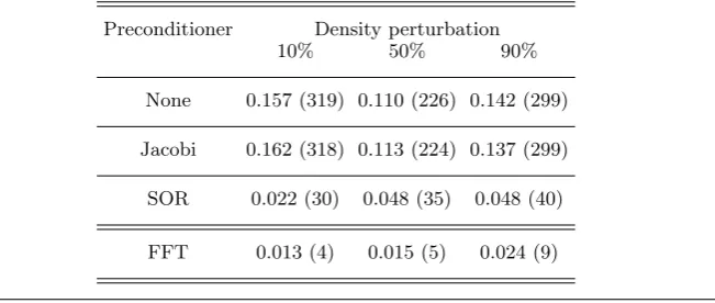
Table 1.Timing for solution on a 40×32 mesh. Shown are the wall clock times in seconds, and the iteration counts in brackets

Preconditioner Density perturbation

10% 50% 90%

None 0.157 (319) 0.110 (226) 0.142 (299)

Jacobi 0.162 (318) 0.113 (224) 0.137 (299)

SOR 0.022 (30) 0.048 (35) 0.048 (40)

FFT 0.013 (4) 0.015 (5) 0.024 (9)

the iteration count in brackets for a single solve, as the perturbation size is increased from 10% to 90% (i.e.pvaries from 0.1 to 0.9). Without preconditioning the iterative method requires ≃300 iterations and ≃1.5 seconds to converge, compared to a time of ≃2ms for a single Boussinesq solve. To improve on this, several “black box” preconditioning schemes are available in PETSc, such as Jacobi iteration or Successive Over Relaxation (SOR) methods (Iserles 2009). These methods are not problem specific, and so require only a run-time switch to enable and configure. For the problems tested, the SOR method reduced the run-time (see table 1), but the number of iterations remained prohibitive. To improve on these, a problem-specific preconditioner has been implemented.

As discussed above, the purpose of a preconditioner is to quickly find an approximate inverse to the linear problem (matrixAabove). The Boussinesq FFT-based solver is just such a solver, as it finds a fast solution by simplifying the coefficients. We therefore use the FFT solver as a preconditioner for the full problem, by wrapping the FFT solver in a PETSc PCShell preconditioner object which is then passed to PETSc to be used in the iterative solver. This preconditioner is extremely good when the density perturbation is small, but we should expect it to become less effective as the size of the density perturba-tion becomes large. This is what is observed in Table 1: For small perturbaperturba-tions (10%), the run-time is a little over half that of the SOR method, but as the density perturbation amplitude increases so does the iteration count and run-time for all methods. Even at 90% density perturbation, however, this preconditioner is still highly effective. Based on this small test, a larger study was performed to compare the SOR and FFT (Boussinesq) preconditioners.

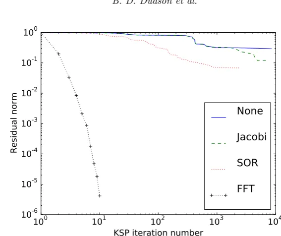
For a 516×256 mesh more typical of ELM and turbulence calculations, the iterative solver will typically stall without good preconditioning, as shown in figure 1. Using a 90% density perturbation (reducing the accuracy of the FFT preconditioner), and using the FFT solver result as the starting point for the iterative solver gives the convergence shown in figure 1. Without preconditioning, or using Jacobi or SOR preconditioners, the residual is only reduced by a factor of 10 in nearly 104 _{iterations; using the}

FFT-based preconditioner the residual is reduced by a factor of≃105 _{in 10 iterations. This}

10

₁₀

₁₀

₁₀

₁₀

KSP iteration number

10

10

10

10

10

10

10

Residual norm

None

Jacobi

SOR

FFT

Figure 1.Iterative KSP solver residual, as a function of iteration number. Solving elliptic equation 3.1 on a 516×256 mesh.

3.2. Parabolic solver along magnetic field-lines

In the reduced MHD and gyro-fluid models which BOUT++ specialises in solving, the magnetosonic fast wave is removed analytically, and so the fastest physical processes are usually the shear Alfv´en wave and heat conduction along (parallel to) magnetic field-lines. Preconditioning of either of these processes for implicit time integration (see section 3.3) requires the solution to a parabolic equation of the form (Chac´onet al.2002)

A+B∂2

||0

x=b (3.6)

where ∂||0 = b0 · ∇ is the derivative along the equilibrium magnetic field b0. Even

though equation 3.6 appears to be a one-dimensional problem, due to the structure of the equilibrium magnetic field, it is in general a two-dimensional problem: The equilibrium magnetic field in a tokamak is helical, and lies on nested toroidal surfaces. If the pitch angle of the magnetic field is such that it makes an irrational number of poloidal to toroidal turns, then a single field-line will fill the 2D surface.

If magnetic perturbations were included, so that ∂2

||0 became ∂ 2

|| = (b· ∇)

2

in equa-tion 3.6, then the magnetic field lines in general no longer lie on magnetic flux surfaces, but fill a volume. This case is of significant interest, for example in studying the transport of heat in ELM crashes and in the presence of externally applied magnetic perturbations, but solving this more general problem is left to future work.

tridi-agonal systems, this method is suitable for ditridi-agonally dominant systems. This condition is satisfied for equation 3.6 when coefficientB is negative, and coefficient A is positive definite, which is the case for all cases of interest here.

In the following we assume that the magnetic flux surface has N points in toroidal angle, andM points in poloidal angle. Firstly we exploit the toroidal symmetry of the equilibrium to decompose the problem into Fourier harmonics in toroidal angleφ. This then decomposes the problem intoN complex tridiagonal systems, one for each toroidal mode, each of sizeM. If the domain is a closed magnetic surface, then the tridiagonal systems are cyclic, with a complex phase shift between the first and last row which is determined by the pitch of the magnetic field-lines. Each of theseN systems of equations therefore has the form:

             

b0 c0 a0

a1 b1 c1

. .. . .. . ..

am−1 bm−1 cm−1 am bm cm

. .. . .. . ..

cM−1 aM−1 bM−1

             

x=b (3.7)

The domain is split between processors in the poloidal direction θ, with m rows per processor, illustrated by a horizontal line in the above equation. Within each processor the rows are eliminated, reducing the problem to two boundary equations for each processor, which forms a smaller (cyclic) tridiagonal matrix:

     

β0 γ0 α0 α1 β1 γ1

α2 β2 γ2 γ3 α3 γ3

     

χ=ξ (3.8)

where ξ and χ are the boundary values ofb and xrespectively. When solving N inde-pendent systems of equations (one for each toroidal mode), they are divided between processors, and all boundary equations for a given system are gathered onto a single processor. For example if N systems are split between 2 processors, then N/2 sets of boundary equations are gathered onto each processor. Once on a single processor, the serial Thomas algorithm (with Sherman-Morrison-Woodbury formula for cyclic tridiago-nal systems (Temperton 1975)) is used to solve for the boundary values. These are then scattered back, and substituted into the original equation to obtain the solution inside each processor’s domain.

10

₁₀

₁₀

₁₀

₁₀

Number of processors

10

10

10

10

10

Wall clock time for a single solve [s]

m=5, N=64

m=5 N=256

m=10 N=64

m=20 N=64

m=40 N=64

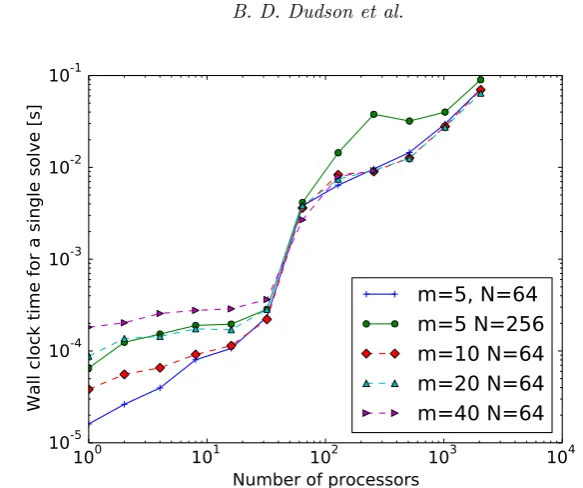
Figure 2.Soft scaling of parallel solver.mis the number of rows per processor, andN is the number of separate problems which are inverted simultaneously, corresponding to the number of toroidal Fourier modes

a node, and so becomes a bottleneck: for more than 64 processors the run time becomes almost independent of problem sizem.

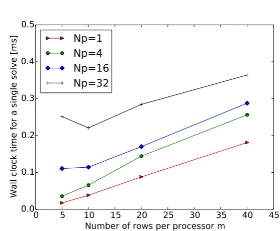
For fewer than 32 processors, it can be seen that doubling the number of independent systemsN has a similar effect to doubling the size of each systemM, and the wall time is approximately proportional to the problem size. This can also be seen in figure 3: on single core the algorithm scales approximately linearly with problem size, for larger numbers of processors there is a constant offset which depends on the number of processors, but only weakly on the number of rows per processor. The result is that as the number of rows per processormis increased, the scaling with processor number appears more favourable: In the limit that each processor only has a two rows, the algorithm becomes equivalent to gathering all rows onto one processor, and using a serial algorithm, which would result in a linear scaling with number of processorsNp. In figure 2, whenm= 5, the wall time scales withN0.77

p , whilst form= 40 the exponent is≃0.20.

0

5

10 15 20 25 30 35 40 45

Number of rows per processor m

0.0

0.1

0.2

0.3

0.4

0.5

Wall clock time for a single solve [ms]

Np=1

Np=4

Np=16

Np=32

Figure 3. Soft scaling of parallel solver showing same data as figure 2 for N = 64. Shows variation of wall-clock time with problem size per processormfor different numbers of processors

Np.

This tridiagonal solver has been used to implement physics-based preconditioning (Mousseau

et al.2000; Knoll et al.2001) in BOUT++ (Dudsonet al. 2012), which is discussed in

section 3.3. It has also been used to implement gyro-fluid parallel closures such as those due to (Hammett & Perkins 1990) by approximating to high accuracy the k/|k| using a small number of Lorentzians, which take the form of equation 3.6. This has enabled these closures to be applied in situations where Fourier methods cannot be used, such as global simulations in realistic toroidal geometry. Further details can be found in (Dimits

et al.2013; Xuet al.2013).

3.3. Time integration

The time integration schemes available in BOUT++ have been expanded to include ex-plicit schemes (RK4, Euler (Iserles 2009)), a scheme derived by Karniadakiset al (Kar-niadakis et al. 1991; Scott 2005b), and a range of implicit schemes through coupling to the SUNDIALS (SUite of Nonlinear and Differential/ALgebraic equation Solvers) ( (Hindmarshet al.2005) and PETSc (Portable, Extensible Toolkit for Scientific Com-putation) (Balayet al.1997, 2010) libraries.

The need to solve increasingly complicated models at increasingly high resolution has made efficiency and parallel scaling of algorithms used important. Plasma models are typically stiff, meaning that explicit integration methods are limited to small time-steps relative to the time-scales of interest. Implicit time integration methods overcome this restriction, but require the solution of a large linear system (N×N where N is the number of evolving variables, typically 1−10 million) at every timestep. Unless this can be done efficiently, the overall time taken by an implicit solver may not be less than an explicit solver.

time integration method is solving a nonlinear problem to find the state at the next time point. Using a scheme such as Newton’s method, this nonlinear problem is reduced to one or more steps which require the solution to a linear problem of the formAx=bwhere

bis known, and depends on current and previous state and their time-derivatives;x is related to the unknown state at the next timestep; andA is a large matrix. Advancing a single time-step therefore involves an outer loop to solve the nonlinear problem, which contains an inner loop to find the solution to a series of linear problems. Preconditioning targets this inner loop, improving convergence of the linear solve in order to reduce the overall run time.

Physics-based preconditioning describes a family of approaches to deriving precon-ditioners, which use knowledge of the physical system to simplify the model equa-tions (Mousseauet al.2000; Knollet al.2001). The aim is to retain in the preconditioner only those processes (oscillatory or diffusive) which are limiting the timestep. This then improves the condition number of the matrix which the iterative (usually Krylov sub-space) method has to solve. Because the iterative method converges towards the solution to the full system, approximations can be made in the preconditioner without affecting the final solution, only the convergence rate towards the solution. The approach we have followed is based on work by Chacon and others (Chac´on et al.2002). Preconditioning of the implicit solvers in BOUT++ (using SUNDIALS and PETSc libraries) has been implemented in BOUT++, described in (Dudsonet al. 2012).

An example is the shear Alfv´en wave which is present in all 3D turbulence models. In the simplest form of the reduced MHD equations, this wave can be described by the following coupled equations for vorticity ω (equation 3.1), and magnetic potential A|| which describes the perturbed magnetic fieldδB=∇ × b0A||

:

∂ω

∂t =∇||0 j||

∂A||

∂t =−∂||0φ (3.9) ω=∇ ·min

B2 ∇⊥φ

∇2

⊥A||=−µ0j||

where∇||0f =∇ ·(b0f),∂||0=b0· ∇,∇⊥f =∇f−b0(b0· ∇f), and∇2_⊥f =∇ ·(∇⊥f). These equations can be combined to give a wave equation, which in the case thatn/B2

is a constant reduces to:

∂2_ω ∂t2 =∇||0

∂j||

∂t =∇||0

1

µ0

∇2

⊥∂||0 B2 min

∇−2

⊥ ω

(3.10)

By further assuming that the magnetic fieldBvaries slowly, and so neglecting derivative ofB terms,

∇||0∇ 2

⊥∂||0∇− 2

⊥ ≃∂

2

||0 (3.11)

and the shear Alfv´en wave propagates only along the (equilibrium) magnetic field:

∂2_ω ∂t2 =

B2 µ0min

∂2

||0ω=V 2

A∂

2

||0ω (3.12)

whereVA is the Alfv´en speed. In tokamak simulations, this speed can beVA≃107m/s, severely restricting the time step for explicit time integration schemes. If hyperbolic equation 3.12, or the original equations 3.9 are solved implicitly, then this requires the solution to a parabolic equation. For example using a backwards Euler method:

ω ω′ t+1 = ω ω′ t +δt 0 1 V2 A∂ 2

||0 0

ω ω′

t+1

the equation to be solved at each timestep is parabolic:

1−δt2

V2

A∂

2

||0

ω

ω′

t+1

=

1 δt δtV2

A∂

2

||0 1

ω ω′

t

(3.14)

and of the same form as equation 3.6. To precondition waves of this type, the parabolic solver discussed in section 3.2 can therefore be used.

The above procedure has converted a wave equation 3.12 into a parabolic equation, so that waves which are not resolved by the time integration, for which the Courant number is greater than 1, are slowed and damped. This is an inevitable consequence of implicit time integration (Chac´on et al. 2002), rather than a property of this preconditioning scheme. Implicit time integration with preconditioning (physics-based or otherwise) is only effective if the timescales of interest are long compared with the smallest timescales in the system. This is almost always the case in simulations of tokamak plasmas, for which drift or resistive timescales of interest are usually slow compared to dynamics such as electron heat conduction and shear Alfv´en wave propagation along magnetic field-lines.

The assumptions made to reduce the full set of equations 3.9 to wave equation 3.12 cannot be made in the calculation of time-derivatives for the full problem, as this would affect the solution, but they can be made in the preconditioner since this is used to find an approximate solution to accelerate convergence to the solution of the full set of equations. The full procedure to derive a preconditioner using Schur factorisation is described in (Dudson et al. 2012), and is somewhat more involved than outlined here, but it makes the same assumptions and so results in the same form of equations. The resulting preconditioner using the solver presented in section 3.2 has been found to result in significant speed-ups for sets of equations where the timestep was limited by the shear Alfven wave and parallel heat conductivity (Dudsonet al.2012), reducing overall wall-clock time by an order of magnitude in some cases.

4. Pre- and Post-processing tools

A simulation code is of little use without the tools to create high quality inputs such as meshes, and to analyse and present the results of the simulations. For post-processing the most important requirement is to be able to read the simulation output data in the user’s language of choice. Routines to do this are now available for IDL†, Python, Matlab, Octave, and Mathematica (Wolfram Research, Inc. 2014) as part of the public BOUT++ repository.

For most publications, 1D plots and 2D contours are sufficient, but there are occasions when the ability to visualise data in three dimensions is useful. In the early stages of a scientific investigation, seeing the entire simulation domain rather than slices through it, can help spot anomalies or unexpected features. When presenting results, particularly at conferences, 3-D visualisation can quickly convey a large amount of information. Wrap-pers have been developed to enable two scientific data visualisation packages to be used with BOUT++: Mayavi‡and VisIT¶.

Tools have also been developed to enable more convenient input of initial profiles and sources (section 4.1), and processing of experimental equilibria into input meshes (section 4.2).

† IDL: http://www.exelisvis.co.uk/ProductsServices/IDL.aspx

‡ Mayavi project,http://code.enthought.com/projects/mayavi/

×

sin()

−

z

×

3 y

· · ·

Figure 4.A tree of generator objects (Abstract Syntax Tree) to evaluate the expression (...)*sin(3*y-z)

4.1. Input expression parser

Many simulations do not require complex geometry, but are intended to study basic phys-ical mechanisms in slab or cylindrphys-ical geometries. For these cases the initial conditions and parameters often follow analytic expressions. If these expressions can be stored in the input files rather than preprocessing scripts, then inputs can be modified more quickly, and a clearer record of simulation inputs is kept for later reference. Examples include 2D blob simulations, where the initial density profile is a Gaussian inxspecified using:

function = 1 + 0.2*gauss(x-0.25, 0.1)

In slab simulations of forced reconnection, a helical external magnetic potential is applied to an initial sheared magnetic field. This external field can be specified in the input file using:

function = (1-4*x*(1-x))*sin(3*y - z)

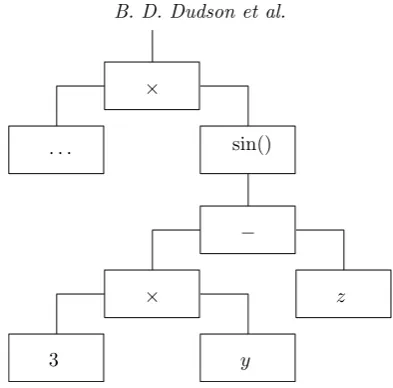
A recursive descent parser with operator precedence (see e.g.(Ahoet al.2006; LLVM Project 2014)) is used to build an Abstract Syntax Tree (AST) of generator objects from the input text: A constant generator like ’3’ or ’pi’ always returns the same value; a coordinate generator like ’x’ returns a value depending on the cell location; and a binary operation generator like ’+’ or ’sin’ depends on the value of its children generators. Part of the AST for the above example is shown in figure 4. This tree is then evaluated for each cell in the domain to obtain the required initial conditions. This method is not computationally efficient, but is only used during initialisation and provides the flexibility to adapt the code in future.

and boundary conditions need to be specified. This verification activity is ongoing, and will be presented in a future publication.

As demonstrated by libraries such as SciPy (Joneset al.2001–), the combination of an efficient statically compiled library with the flexibility of an run-time interpreter can be very powerful. A possibility for future exploration is to use a scripting language such as Python, Lua, or Scheme to provide input and output to BOUT++, or even to implement parts of physics modules. These languages provide a complete programming environment, but would require significant work to interface with the C++ classes in BOUT++.

4.2. Mesh generation

The accuracy and robustness of plasma simulations is strongly dependent on the quality of the input mesh: noise in the metric components, or large variations in the grid spacing leads to noise in the solution, restrictions in the timestep, and occasionally numerical instabilities.

Generating meshes for tokamak equilibria with X-points is challenging due to the change in topology across the separatrix, the shape of the boundary around the plasma, and the variation in geometry between machines. The original BOUT code used UEDGE

(Rogn-lienet al.1992, 2002) to generate grids, and BOUT++ can also use these input files with

a little preprocessing. There are several other tools available for generating these meshes such as CARRE (Marchand & Dumberry 1996), but none are open-source licensed and suitable for distribution with BOUT++.

To generate X-point meshes for BOUT++ from experimental free boundary equilibria, a new code named Hypnotoadhas been developed, and is available in the BOUT++ public repository. The main features of this grid generator are that it:

(a) Was originally written entirely in IDL. This allows Hypnotoad to be run anywhere where IDL is available, without the need for a compilation step and complicated depen-dencies. IDL is widely available and used in fusion research institutions, and comes with a large library of built-in functions. Work is currently ongoing to port the algorithms which have been developed into Python, and indeed many of the figures shown here will be from the Python version, due to the superior graphical capabilities of the Python library Matplotlib†.

(b) Automatically adjusts settings when needed. The grid produced can be customised, but the minimum number of inputs is very small (number of grid points and a range of poloidal flux ψ). The ψ range asked for is adjusted to fit within the boundary, with configurable levels of strictness.

(c) Can handle an arbitrary number of X-points. Whilst not of obvious benefit since most tokamak equilibria are single or double-null, this means thatHypnotoadis quite generalised and can cope with unusual configurations. It has been applied to Snowflake-like configurations (Maet al.2014), but only in snowflake-plus configurations where the second X-point was not included in the mesh.

Because this grid generator is intended to be used for many different tokamaks, robust algorithms have been developed which can handle the large number of possible configu-rations encountered. To date, this grid generator has been successfully used to generate meshes from C-MOD, DIII-D, EAST, ITER, JET, MAST and NSTX tokamak equilib-ria (Wesson 1997), without requiring any machine-specific alterations or inputs beyond the EFIT generated G-EQDSK or ’g’ file (Laoet al.1985, 2005; General Atomics 2014). The production of a BOUT++ input mesh consists of three stages: Analysis of the equilibrium to determine X-point locations, construction of mesh points, and calculation

0.0 0.5 1.0 1.5 2.0 2

1 0 1 2

0

0

1 1

2 2

3 4

5 3 6 7

4

8

-0 .0 00 80

3

Major radius [m]

He

igh

t

[m

]

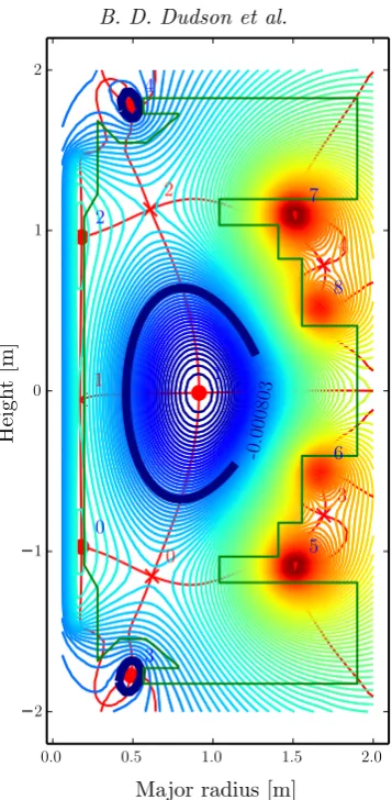
Figure 5.Automated identification of O- and X-points in a MAST double-null configuration

of metric tensor and equilibrium quantities. The key features and algorithms used in each of these stages are described in the following sections.

4.2.1. Finding X-points

The first task in generating a mesh is to determine the number and location of the O- and X-points of the plasma. These correspond to critical points (maxima, minima, or saddle points) of the poloidal flux functionψ(R, Z), which for tokamak equilibria is a 2D function of major radiusRand heightZ. The most robust technique for finding these has been found empirically to be to produce contour lines ofdψ_dR = 0 and dψ_dZ = 0. Intersections of these lines then give locations of critical points. By comparing second derivatives ofψ

at these critical points it can be determined whether they are O-points (minima/maxima) or X-points (saddle points). An example of a double-null equilibrium from the Mega-Amp Sherical Tokamak (MAST) is shown in figure 5. Contours of dψ

dZ = 0 and dψ

Major radius [m]

He

igh

t

[m

]

Major radius [m] a)

b)

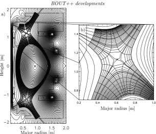
Figure 6.Mesh produced for MAST double-null equilibrium (shot 14220)

When the boundary shape is specified, critical points close to the poloidal field coils can be discarded as being outside the boundary, though ripples in the solution due to the central solenoid at major radiusR= 0 can lead to spurious O- and X-points on the inboard side: In figure 5 two O-points (labelled ’0’ and ’2’), and one X-point (labelled ’1’) can be seen close to the centre column. These can usually be excluded through choice of

ψrange or boundary contour. 4.2.2. Meshing

Transport of heat and particles in magnetised plasmas are strongly anisotropic, and as a result fluid simulations commonly use meshes aligned with magnetic flux surfaces, in order to minimise mixing the directions perpendicular and parallel to the magnetic field. The coordinates currently used by BOUT++ for tokamak simulations are orthogonal in the poloidal (R-Z) plane, illustrated in figure 6 for a typical MAST double-null discharge. A region close to the X-point is shown enlarged, showing coordinate lines passing around the X-point, but leaving a hole at the null itself. The mesh has a branch-cut around the magnetic X-point, which must be treated carefully to avoid creating large variations in mesh spacing, which could lead to poor numerical behavior.

Solver for Ordinary Differential Equations) algorithm (Hindmarsh 1983; Radhakrishnan & Hindmarsh 1993) through IDL or SciPy, to construct the mesh points for each value ofθ. This is then repeated for eachθcoordinate to construct a 2D mesh. Once the mesh points have been found, the metric tensor and equilibrium components are calculated.

4.2.3. Calculating metric components

Experimental equilibria are often of low resolution (65×65 is the standard EFIT output for many tokamaks), and once the pressureP and magnetic fieldBis interpolated onto a new mesh there is no guarantee that the new values will still obey ideal MHD force balance (∇ ×B)×B=µ0∇P. Ideal MHD force balance may not be an equilibrium solution to

the plasma model being simulated, but is almost invariably a good approximation, and it is important that the mesh generation process does not lead to artefacts or sources of numerical noise and instability. Care is therefore taken to ensure the accuracy and smoothness of the interpolated solution, and quantities such as parallel current density

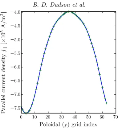
J|| are calculated multiple ways and compared as a consistency check. The interpolation method used can have a significant impact on the quality of the results: many terms such as the curvature and parallel current involve second derivatives of equilibrium flux, and these quantities should themselves be smoothly varying inputs to the simulation.

As discussed elsewhere (Xuet al.2008; Dudsonet al.2009), in order to efficiently simu-late structures (predominantly) aligned to the magnetic field, BOUT++ uses grid-points placed in a field-aligned coordinate system. From the standard, orthogonal, toroidal co-ordinate system (ψ, θ, ζ) new coordinates (x, y, z):

x=σBθ(ψ−ψ0) y=θ (4.1) z=σBθ ζ−

Z θ

θ0

ν(ψ, θ)dθ

!

whereσBθ ≡Bθ/|Bθ|is the sign of the poloidal field, and ν is the local field-line pitch given by

ν(ψ, θ) =B· ∇ζ

B· ∇θ = Bζhθ

BθR

(4.2)

where Bζ is the toroidal magnetic field, Bθ the poloidal magnetic field,R is the major radius, andhθis poloidal arc length divided by 2π. In the limit of a circular cross-section equilibrium, hθ becomes the minor radius r. The coordinate system is chosen so thatx increases radially outwards, from plasma to the wall. The sign of the toroidal field Bζ can then be either positive or negative.

By equating contravariant x components of J×B = ∇P, radial force balance in field-aligned coordinates can be written as:

∂ ∂x

_B2_h

θ

Bθ

−BζR

∂ ∂x

_B

ζhθ

RBθ

+µ0hθ

Bθ

∂P

∂x = 0 (4.3)

Close to the X-points, Bθ →0 and the above expression becomes singular, so a better way to write this is:

∂ ∂x B

2

hθ−hθBθ

∂Bθ

∂x

−BζR

∂ ∂x

_B

ζhθ

R

+µ0hθ

∂P

∂x = 0 (4.4)

This expression is used to calculate the pressure, by integrating ∂P

Radial index

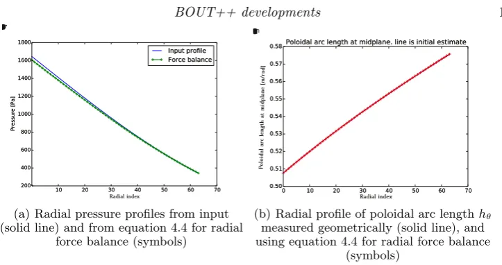
(a) Radial pressure profiles from input (solid line) and from equation 4.4 for radial

force balance (symbols)

Radial index Po loi da la rc len

gthat

mi dp lan e[ m/ra d]

(b) Radial profile of poloidal arc lengthhθ measured geometrically (solid line), and using equation 4.4 for radial force balance

(symbols)

Figure 7.Comparison of pressure andhθ profiles calculated using radial force balance (equation 4.4) with a reference calculated independently.

and compared with the values calculated from geometric arc-length. An example result of this comparison is shown in figure 7. In figure 7(a) the pressure at the outermost radial point has been set to the value from the EFIT input, and then integrated inwards according to equation 4.4. In figure 7(b) the pressure gradient from EFIT has been used, and equation 4.4 solved for hθ. Both show good agreement, indicating that the mesh generation is sufficiently accurate and smooth to retain radial force balance. This is not always observed, and where large discrepancies are observed the equilibrium should not be used.

Many reduced MHD models make use of the quantity

B

2∇ ×

_b

B

≃b×κ (4.5)

where κ = b· ∇bis the curvature vector, which arises from magnetic particle drifts. Calculation of this quantity involves second derivatives of the input poloidal fluxψ, and so must be calculated carefully to avoid introducing noise. Several methods have been tried, including:

(a) Calculate curvature on the original R-Z mesh supplied as input, then interpolate onto the new field-aligned mesh. This has been found to usually produce the smoothest result and so is the default. Using DCTs to calculate differentials of the magnetic field components was found to produce oscillatory results, so a 3-point Lagrangian interpola-tion is used instead.

(b) Calculate curvature on the field-aligned mesh in toroidal coordinates, using nearest neighbours and least-square fitting.

(c) Calculate curvature in field-aligned coordinates using

∇ ×

_b

B

= Bθ

hθ _∂ ∂x _h θ Bθ − ∂ ∂y _σ

BθBζIR

B2 ez + ∂ ∂y _σ

BθBζR

B2 ex + ∂ ∂x

σBθBζR

B2

ey

0 10 20 30 40 50 60 70 7

.5 7

.0 6

.5 6

.0 5.5 5

.0 4

.5 4

.0

P

ar

al

le

l

cu

rr

en

t

d

en

si

ty

j||

[

×

10

5

A/m

2]

Poloidal (y) grid index

Figure 8.Comparison ofj||from input profiles (equation 4.8) and divergence of current

(equation 4.7)

Methods (b) and (c) are based on calculating differentials on the output (field-aligned) mesh. They work well when the input is of high resolution, but become noisy once the resolution of the output grid significantly exceeds that of the input. Since high resolutions are required for BOUT++ simulations, this is nearly always the case, and so method (a) is preferred. Methods (b) and (c) are retained for cross-comparison.

Finally, a cross-check is made between the parallel current and the curvature. In a tokamak equilibrium the divergence of the parallel current balances the divergence of diamagnetic current, so that the total current is divergence free. In reduced MHD models this appears through the vorticity equation. The following relationship should therefore be satisfied:

∇||0j||0+∇ ×

b

B

· ∇P = 0 (4.7)

From this the parallel current can be calculated, and compared with the parallel current calculated from the inputf =RBζ and pressureP profiles:

µ0j||=−B

∂f ∂ψ −µ0

f B

∂P

∂ψ (4.8)

For the MAST equilibrium shown in figure 6 and figure 7 the parallel current calcu-lated from the curvature and pressure gradient (equation 4.7) is shown in figure 8, and compared to the current given by equation 4.8.

5. Conclusions

Recent improvements to the BOUT++ simulation framework have been summarised. Since its original release (Dudsonet al.2009), BOUT++ has been adopted by a growing number of users, who have extended its capabilities in a number of ways: the structure of the code has been improved; more complex elliptic and parabolic equations can be solved, through coupling to the PETSc library and built-in implementations; the input and output tools have been improved to enable experimental or theoretical equilibria and profiles to be imported into BOUT++.

A preconditioning scheme has been presented which enables simulations to be per-formed without invoking the Boussinesq approximation in the vorticity. This method can now be used to perform more accurate simulations of tokamak edge turbulence and Edge Localised Modes (ELMs) (Zohm 1996), the exploration of which is the subject of future work. More general elliptic and parabolic solvers for preconditioning and vortic-ity inversion problems in 3D are currently under development, and will be presented elsewhere.

Soft scaling studies have been performed for a parabolic solver along equilibrium field-lines. We find that although the scaling with problem size is good (being based on the O(n) serial Thomas algorithm), the scaling with processor number is quite poor due to the global gather and scatter operations used. Improving this will be a subject of future work.

The use of software development practices such as version control with Git and au-tomated testing has been described. A more rigorous set of tests using the Method of Manufactured Solutions (Roache 1998; Salari & Knupp 2000) for code verification are currently under development, and will be described elsewhere.

In addition to the improvements described herein, significant progress has also been made in improving the calculation of heat fluxes along magnetic field-lines, which are of-ten poorly described by the Spitzer formula (Wesson 1997) or limiter schemes (Schneider

et al. 2006; Tskhakaya 2012; Tskhakaya et al. 2008): An extension of the

Hammett-Perkins model to non-Fourier methods (Dimitset al.2013), and a method based on solv-ing a 1-D time-independent kinetic equation along magnetic field-lines (Ji et al. 2009; Omotani & Dudson 2013), have both been implemented in BOUT++. Testing of these methods against kinetic simulations, primarily for simulation of transients such as ELMs, is the subject of ongoing work.

Acknowledgements

This work was funded by EPSRC grant EP/K006940/1 using HECToR computing resources through the Plasma HEC consortium grant EP/L000237/1. EURATOM Mo-bility support is gratefully acknowledged. The views and opinions expressed herein do not necessarily reflect those of the European Commission.

REFERENCES

Aho, A V, Lam, M S, Sethi, R & Ullman, J D2006Compilers: Principles, Techniques, and

Tools. Addison-Wesley.

Angus, J R & Umansky, M V2014Physics of Plasmas 21_{, 012514.}

Angus, J R, Umansky, M V & Krasheninnikov, S I2012a3d blob modelling with bout++.

Contrib. Plasma Phys.52_{, 348–352.}

Austin, T M, Berndt, M & Moulton, J D2004 Tech.Rep. LA-UR 03-4149. LANL, USA.

Balay, Satish, Gropp, William D., McInnes, Lois Curfman & Smith, Barry F.1997

InModern Software Tools in Scientific Computing (ed. E. Arge, A. M. Bruaset & H. P.

Langtangen), pp. 163–202. Birkhauser Press.

Balay, Set al.2010Tech. Rep.ANL-95/11 - Revision 3.1. Argonne National Laboratory.

Balay, Satishet al.2014 PETSc Web page.http://www.mcs.anl.gov/petsc.

Beer, M Aet al.1997Physics of Plasmas4_{(5), 1792–1799.}

Catto, P J & Simakov, A N 2004 A drift ordered short mean free path description for magnetized plasma allowing strong spatial anisotropy.Physics of Plasmas11_{(1), pp. 90–}

102.

Chac´on, L., Knoll, D. A. & Finn, J. M.2002J. Comput. Phys.178_{(1), 15–36.}

Dimits, A M, Joseph, I & Umansky, M V2013 A fast non-Fourier method for Landau-fluid operators.Physics of Plasmas21_{(5), 055907.}

D’Ippolito, D A, Myra, J R & Zweben, S J2011Physics of Plasmas 18_{, 060501.} Dudson, B, Farley, S & Curfmann McInnes, L2012arXiv:1209.2054 .

Dudson, B Det al.2009Comp. Phys. Comm.180_{, 1467–1480.}

Friedman, B, Carter, T A, Umansky, M V, Schaffner, D & Dudson, D2012Physics of

Plasmas19_{, 102307.}

Fundamenski, Wet al.2001J. Nucl. Materials290-293_{, 593.}

Gamma, Erich, Helm, Richard, Johnson, Ralph & Vlissides, John1995Design Patterns:

Elements of Reusable Object-Oriented Software. Addison-Wesley.

Garcia, O Eet al.2007J. Nucl. Materials 363_{, 575.} Gekelman, Wet al.1991Rev. Sci. Instr.62_{, 2875.} Gendrih, Phet al.2012J. Phys.: Conf. Ser.401_{, 012007.}

General Atomics2014 G EQDSK file format. https://fusion.gat.com/theory/Efitgeqdsk.

Golub, G H & Van Loan, C F2013 Matrix Computations. The Johns Hopkins University Press.

Goswami, Ret al.2001Physics of Plasmas 8_{, 857.}

Hammett, G W & Perkins, F W1990Phys. Rev. Lett.64_{, 3019.}

Hazeltine, R D & Meiss, J D2003Plasma Confinement. Dover publications.

Heroux, M Aet al.2005ACM Trans. Math. Softw.31_{(3), 397–423.}

Hindmarsh, A C1983 InScientific Computing (ed. R. S. Stepleman et al.),IMACS

Transac-tions on Scientific Computation, vol. 1, pp. 55–64. North-Holland, Amsterdam.

Hindmarsh, A Cet al.2005 SUNDIALS: Suite of nonlinear and differential/algebraic equation solvers.ACM Transactions on Mathematical Software 31_{(3), 363–396.}

Hockney, R W1965J. Assoc. Comput. Mach.12_{, 95.}

Iserles, Areih2009A First Course in the Numerical Analysis of Differential Equations. Cam-bridge University Press, ISBN: 978-0-521-73490-5.

Ji, J Y, Held, E D & Sovinec, C R2009Physics of Plasmas16_{(2), 022312.}

Jones, Eric, Oliphant, Travis, Peterson, Pearuet al.2001– SciPy: Open source scientific tools for Python.

Karniadakis, G E, Israeli, M & Orszag, S A1991J. Comput. Phys.97_{, 414.} Kawashimaet al.2006Plasma Fusion Res.1_{, 31.}

Knepley, M G2012arXiv:1209.1711 .

Knoll, D Aet al.2001SIAM J.Sci.Comput.23_{(2), 381.}

Lao, L L, St. John, H, Stambaugh, R D, Kellman, A G & Pfeiffer, W 1985 Recon-struction of current profile parameters and plasma shapes in tokamaks.Nucl. Fusion 25_,

1611–22.

Lao, L L et al.2005 MHD equilibrium reconstruction in the DIII-D tokamak.Fusion Science

and technology 48_{, p968.}

LLVM Project2014 Implementing a language with LLVM. http://llvm.org/docs/tutorial/.

Ma, J F, Xu, X Q & Dudson, B D201454_{, 033011.}

Marchand, R & Dumberry, M1996 CARRE: a quasi-orthogonal mesh generator for 2D edge plasma modelling.Comp. Phys. Comm.96_{, 232–246.}

Nakamura, M2011J. Nucl. Materials 415_{, S553.} Naulin, Vet al.2007J. Nucl. Materials 24_{, 363–365.}

Omotani, J T & Dudson, B D2013Plasma Phys. Control. Fusion 55_{, 055009.} Ottaviani, M & Manfredi, G1999Physics of Plasmas 6_{, 3267.}

Park, S & Schowengerdt, R1983Computer Vision, Graphics & Image Processing 23_{, 256.}

Radhakrishnan, K & Hindmarsh, A C 1993 Tech. Rep.. LLNL,

http://computation.llnl.gov/casc/nsde/pubs/u113855.pdf.

Ricci, P & Rogers, B N2013Physics of Plasmas 20_{, 010702.} Ricci, Pet al.2012Plasma Phys. Control. Fusion54_(124047).

Roache, P J 1998 Verification and Validation in Computational Science and Engineering. Hermosa Publishers, Albuquerque NM.

Rognlien, T D, Xu, X Q & Hindmarsh, A C2002 Application of Parallel Implicit Methods to Edge-Plasma Numerical Simulations.J. Comput. Phys.175_{, 249–268.}

Rognlien, T Det al.1992J. Nucl. Materials 196198_{, 347.}

Salari, K & Knupp, P2000 Code verification by the method of manufactured solutions.Tech. Rep.SAND2000-1444. Sandia National Laboratories.

Schneider, Ret al.2006Contrib. Plasma Phys.46_{, 3–191.} Scott, B2003Plasma Phys. Control. Fusion 45_{, A385–398.} Scott, B2005a Physics of Plasmas 12_{, 102307.}

Scott, B D2002New J. Physics 4_{, 52.1–52.30.}

Scott, B D 2005b GEM - an energy conserving electromagnetic gyrofluid model.

arXiv:physics/0501124 .

Stangeby, P C2000The Plasma Boundary of Magnetic Fusion Devices. IoP.

Tamain, Pet al.2010 TOKAM-3D: A 3D fluid code for transport and turbulence in the edge plasma of Tokamaks.J. Comput. Phys.229_{(2), 361–378.}

Tarditi, Aet al.1996Contrib. Plasma Phys.36_{, 132.}

Temperton, C1975 Algorithms for the solution of cyclic tridiagonal systems.J. Comput. Phys. 19_{(3), 317–323.}

Tskhakaya, D2012Contrib. Plasma Phys.52_{(5-6), 490–499.}

Tskhakaya, D., Subba, F., Bonnin, X., Coster, D. P., Fundamenski, W., Pitts, R. A. & Contributors, JET EFDA2008 On kinetic effects during parallel transport in the

sol.Contrib. Plasma Phys.48_{(1-3), 89–93.}

Umansky, M V, Rognlien, T D, Xu, X Q, Dudson, B D & Kirk, A2006 Modelling of edge plasma turbulence in a spherical tokamak.

Walkden, N R, Dudson, B D & Fishpool, G2013 Characterization of 3d filament dynamics in a mast sol flux tube geometry.Plasma Phys. Control. Fusion 55_{, 105005.}

Wesson, J A, ed. 1997Tokamaks, 2nd edn. Clarendon Press.

Wolfram Research, Inc.2014 Mathematica. Champaign, Illinois.

Xi, P W, Xu, X Q, Xia, T Y, Nevins, W M & Kim, S S201353_{(11), 113020.} Xia, T Y, Xu, X Q, Dudson, B D & Li, J2012Contrib. Plasma Phys.52_{, 353–359.} Xu, Xet al.2013Physics of Plasmas20_{, 056113.}

Xu, X Q, Cohen, R H, Porter, G D, Myra, J R, D’Ippolito, D A & Moyer, R1999 Turbulence in Boundary Plasmas.J. Nucl. Materials266-269_{, 993–996.}

Xu, X Q, Cohen, R H, Porter, G D, Rognlien, T D, Ryutov, D D, Myra, J R, D’Ippolito, D A, Moyer, R A & Groebner, R J 2000 Turbulence studies in toka-mak boundary plasmas with realistic divertor geometry.Nucl. Fusion 40_{(3Y), 731–736.} Xu, X Q, Umansky, M V, Dudson, B & Snyder, P B2008 Boundary plasma turbulence

simulations for tokamaks.Comm. in Comput. Phys.4_{(5), pp. 949–979.} Xu, X Qet al.2010Phys. Rev. Lett.105_{, 175005.}