AGRONOMY & SOILS
Development and Application of Process-based Simulation Models for Cotton
Production: A Review of Past, Present, and Future Directions
K. R. Thorp*, S. Ale, M. P. Bange, E. M. Barnes, G. Hoogenboom, R. J. Lascano,
A. C. McCarthy, S. Nair, J. O. Paz, N. Rajan, K. R. Reddy, G. W. Wall, and J. W. White
K.R. Thorp*, G.W. Wall, and J.W. White, USDA-ARS, Arid-Land Agricultural Research Center, Maricopa, AZ; S. Ale and N. Rajan, Texas A&M AgriLife Research, Vernon, TX; M.P. Bange, CSIRO Plant Industry, Narrabri, NSW, Australia; E.M. Barnes, Cotton Incorporated, Cary, NC; G.
Hoogenboom, AgWeatherNet, Washington State University, Prosser, WA; R.J. Lascano, USDA-ARS, Cropping Systems Research Laboratory, Lubbock, TX; A.C. McCarthy, National Centre for Engineering in Agriculture, University of Southern Queensland, Toowoomba, QLD, Australia; S. Nair, Department of Agricultural and Applied Economics, Texas Tech University, Lubbock, TX; J.O. Paz, Department of Agricultural and Biological Engineering, Mississippi State University, Mississippi State, MS; K.R. Reddy, Department of Plant and Soil Sciences, Mississippi State University, Mississippi State, MS; Authors 2 through 13 contributed equally to this work. *Corresponding author: [email protected]
ABSTRACT
The development and application of crop-ping system simulation models for cotton pro-duction has a long and rich history, beginning in the southeastern U. S. in the 1960s and now expanded to major cotton production regions
globally. This paper briefly reviews the history
of cotton simulation models, examines applica-tions of the models since the turn of the century,
and identifies opportunities for improving mod -els and their use in cotton research and deci-sion support. Cotton models reviewed include
those specific to cotton (GOSSYM, Cotton2K, COTCO2, OZCOT, and CROPGRO-Cotton)
and generic crop models that have been
ap-plied to cotton production (EPIC, WOFOST, SUCROS, GRAMI, CropSyst, and AquaCrop).
Model application areas included crop water use and irrigation water management, nitrogen dynamics and fertilizer management, genetics and crop improvement, climatology, global climate change, precision agriculture, model integration with sensor data, economics, and classroom instruction. Generally, the literature demonstrated increased emphasis on cotton model development in the previous century
and on cotton model application in the current century. Although efforts to develop cotton models have a 40-year history, no comparisons among cotton models were reported. Such ef-forts would be advisable as an initial step to evaluate current cotton simulation strategies. Increasingly, cotton simulation models are be-ing applied by nontraditional crop modelers, who are not trained agronomists but wish to use the models for broad economic or life-cycle analyses. Although this trend demonstrates the growing interest in the models and their potential utility for a variety of applications, it necessitates the development of models with appropriate complexity and ease-of-use for a given application, and improved documen-tation and teaching materials are needed to educate potential model users. Spatial scaling issues are also increasingly prominent, as
mod-els originally developed for use at the field scale
are being implemented for regional simulations over large geographic areas. Research steadily progresses toward the advanced goal of model integration with variable-rate control systems, which use real-time crop status and environ-mental information to spatially and temporally optimize applications of crop inputs, while also considering potential environmental impacts, resource limitations, and climate forecasts. Overall, the review demonstrates a languished effort in cotton simulation model development, but the application of existing models in a variety of research areas remains strong and continues to grow.
currently refined as a vegetable oil for human consumption and has potential as a biofuel. From 2008 to 2012, China was the top cotton producer and averaged 33.1 million bales annually (USDA-FAS, 2013), followed by India (25.1 million bales), the U.S. (14.7 million bales), Pakistan (9.3 million bales), Brazil (7.2 million bales), Uzbekistan (4.2 million bales), and Australia (3.2 million bales). One bale contains 218 kg (480 lbs) of cotton fiber. In the 2010 to 2011 growing season, average global cotton fiber yield was 757 kg ha-1 and ranged from 1681 kg ha-1 in Australia
to 200 kg ha-1 in some resource-limited countries.
A main issue for cotton in the developed world is the high cost of production, and improvements in cotton production practices are needed to keep cotton economically competitive with other commodity crops and alternative fiber sources. For cotton production to be sustainable, water and energy resource limitations also must be considered. These goals for improved cotton production can be realized with smarter irrigation and nitrogen (N) fertilizer management, better understanding of climate impacts on cotton yield, further advancement in cotton breeding and genetics, greater adoption of precision agriculture technologies, and increased knowledge of cotton genetics by environment by management (GEM) interactions.
Many of the issues facing cotton industries can be better understood and perhaps mitigated by implementing process-based cropping system simulation models (Boote et al., 1996; Reddy et al., 1997a), which are important and powerful computer-based tools for guiding cotton manage-ment and research. Developers of these models
synthesized the knowledge gained from decades of field, laboratory, and controlled-environment experiments and produced computer algorithms that simulate fundamental cropping system pro-cesses, including evapotranspiration (ET), soil water redistribution, nutrient dynamics, energy transfer, and crop growth and development. Past model applications include assessing irrigation and N management alternatives for cotton (Hearn and Bange, 2002), analyzing potential global warming impacts on cotton production (Reddy et al., 2002a), and forecasting seed cotton yield (seed plus fiber) from satellite remote sensing images (Hebbar et al., 2008).
In the U.S., early development and application of crop growth models was historically linked with the cotton industry. By the mid-1970s, fun-damental equations were developed to describe cotton growth and development (Baker et al., 1972; McKinion et al., 1975; Wanjura et al., 1973),
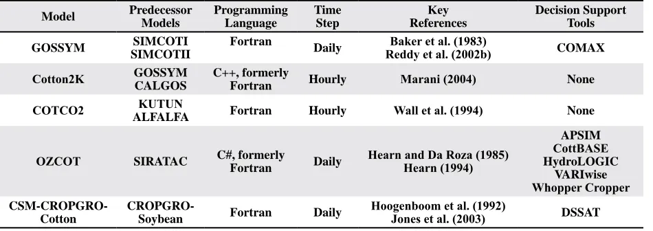
[image:2.612.72.547.572.740.2]cotton plant N balance (Jones et al., 1974), ET, and soil water balance (Ritchie, 1972; Shirazi et al., 1976). Also, the effects of leaf angle and leaf area vertical distribution on light penetration and cotton canopy photosynthesis had been examined using computer models (Fukai and Loomis, 1976). Approaches for simulating the development of cotton fruits, including squares, bolls, seed, and fiber, were investigated later (Jackson et al., 1988; Wanjura and Newton, 1981). Notably, these initial efforts led to the development of the GOSSYM simulation model (Table 1) and the accompany-ing CrOp MAnagement eXpert system (COMAX), which was used across the U.S. Cotton Belt to guide on-farm cotton management in the 1980s (McKinion et al., 1989; Whisler et al., 1986).
Table 1. General information on existing cotton simulation models.
Model Predecessor Models
Programming Language
Time Step
Key
References
Decision Support Tools
GOSSYM SIMCOTI SIMCOTII
Fortran
Daily Reddy et al. (2002b)Baker et al. (1983) COMAX
Cotton2K GOSSYMCALGOS C++, formerly Fortran Hourly Marani (2004) None
COTCO2 ALFALFAKUTUN Fortran Hourly Wall et al. (1994) None
OZCOT SIRATAC C#, formerly
Fortran Daily
Hearn and Da Roza (1985) Hearn (1994)
APSIM
CottBASE
HydroLOGIC VARIwise
Whopper Cropper
CSM-CROPGRO-Cotton
CROPGRO-Soybean Fortran Daily
Hoogenboom et al. (1992)
In addition to GOSSYM/COMAX, other simulation models for cotton production systems were developed more recently (Table 1): Cotton2K (Marani, 2004), COTCO2 (Wall et al., 1994), OZCOT (Hearn, 1994), and CROPGRO-Cotton (Jones et al., 2003; Pathak et al., 2007, 2012). A variety of generic cropping system models, with reduced complexity for simulating a variety of crop types, were also recently evaluated for cot-ton production (Farahani et al., 2009; Sommer et al., 2008; Zhang et al., 2008). The models vary greatly in details and approaches for simulating various plant and soil processes and manage-ment practices, and none have yet reached their full potential. Landivar et al. (2010) provided an excellent review of strategies for physiological simulation of cotton growth and development; however, “it [was] not the purpose of this chapter to compare cotton models.” Landivar et al. (2010) mainly described model development approaches and did not contrast existing cotton models or re-view recent advances in cotton model applications. The objective of this article was to review the state of the art in development and application of computer simulation models for cotton production systems. Be-cause of its comprehensive scope, cotton researchers with diverse interests and levels of expertise should find useful information herein. Given the trend for new cotton modeling efforts beyond traditional analyses of agronomic field experiments, the review also provides a resource for nontraditional and beginning modelers to learn about past and present cotton modeling efforts. A brief history is presented of cotton model develop-ment and applications in the last century, from 1960 to 2000. Descriptions and qualitative comparisons of existing cotton models are emphasized in this section. Next, the review describes cotton model development and applications in the current century thus far. Since year 2000, the literature has demonstrated a marked increase in journal articles that describe applications of the cotton models previously developed, and fewer articles focus on development of new models. Finally, considering the reviewed literature holistically, a per-spective is provided on anticipated future challenges and opportunities for the application of process-based simulation models to cotton production.
PAST DIRECTIONS: 1960-2000
Overview of Simulation Approaches. The cotton models discussed herein are classified as
mechanistic, dynamic, and deterministic. The models are mechanistic as they describe pro-cesses with some level of understanding (e.g., plant growth based on calculations of intercepted radiation). They are dynamic, because the time variable is explicit. Thus, the models use partial differential equations to calculate how quanti-ties vary with time (e.g., transpiration and plant growth). The models are deterministic rather than stochastic, because the calculations are made without any associated probability distribution. Although most cotton simulation models share
these characteristics, different model design strategies have been explored. For example, the cotton model of Plant et al. (1998) used qualita-tive categorical variables (e.g., HIGH, MODER-ATE, or LOW) rather than quantitative variables to describe plant and soil states. The coarseness of the Plant et al. (1998) model improved simula-tion robustness at the expense of precision, but the model was arguably less mechanistic and dynamic than traditional cotton models. Most cotton models simulate soil and plant processes explicitly and quantitatively in a mechanistic, dynamic, and deterministic fashion.
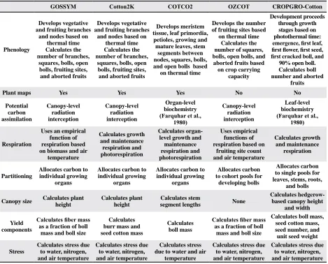
Process-based crop models share a common goal of estimating crop yield by simulating the contribution of soil water, nutrient, and plant growth and developmental processes to the forma-tion of harvestable plant products. However, the approaches used to simulate these processes vary widely among existing crop models (Tables 2 and 3; Landivar et al., 2010). To simulate plant devel-opment, many crop models use a growing degree-day concept, where measured air temperature is assessed in relation to known functions of crop development rate with air temperature. Simulation details, such as the number of development stages considered, the treatment of leaf appearance, and the development of yield components, vary widely among models (Table 2). Carbon (C) assimilation and biomass accumulation are commonly simulated as a function of measured solar irradiance, using simulated leaf area index (LAI) to calculate the fraction of photosynthetically active radiation in-tercepted by the crop canopy. Simulations of water, nutrient, and temperature stresses and atmospheric carbon dioxide (CO2) concentrations ([CO2]) can
Table 2. Crop growth and development processes simulated by existing cotton simulation models.
GOSSYM Cotton2K COTCO2 OZCOT CROPGRO-Cotton
Phenology
Develops vegetative and fruiting branches
and nodes based on thermal time Calculates the number of branches,
squares, bolls, open bolls, fruiting sites, and aborted fruits
Develops vegetative and fruiting branches
and nodes based on thermal time Calculates the number of branches,
squares, bolls, open bolls, fruiting sites, and aborted fruits
Develops meristem tissue, leaf primordia, petioles, growing and mature leaves, stem
segments between nodes, squares, bolls, and open bolls based
on thermal time
Develops the number of fruiting sites based
on thermal time Calculates the number of squares, bolls, open bolls, and
aborted fruits based on crop carrying
capacity
Development proceeds through growth stages based on photothermal time:
emergence, first leaf, first flower, first seed, first cracked boll, and
90% open boll. Calculates boll number and aborted
fruits
Plant maps Yes Yes Yes No No
Potential carbon assimilation Canopy-level radiation interception Canopy-level radiation interception Organ-level biochemistry
(Farquhar et al., 1980) Canopy-level radiation interception Leaf-level biochemistry
(Farquhar et al., 1980)
Respiration
Uses an empirical function of respiration based on biomass and air
temperature Calculates growth and maintenance respiration and photorespiration Calculates organ-level growth and maintenance respiration and photorespiration
Uses empirical functions of respiration based on
fruiting site count and air temperature
Calculates growth and maintenance
respiration
Partitioning
Allocates carbon to individual growing
organs
Allocates carbon to individual growing
organs
Allocates carbon to individual growing
organs
Allocates carbon to cohort pools for
developing bolls
Allocates carbon to single pools for leaves, stems, roots,
and bolls
Canopy size Calculates plant height
Calculates plant height
Calculates stem
segment lengths None
Calculates hedgerow-based canopy height
and width
Yield components
Calculates fiber mass
as a fraction of boll mass and boll size
Calculates burr mass and seed cotton mass
Calculates boll mass
Calculates fiber mass
as a fraction of boll mass and boll size
Calculates boll mass, seed cotton mass, seed number, and unit seed weight
Stress
Calculates stress due to water, nitrogen, and air temperature
Calculates stress due to water, nitrogen, and air temperature
Calculates stress due to water and air
temperature
Calculates stress due to water, nitrogen, and air temperature
Calculates stress due to water, nitrogen, and air temperature
Table 3. Atmospheric and soil processes simulated by existing cotton simulation models.
GOSSYM Cotton2K COTCO2 OZCOT CROPGRO-Cotton
[CO2] effect on
photosynthesis Yes Yes Yes No Yes
[CO2] effect on
transpiration No No Yes No Yes
ET Ritchie (1972)
Modified Penman equation from CA Irrigation Management Information System Leaf-level energy balance coupled with stomatal conductance
Richie (1972) Priestley and Taylor (1972) and FAO-56 (Allen et al., 1998)
Soil water
2D RHIZOS model (Lambert et al.,
1976)
2D RHIZOS model (Lambert et al.,
1976) 2D model Ritchie (1972)
Ritchie (1998) and Ritchie et al. (2009)
Soil nitrogen
Dynamic simulation of soil and plant nitrogen balances
Dynamic simulation of soil and plant nitrogen balances
No
Static, empirical approach that predicts potential N
uptake
Godwin and Singh
(1998) or Gijsman et al. (2002)
Soil phosphorus No No No No Yes
Soil salinity No Yes No No No
Waterlogging No No No Yes Yes
[image:4.612.73.540.490.739.2]Perhaps the most important physiological differ-ence among models is whether they use a radiation use efficiency approach to account for plant growth and maintenance respiration (Monteith, 1977) or whether they explicitly simulate photosynthesis and respira-tion as independent processes (Boote and Pickering, 1994; Farquhar et al., 1980; McCree, 1974; Mutsaers, 1982; Penning de Vries, 1975; Penning de Vries et al., 1974). Models also differ in simulation details for leaf
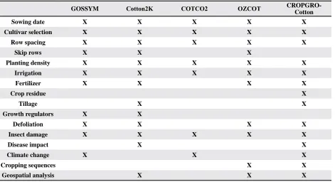
area expansion, stem elongation, organ growth, and yield components. To simulate the soil water balance, several crop models implement the “tipping bucket” method of Ritchie (1972, 1998), whereas others use numerical methods to solve the soil water balance. Simulations of ET are conducted using a variety of methods with varying complexity and data require-ments: Priestley and Taylor (1972); FAO-56 Penman-Monteith (Allen et al., 1998); or surface energy bal-ance. Approaches to simulate N dynamics are also variable, whereas some models do not simulate any nutrient effect on plant growth (Table 3). Models also vary in their consideration of management impacts on cotton production, including irrigation, fertilization, sowing date, tillage, and defoliation events (Table 4). The time steps of calculations also vary among models, but hourly or daily time steps are common (Table 1). Given the diverse approaches for simulating cotton production systems, it is not the objective of this re-view to claim one approach as superior to the other,
but rather to summarize and contrast the approaches currently implemented in existing cotton models. The appropriateness of a given model will depend mainly on the specific application.
Established Crop Simulation Models for Cotton
[image:5.612.74.545.483.739.2]GOSSYM. The development, characteristics, and applications of the cotton model, GOSSYM, were previously described extensively (Baker et al., 1983; Hodges et al., 1998; Landivar et al., 2010; McKin-ion et al., 1989; Reddy et al., 1997a, 2002a). Briefly, GOSSYM uses mass balance principles to simulate water, C, and N processes in the plant and soil root zone. It requires environmental variables, such as solar irradiance, air temperature, precipitation, and wind, as well as information on soil physical properties and cultural practices, including variety-dependent parameters. The model estimates potential growth and developmental rates as a function of air temperature under optimum water and nutrient conditions, and it reduces the potential rates by the intensity of envi-ronmental stresses using envienvi-ronmental productivity indices (Baker et al., 1983; Reddy et al., 2008). Each day, the model simulates the birth and abscission of organs, their size and growth stage, and the intensity of stress factors. The user can assume certain future weather conditions (days, weeks, and years) to de-termine fiber yield estimates and impact of altered cultural practices on cotton maturity and fiber yield.
Table 4. Management practices simulated by existing cotton simulation models and other applications.
GOSSYM Cotton2K COTCO2 OZCOT
CROPGRO-Cotton
Sowing date X X X X X
Cultivar selection X X X X X
Row spacing X X X X X
Skip rows X X X
Planting density X X X X X
Irrigation X X X X X
Fertilizer X X X X
Crop residue X
Tillage X X
Growth regulators X X
Defoliation X X X X
Insect damage X X X X X
Disease impact X X
Climate change X X X
Cropping sequences X X
The GOSSYM model consists of several subrou-tines for various aspects of crop production (Hodges et al., 1998) and biology (Reddy et al., 1997a). A unique aspect is its treatment of the soil (Lambert et al., 1976) and the processes therein, as they influ -ence the plant’s physiological processes. In addition to plant and soil processes, an expertsystem known asCOMAX was explicitly developed for the GOS-SYM model (Hodges et al., 1998; Lemmon, 1986; McKinion et al., 1989).
The concept and development of GOSSYM started in the late 1960s with a meeting at the Uni-versity of Arizona, sponsored by the Department of Agronomy and Agricultural Engineering (Baker et al., 1983; Hodges et al., 1998; Landivar et al., 2010; Reddy et al., 2002b). Significant contributions were made from several institutions (Baker et al., 1972, 1976, 1983; Hesketh and Baker, 1967; Hesketh et
al., 1971, 1972; Lambert et al., 1976; McKinion et al., 1975; Wanjura et al., 1973) in the years after that first meeting.
With the construction of Soil-Plant-Atmosphere-Research facilities at several locations in the south-eastern U.S. (Phene et al., 1978; Reddy et al., 2001), cotton physiological, growth, and developmental processes as affected by abiotic stress factors were quantified. Based on data from these facilities, al -gorithms were developed to improve the model’s functionality and accuracy of simulation results (Ma-rani et al., 1985; Reddy et al., 1993, 1995, 1997a,b, 2000, 2001, 2003). In 1984, GOSSYM was first implemented on commercial cotton farms as a deci-sion support system (DSS). Based on user requests, the COMAX interface was developed to facilitate its delivery to over 70 cotton farms across the U.S. Midsouth. By 1990, GOSSYM-COMAX had been implemented on more than 300 commercial farms (Ladewig and Taylor-Powell, 1989; Ladewig and Thomas, 1992). Extensive model validation efforts were conducted across the U.S. Cotton Belt (Boone et al., 1993; Fye et al., 1984; Reddy, 1994; Reddy and Baker, 1988, 1990; Reddy and Boone, 2002; Reddy et al., 1985, 1995; Staggenborg et al., 1996) and overseas (Gertsis and Symeonakis, 1998; Gertsis and Whisler, 1998). Several modifications in the simulation procedures and model validation efforts using field data sets (Ali et al., 2004; Khorsandi and Whisler, 1996; Khorsandi et al., 1997) made the model applicable on many fronts, including farm management, economics, climate change, and policy issues (Doherty et al., 2003; Landivar et al., 1983a,b;
Liang et al., 2012a,b; McKinion et al., 1989, 2001; Reddy et al., 2002b; Wanjura and McMichael, 1989; Watkins et al., 1998; Xu et al., 2005).
Cotton2K. The Cotton2K model was developed by Dr. Avishalom Marani at the School of Agricul-ture of the Hebrew University of Jerusalem. The source code of Cotton2K is written in C++ and is
available for free download (Marani, 2004). Cot-ton2K uses the process-based equations of GOSSYM (Baker et al., 1972, 1983), and its history can be traced and linked to other cotton modeling efforts, including SIMCOTI (Baker et al., 1972), SIMCOTII (Jones et al., 1974), and CALGOS (Marani et al., 1992a,b,c). The main purpose of Cotton2K was to
provide a more useful model for cotton production in arid, irrigated environments, such as the western U.S. and Israel.
the calculation and the integration of differential equations on an hourly time-step for the processes of plant transpiration, soil water evaporation, soil water redistribution, heat and N fluxes, and the exchanges of energy and water at the soil-plant-atmosphere interfaces. These modifications greatly improved the utility and the applicability of Cotton2K for ir-rigation in arid environments.
The main processes calculated in Cotton2K are related to the exchanges of energy and water between the soil, plant, and the environment. Processes are based on the principles of mass and energy conserva-tion, whereby inputs and outputs to the system are balanced and accounted for as a function of time. The Cotton2K model was designed for specific management of agronomic inputs, including irriga-tion, N fertilizer, defoliairriga-tion, and application of a plant growth regulator. Plant growth and develop-ment are based on the “stress” theory (Craine, 2005; Grime, 1977), which includes stresses related to air temperature, water, C, and N. In this context, stress is a condition that restricts potential production due to suboptimal air temperatures and shortages of water and nutrients (Grime, 1977). Plant growth rates are related to ambient temperature using the concept of heat units (Peng et al., 1989; Wang, 1960). Potential growth rates of all plant organs, including roots, stems, leaf blades and petioles, and fruiting sites (squares, bolls, and seed cotton), are related to source-sink relations of C and water via stress factors. The stress factors between source and sink vary nu-merically from 1 (no stress) to 0 (severe stress). The C stress is related to net C assimilation (i.e., gross photosynthesis minus photorespiration and growth and maintenance respiration). The water stress is related to transpiration and transport of water as a function of leaf water potential. The N stress is based on supply and demand of N. In the soil, Cotton2K calculates rates of available N from urea hydrolysis, mineralization of organic N, nitrification of ammo -nium, denitrification of nitrate, and movement of soluble N. The model also calculates the N in plant organs (roots, stems, leaves, and fruiting sites) and, if supply does not meet requirements, an N stress factor is calculated. All supply and demand functions related to temperature, water, C, and N are dynamic and thus their values change with time.
The boundary conditions that define the one-dimensional soil-plant-atmosphere system in Cot-ton2K are 2 m above and 2 m below the soil surface. The height (2 m) above the soil surface represents
the screen-height where input weather data are mea-sured, and the soil depth of 2 m represents the lower boundary of the soil profile. Required input weather data include shortwave irradiance, air temperature, humidity, wind speed, and rainfall. Cotton2K uses hourly weather input values; however, if not available, daily values of radiation and wind run, and maximum and minimum values of air temperature and humid-ity are used to calculate hourly values (Ephrath et al., 1996). For each irrigation event, the application method (sprinkler, furrow, and drip), timing (start and end), and applied depth are specified. The user defines the geometry of the soil profile by specifying the number and the thickness of each soil layer. At the onset of simulation, (i.e., time = 0), the user speci-fies for each soil layer a value of temperature, water, organic matter, N, and soil salinity. In addition, the soil layers are grouped into horizons, each having unique soil hydraulic properties. These properties define the relationship of soil water content to water potential and to hydraulic conductivity and are used in Richards’ equation to calculate water movement in the soil profile. The user specifies the water table depth and the date and depth of each cultivation event. Other fixed parameter input values are location (latitude, longitude, and elevation), start and end of simulation period, date of planting and/or emergence, and field data (planting density and row spacing, in -cluding skip rows). Parameters describing individual cultivars affect phenology, growth, and development and ultimately impact the calculation of cotton fiber yield as suggested by Marani (2004) and shown by Booker (2013). The current version of Cotton2K has been tested for six cotton cultivars: Acala SJ-2, GC-510, Maxxa, Deltapine 61, Deltapine 77, and Sivon.
The Cotton2K model has been directly and indi-rectly used and tested by many researchers. Diindi-rectly, Cotton2K has been used by Yang et al. (2008) where the effect of pruning and topping was tested under field conditions and by Yang et al. (2010) and Nair et al. (2013) to optimize irrigation allocation under limited water conditions. Recently, Booker (2013) incorporated Cotton2K into a landscape-scale model and applied it to cotton production across the major soil types of the Texas High Plains. Given the similari-ties of Cotton2K to GOSSYM and CALGOS models, indirectly some of the algorithms in Cotton2K have been evaluated for a wide range of soil and envi-ronmental conditions by Staggenborg et al. (1996), Clouse (2006), Baumhardt et al. (2009), and others.
COTCO2. The COTCO2 model simulates cot-ton physiology, growth, development, water use, biomass, and boll yield (Wall et al., 1994). Writ-ten in Fortran in a modular design, it is capable of simulating cotton crop responses to elevated [CO2] and potential concomitant changing climate
variables, particularly temperature. Explicit physi-ological mechanisms are used to minimize reliance on empirical relationships, which are data dependent. The morphogenetic template concept in the KUTUN model (Mutsaers, 1984) and the physiological detail in an alfalfa model, ALFALFA (Denison and Loomis, 1989), served as prototypes for the COTCO2 model.
Leaf physiology is central to simulating plant response to the environment in COTCO2 and con-sists of the following components, which are simu-lated hourly: 1) leaf energy balance to account for stomatal effects on leaf temperature, transpiration, and assimilation; 2) stomatal conductance coupled with leaf energy balance; 3) biochemical chloroplast CO2 assimilation; 4) apparent dark respiration for
each organ type based on basal coefficients for the quantitative biochemistry of biosynthesis of existing phytomass (maintenance respiration) and that linked to growth (growth respiration); and 5) carbohydrate pool dynamics.
Growth is simulated for individual meristem, stem segment, leaf blade, taproot, lateral root, and fruit (squares and bolls) organs. Potential growth is calculated, followed by the carbohydrate and N required to meet potential growth. Actual growth is based on potential growth, substrate availability, and water and temperature stress. Physiological age, which is the time-integrated value of developmen-tal rate, places an upper limit on growth rate, and physiological age determines organ phenological
state. The phenology of the simulated cotton plant does not develop based on calendar days. Rather, plant development and growth rates are based on a time-temperature running sum. The response of physiological time to temperature is based on an Ar-rhenius equation with both low and high temperature inhibition. At the reference temperature (e.g., 25° C), physiological time is equal to calendar days. Within the low and high temperature limits, physiological time proceeds faster and slower than calendar time at temperatures higher and lower than the reference temperature, respectively.
The COTCO2 model can simulate cotton pro-duction over a broad environmental range, while providing the means to predict the impact of change in [CO2] and any associated potential climate change
on global cotton production. Ultimately, it could aid in the development of strategies to mitigate the adverse effects of global climate change, while optimizing those that are beneficial.
OZCOT. The structure of the OZCOT model has been described in detail by Hearn (1994) and Hearn and Da Roza (1985). It was developed using a top-down approach, meaning processes were simulated with only sufficient detail to provide reliable estima -tion of the impact of management and environment on cotton growth, development, and fiber yield. Simulation approaches were broadly mechanistic at the crop and plant level. The OZCOT model, which advances on a daily time step, is principally driven by air temperature and intercepted radiation, and it was built by linking a model of fruiting dynamics with a water balance model and simple N uptake model. In addition to validation using research experiments (Hearn, 1994), OZCOT also has been validated in commercial fields for both irrigated (Richards et al., 2008) and rainfed cotton systems (Bange et al., 2005).
Carbon supply for a given day is estimated from intercepted light and a canopy-level photosynthetic rate (Baker et al., 1983), with respiration calculated as an empirical function of fruiting site count and mean air temperature. Light interception is estimated using Beer’s law, and leaf area is simulated using an empirical correlation between fruiting site production and leaf area (Jackson et al., 1988). The rates of leaf expansion, photosynthesis, and fruiting are modulated by the supply of water and N and by waterlogging.
The water balance in OZCOT is calculated using the Ritchie (1972) approach with a calibrated soil water extraction routine based on increasing supply with increasing depth of extraction over time. The OZCOT model does not maintain a dynamic soil N balance analogous to water, but uses an N uptake model. At the start of the season, potential N uptake is estimated based on soil N and fertilizer inputs (Constable and Rochester, 1988) and is reviewed daily to calculate a stress index. The stress index scales the rate of a process and is based on the ratio either between supply and demand for a resource or between the current and maximum value of a state variable. In addition to N, there are also stress indices for shortages of water and C.
The OZCOT model can be principally used in two modes: a strategic mode that generates simula-tions over multiple seasons using pre-determined management rules and historical climate data or a tactical mode that simulates specific management practices for a particular season. In both modes, daily values of rainfall (mm), maximum and minimum air temperature (degrees C), and solar irradiation (MJ m-2) are required. Relative humidity at 0900 h and
wind run (km) can also be included for improved pre-cision of daily ET estimates. Soil input information includes the number of soil layers and their depths, plant available water holding capacity, initial plant available water (in volumetric units), and average soil bulk density across layers.
Agronomic inputs include parameters for dif-ferent cotton cultivars, including leaf type (okra or palmate), squaring rate, maximum boll size and development rate, fiber percentage, background fruit retention (transgenic or non-transgenic), row spac-ing, plants per meter of row, initial available soil N, irrigation rates and application dates, N rates and application dates, and planting dates. If a specific planting date or days when irrigation occurs is not provided, management rules are used to estimate these times in the strategic mode.
The OZCOT model can simulate production in rainfed or limited irrigation cropping systems using “skip row” configurations (Bange et al., 2005). These are row configurations that have entire rows missing from the planting configuration to increase the amount of soil water available to the crop at critical growth stages. The OZCOT model uses a modified soil water content stress index that accounts for the non-uniform distribution of the availability of soil water from the planted and non-planted rows (Milroy et al., 2004).
Key outputs generated by the OZCOT model include seasonal estimates of fiber yield, yield com -ponents, dates of phenological stages, maximum LAI, N use, and water balance metrics such as effective rainfall and crop water use efficiency (WUE). A separate output file is also generated that provides daily within-season calculations of crop progress, stress indices, and resource use.
The OZCOT model is the only supported cotton model in Australia that is used in decision support and research. Currently, the OZCOT model is the core component of the HydroLOGIC tactical and strategic cotton irrigation DSS (Richards et al., 2008). To refine simulations of in-season crop water use in HydroLOGIC, OZCOT was modified to accept ad -ditional measurements of soil water status and crop growth, such as LAI and fruit number. Other DSSs that have used OZCOT include CottBASE (https:// cottassist.com.au) for irrigated cotton systems and Whopper Cropper (Nelson et al., 2002) for rainfed cotton systems. Both are databases of pre-run OZ-COT simulations based on historical climate data for various combinations of management options, soils, and regions.
Until recently, OZCOT was written in Fortran and compiled as a dynamic link library. Currently called “mvOZCOT”, the OZCOT model has been rewritten in C# and was reengineered using the common modeling protocol of the Commonwealth Scientific and Industrial Research Organisation (CSIRO) to allow more seamless integration with APSIM and other modeling frameworks (Moore et al., 2007). This has enabled OZCOT users to imple-ment the model with other soil water and N modules. Although OZCOT continues to be used as a research
and management tool, current efforts to enhance its functionality include the addition of new algorithms to simulate fiber quality and climate change impacts.
CSM-CROPGRO-Cotton. The Cropping System Model (CSM)-CROPGRO-Cotton model (Jones et al., 2003; Pathak et al., 2007) is implemented in the Decision Support System for Agrotechnology Transfer (DSSAT; Hoogenboom et al., 2012). The DSSAT system has a long history originating with the International Benchmark Sites Network for Agrotechnology Transfer (IBSNAT) Project that was funded by the U.S. Agency for International Development from 1982 through 1993 (Uehara and Tsuji, 1989). The initial crop simulation models of DSSAT included the Wheat, CERES-Maize, SOYGRO, and PNUTGRO models. The SOYGRO, PNUTGRO, and BEANGRO models were later combined into a generic grain legume model, CROPGRO (Hoogenboom et al., 1992). To address cropping systems and especially crop rota-tions, the CSM was developed (Jones et al., 2003). The CSM model uses a single set of computer code for dynamic simulation of the soil water, inorganic soil N, and organic C and N balances (Gijsman et al., 2002; Godwin and Singh, 1998; Ritchie, 1998, Ritchie et al., 2009). Recently a soil phosphorus module also was added to CSM (Dzotsi et al., 2010). For the simulation of growth, development, and ultimately yield for individual crops, different crop modules are being used, such as the CERES-Maize module for maize (Zea mays L.), CERES-Rice for rice (Oryza sativa L.; Ritchie et al., 1998) or the CROPGRO module for grain legumes (Boote et al., 1998). This allows for the continuous simulation of crop rotations, such as a soybean (Glycine max (L.) Merr.) and wheat (Triticum aestivum L.) rotation or a wheat and rice rotation (Bowen et al., 1998; Tojo Soler et al., 2011).
The CROPGRO module uses a daily time step for integration, starting at planting and ending at crop
maturity or on the user-specified harvest date. The differences among the individual crops or species are handled through external genotype files, as opposed to values or specific equations that are embedded in the code. There are three genotype files: one each for cultivar, ecotype, and species coefficients (Hoogenboom and White, 2003). The latter includes a range of temperature functions for development, photosynthesis, partitioning, and various other physi-ological functions. It also includes detailed composi-tion parameters with respect to proteins, lipids, fiber, carbohydrates, and other properties of different plant components, including leaves, stems, roots, and reproductive structures. This approach assumes that the underlying plant physiological processes of each crop are similar, but the interaction of genetics with environment and management is different.
The original DSSAT systems did not include a model for fiber crops. Because of the importance of cotton in the southeastern U.S., especially as part of common rotations with peanut (Arachis hypogaea
L.), there was a need for the development of a com-prehensive cotton model. Rather than developing a new set of code, the decision was made to use the CROPGRO module as a template. The emphasis was to obtain detailed physiological information to define the functions and parameters for the species file and experimental data for initial model calibra -tion and evalua-tion. The CSM-CROPGRO-Cotton model was developed through a collaborative effort among scientists at the University of Florida and the University of Georgia (Pathak et al., 2007). Because of the existing infrastructure of DSSAT, the cotton model could easily be added to DSSAT without creat-ing different utilities for data input and application programs.
file, which is based on the CO2 values measured at
the long-term CO2 monitoring site on Mauna Loa in
Hawaii. Crop management practices include planting date; plant density and row spacing; planting depth; dates and amounts of irrigation application; dates, amounts, and type of fertilizer application; and dates, types, and depths of tillage. Environmental modifica -tions, including climate change modifica-tions, can be entered in the environmental modification section of the crop management file.
As stated previously, the genetic information is provided in three data files. The species file is as -sociated with a specific crop and is part of the core model development and calibration. Therefore, end users should not modify parameters in the species file. The cultivar parameter file specifies 18 cultivar-specific parameters for each cultivar. These include coefficients that describe the time from emergence to flowering, time from flowering to first boll and first seed, time from first seed to physiological maturity, maximum single leaf photosynthetic rate, single leaf size, specific leaf area, individual seed size, fraction of seed cotton weight over total green boll weight, and oil and protein composition of the seeds. The cultivar file that is distributed with DSSAT includes a few cultivars for which the cultivar parameters already have been defined, including those for the example experimental files that are distributed with DSSAT. In general, however, users must calibrate their cultivar parameters using a set of measured data from either experiments or variety trials (Pathak et al., 2012). The ecotype file includes 17 parameters that define the unique characteristics of a group of cultivars, such as a short-season versus a long-season cultivar, and they normally will not change among a group of similar cultivars.
In CSM-CROPGRO-Cotton, the overall inte-gration of differential equations occurs on a daily time step. The CSM is written in Fortran (Thorp et al., 2012), and the software code includes different sections for model initialization, calculation of the rate variables, integration of the equations, and up-date of the state variables. Both daily and seasonal output routines are available (Jones et al., 2003). The model is initiated at the start of simulation, which can occur at or prior to planting. At this point, the initial or boundary conditions are set, especially with respect to initial soil water content, inorganic soil N, soil organic C, and residue remaining from the previous crop. If the model is started prior to planting, only the soil processes are simulated. When
planting occurs, the crop growth module is initiated and vegetative development is simulated. Internally, both the vegetative and reproductive development processes are calculated on an hourly basis, whereas integration occurs at a daily level. Hourly ambient temperature is calculated internally based on the maximum and minimum daily air temperature. In parallel to crop development, photosynthesis is simu-lated on an hourly basis based on light interception of a hedgerow canopy, and integration occurs on a daily basis (Boote and Pickering, 1994). The model accounts for maintenance respiration based on cur-rent total biomass, for growth respiration based on partitioning to the different plant organs, including roots, stems, leaves, bolls, and seed cotton, and for the composition of each organ.
During vegetative growth, partitioning to roots, leaves, and stems is a function of the development stage and is source-driven. However, once reproduc-tive development has started, partitioning is sink-driven based on the requirements for carbohydrates for the reproductive structures, including the bolls. Any remaining carbohydrates that are not used for
growth of the reproductive structures can be used for further growth of the vegetative structures. Once flowering has started, the model accounts for the number of flowers that are formed on a given day, called clusters. This system is maintained through the entire reproductive process, allowing for the abortion of flowers, squares, and bolls if insufficient carbo -hydrates are available for reproductive growth. The priority of the carbohydrate distribution is based on the status of the cohorts; the ones that were formed first have the highest priority for carbohydrates and the ones that were formed last have the lowest prior-ity. During reproductive growth, remobilization of N from senesced leaves and petioles can also occur to support reproductive growth. Most of the growth, development, and partitioning processes have their own temperature response functions that are defined in the species file.
irradiance and maximum and minimum air tem-peratures as input (Priestley and Taylor, 1972). An option is also available to use the Penman-Monteith equation for calculating potential ET. The soil water balance is based on the tipping bucket approach for a one-dimensional soil profile (Ritchie, 1972, 1998). Each soil horizon or computational soil layer is characterized by the LL, DUL, and SAT, which can be calculated based on soil texture and bulk density using utilities provided with DSSAT. The daily potential ET demand is calculated first, and the potential water supply for root uptake is based on the soil water content of each layer, root distribution, and a root resistance factor. If the potential supply is greater than the potential demand, the supply is set equal to the demand, and the associated processes are updated. If the demand is greater than the supply, transpiration and soil water evaporation are reduced to the simulated supply, and drought stress factors are calculated based on the difference between potential demand and potential supply.
The CSM-CROPGRO-Cotton model includes a detailed soil and plant N balance. Although the original CROPGRO model included N fixation, the modular structure of CSM allows for individual modules to be turned on or off (Jones et al., 2003). A detailed description of the soil N balance is given
by Godwin and Singh (1998), which is the same for all crop modules of the CSM. Soil N includes a myriad of processes that are calculated for each soil horizon or computational layer for the transforma-tion of organic N to inorganic N in the form of nitrate and ammonium. For the calculation of the processes associated with soil organic C and N, there are two options. One is the original model developed by Godwin and Singh (1998), and the other is an ad-vanced approach based on CENTURY (Gijsman et al., 2002). The latter approach is especially suitable for low-input systems or for determining the soil C balance associated with soil C sequestration.
Because of the generic structure of the CROP-GRO model, the CROPCROP-GRO-Cotton module benefits from other model features that were previously added to CROPGRO. One such feature is the generic coupling points that emulate the potential impact of pests and diseases on crop growth and development (Boote et al., 1983, 2008, 2010). These coupling points allow for the removal of tissue of the various organs, a modification of leaf area, a reduction in the availability of carbohydrates, and various others that are specified in a crop-specific pest input file. The
actual removal or changes are provided through a time-series input file. Ortiz et al. (2009) used this option to study the impact of southern root-knot nematodes on biomass growth and seed cotton yield.
Most of the applications of the CSM-CROP-GRO-Cotton model have been conducted in the southeastern U.S., including the determination of irrigation water use in Georgia (Guerra et al., 2007), the impact of climate variability and El Niño/La Niña Southern Oscillation (ENSO) on seed cotton yield under different cotton management options (Garcia y Garcia et al., 2010; Paz et al., 2012), sensitivity to solar irradiance (Garcia y Garcia et al.; 2008) and other inputs (Pathak et al., 2007), and crop insur-ance (Cabrera et al., 2006). Applications beyond the U.S. have been limited, except for a climate change application in Cameroon (Gérardeaux et al., 2013) and a study of irrigation strategies in Australia (Cam-marano et al., 2012).
The CSM-CROPGRO-Cotton model is included in DSSAT (Hoogenboom et al., 2012). The most recent version of DSSAT can be requested from the DSSAT Foundation web site (www.DSSAT.net) at no cost. Utility programs are available within DSSAT for entering experimental and environmental data, as well as measured data, for model calibration and evaluation. DSSAT also includes special application programs for crop sequence or rotation analyses and for seasonal analyses that include economic com-ponents. The source code for the model is available upon request.
Generic crop models. Several generic crop models, which simplify crop growth routines for applicability to a variety of crops, have also been developed, and limited reports are available for the use of such models in cotton. The Environ-mental Policy Integrated Climate (EPIC) model, originally called the Erosion-Productivity Impact Calculator (Williams et al., 1984), simulates the impact of climate and management on soil erosion, water quality, and crop production. The generic crop model in EPIC (Williams et al., 1989) is currently parameterized for approximately 80 crops. Evaluations of the EPIC model have been conducted for cotton systems in Georgia (Guerra et al., 2004) and Texas (Ko et al., 2009a). The Simple and Universal CROp growth Simulator (SUCROS; Van Ittersum et al., 2003) models daily canopy CO2 assimilation for potential production
modi-fied SUCROS (SUCROS-Cotton) to simulate “cut-out”, fruit dynamics, fruit abscission, single boll weight, and fiber yield for cotton. The model was evaluated for a cotton system in China. Another Wageningen crop model, WOrld FOod STudies (WOFOST; Van Diepen et al., 1989; Van Itter-sum et al., 2003), is used for generic crop growth simulations in the Soil-Water-Atmosphere-Plant model (SWAP; Kroes et al., 2008), which simu-lates vadose zone transport of water and solutes. Crop yield in SWAP can also be computed using a simplified crop growth algorithm (Doorenbos and Kassam, 1979). The GRAMI model (Maas, 1993a,b,c) was originally developed to estimate growth and yield of gramineous crops such as wheat, maize, and sorghum (Sorghum bicolor (L.) Moench). The model was specifically designed to accept remote sensing data inputs for improving the accuracy of its crop growth simulation. Ko et al. (2005) modified the original GRAMI model to simulate growth and fiber yield of non-stressed cotton. The Root Zone Water Quality Model (RZ-WQM; Ma et al., 2012) originally incorporated a generic crop growth model but now includes the CSM crop modules (Jones et al., 2003), spe-cifically the CROPGRO-Cotton model for cotton systems. CropSyst (Stöckle et al., 2003) is a daily time-step cropping system model that simulates water and N balances, crop growth and develop-ment, residue recycling, erosion by water, and salinity in response to climate, soils, and manage-ment. Sommer et al. (2008) evaluated CropSyst for cotton in Uzbekistan.
Historic Applications of Cotton Models
In the previous century, cotton simulation models were used to assess irrigation and N fertil-izer management strategies and to understand the effects of climate variability on cotton fiber yield. Many of these early efforts were based on the GOS-SYM model (McKinion et al., 1989). Comparisons of GOSSYM-simulated crop water use with field measurements were an important step to evaluate the model for irrigation management purposes (Asare et al., 1992; Staggenborg et al., 1996). The Australian model, OZCOT, was used to make ir-rigation management decisions in relation to water supply (Dudley and Hearn, 1993a; Hearn, 1992). To characterize N impacts on cotton production, GOS-SYM was used to manage N fertilization events for a field study in South Carolina (Hunt et al., 1998),
to evaluate N fertilizer recovery and residual soil N for cotton systems in Mississippi (Stevens et al., 1996), and to assess the effect of N fertilization rate
and timing on cotton fiber yield over a long-term weather record in West Texas (Wanjura and McMi-chael, 1989). Ramanarayanan et al. (1998) used the EPIC model to optimize N fertilization management in Oklahoma, while considering N recovery in cotton fiber yield and N loss to the environment.
Using GOSSYM, Landivar et al. (1983a) ex-amined effects of the “okra-leaf” trait on cotton fruit abscission and fiber yield. Under favorable N conditions, it appeared that a slight yield advantage with the okra-leaf trait was the result of improved light interception. However, under less favorable conditions, okra-leaf restricted LAI, which reduced yields. In a second paper (Landivar et al., 1983b), photosynthetic rate, specific leaf weight and leaf longevity were varied. Greater photosynthetic rate increased fiber yield, but if increased photosynthesis was achieved through greater specific leaf weight (thicker leaves), no yield benefit occurred. Extending leaf longevity appeared more promising for increas-ing yield, but the model did not deal with possible tradeoffs between leaf longevity and processes such as N remobilization.
Due to concerns of declining cotton fiber yield over several decades, GOSSYM was used to exam-ine climate effects on cotton fiber yield at several locations across the U.S. Cotton Belt (Reddy and Baker, 1990; Reddy et al., 1990; Wanjura and Barker, 1988). Weather variables were shown not to be a driver of fiber yield declines, but increasing ozone level might have reduced fiber yields in Phoenix, AZ and Fresno, CA (Reddy et al., 1989). Small increases (10%) in fiber yield due to elevated CO2 were found
within-season estimates of actual crop growth, such as LAI or ground cover, were obtained from remote sensing data. The model parameters and initial conditions were then iteratively adjusted to minimize the dif-ference between simulated crop growth and the measured growth from remote sensing data (Maas, 1993a,b,c). Finally, Larson and Mapp (1997) used
the COTTAM model (Jackson et al., 1988) to esti-mate cotton production responses and net revenue to various management inputs. The simulation results were then used to evaluate the performance of cot-ton cultivars and to assess planting, irrigation, and harvest decisions under risk. These studies laid the foundation for cotton modeling applications in the new century.
PRESENT DIRECTIONS: 2000-2013
Recent Development of Cotton Models. Studies on the application of cotton simulation models after year 2000 vastly outnumbered the studies reporting new model developments. However, there are a few recent and notable accomplishments in the develop-ment of simulation models for cotton. The AquaC-rop model, supported by the Food and Agriculture Organization (FAO) of the United Nations, is a new generic crop model for simulating yield response to water management (Raes et al., 2009; Steduto et al., 2009). This effort resulted in a simulation model, based on plant physiology and soil water balance, that replaced previous FAO publications for estimat-ing crop productivity in relation to water supply. In a short time, the model has been used for a number of irrigation management studies in cotton, discussed in the next section, and in other crops. Pachepsky et al. (2009) developed and parameterized the new WALL model for cotton, which simulates individual leaf transpiration with emphasis on water movement within the leaf. Finally, Liang et al. (2012a) developed a GOSSYM-based, geographically distributed cotton growth model that has been coupled with the Climate-Weather Research Forecasting Model (Skamarock et al., 2005) for studying the effects of changing climate on cotton production.
The literature demonstrates a significant research thrust toward cotton simulation model development in China, the world’s leading cotton producer. Ma et al. (2005) conducted field studies at four locations in China and developed a simula-tion model for cotton development and fruit forma-tion. Zhu et al. (2007) designed a web-based DSS
for crop management that included process-based simulation models for four crops, including cotton. Li et al. (2009) developed a model for simulating boll maturation, seed growth, and oil and protein content of cottonseed. The model was calibrated and evaluated using experimental data sets from two locations in China. Zhao et al. (2012) focused on cotton fiber production and developed a model for simulating cotton fiber length and strength based on air temperature, solar irradiance, and N effects. Another noteworthy direction of research is the recent development of higher-dimensional models that simulate cotton canopy and root architecture. Coelho et al. (2003) used principles from GOSSYM and DSSAT-CSM to develop a model for simulation of horizontal and vertical distributions of cotton root growth at the field scale. Similarly, simulation of three-dimensional cotton root growth was investigated by Zhang and Li (2006) in China. Hanan and Hearn (2003) linked a model of cotton plant morphogenesis and architecture with OZCOT. The combined models allocated flower buds to assigned positions on the plant, and water, N, and C stresses controlled fruit growth and abortion. Jallas et al. (2009) combined a mechanistic model of crop growth and devel-opment with a three-dimensional model of plant architecture. Together, the two models produced an animated visualization of cotton growth for one or several cotton plants. Alarcon and Sassenrath (2011) analyzed digital images of cotton cano-pies and developed a dynamic model to simulate changes in cotton leaf number and leaf size dur-ing the growdur-ing season. These studies evidence a move toward simulation models that consider the influence of plant architecture on cotton growth, a characteristic that is not considered in most exist-ing cotton models.
Recent Applications of Cotton Models
Crop Water Use and Irrigation Management
Baumhardt et al. (2009) simulated fiber yield using GOSSYM for a 40-yr period at Amarillo, TX and used these data to analyze the impact of irrigation depth, irrigation duration, and initial soil water content on WUE and fiber yield of cotton. At lower initial moisture content, fiber yield and WUE increased with increasing irrigation depth, whereas at higher initial soil water content, WUE was lower for the higher irrigation depth although fiber yield was higher. They also reported that, with low irriga-tion water availability, concentrating the irrigairriga-tion water to a subset of the field area could increase cotton fiber yield.
The CSM-CROPGRO-Cotton model was evalu-ated for simulating cotton growth and development under different irrigation regimes in Georgia and was found to be a promising tool for irrigation scheduling (Suleiman et al., 2007). Simulations of ET were compared with field experimental data from Griffin, GA to evaluate the FAO-56 crop coefficient procedure for irrigation management in deficit irri -gated cotton production. Root mean squared errors between measured and simulated ET ranged from 2.5 to 3.5 mm d-1, and model efficiency statistics
were less than 0.28. These results indicate potential for further refinement of the model’s ET simulation. Guerra et al. (2004) evaluated the EPIC model to simulate cotton fiber yield and irrigation demand in Georgia. The model simulated cotton fiber yield and irrigation requirements with root mean squared deviations of 0.29 t ha-1 and 75 mm, respectively.
The model performance for cotton was better than for soybean and peanut. The EPIC model was also used to compare simulated crop water requirements for cotton, peanut, and corn with the actual irrigation amounts applied by farmers in Georgia (Guerra et al., 2005). This study revealed that EPIC was useful for assessing on-farm irrigation water demand. Guerra et al. (2007) used the CSM-CROPGRO-Cotton model to simulate irrigation applications for individual fields and then used kriging to estimate the spatial distribution of the irrigation water use for cotton in Georgia. The technique enabled estimation of water use at spatial scales more suitable to inform policy makers.
Nair et al. (2013) evaluated Cotton2K for the Texas High Plains by simulating cotton fiber yield for a 110-yr period at Plainview, TX. Sixty-eight differ-ent irrigation treatmdiffer-ents were simulated to analyze the production and profitability impacts of partition -ing a center-pivot irrigated cotton field into irrigated
and dryland areas. By irrigating only a subset of the field area, cotton fiber yield and profitability were increased. The benefit was higher when available irrigation water was low and in low rainfall years.
Ko et al. (2006) used a modified version of GRAMI, capable of within-season calibration us-ing remotely sensed crop reflectance data, to model water-stressed cotton growth at Lubbock, TX. Even though the model adequately simulated cotton growth under deficit irrigation, its performance was unsatisfactory at higher irrigation regimes. Ko et al. (2009b) used data from field trials conducted in Uvalde, TX to calibrate the radiation use efficiency and the light interception coefficient of the EPIC crop model. The calibrated model simulated field conditions with more accuracy and hence could be a better tool to manage irrigation water resources.
Evett and Tolk (2009) reviewed nine papers that used cropping system simulation models to simulate yield and WUE of four crops, including cotton. All the models in these studies simulated WUE with considerable accuracy under well-watered condi-tions, but performed poorly under water stress. Crop growth models are important components of web-based DSSs, which can be used by crop managers for irrigation scheduling decisions (Fernandez and Trolinger, 2007).
Australian cotton production. The Australian cotton model, OZCOT (Hearn, 1994), is commonly used for irrigation water management research and decision support in Australia. It was used extensively to assess potential and risk of productivity and value of improvements in WUE across all Australian cot-ton production regions at the field scale (e.g., Hearn, 1992). The need for these assessments was associated
scheduling (Hearn and Bange, 2002; Richards et al., 2008). Irrigation timing was assessed by varying target soil water deficits for triggering irrigations and then by simple user optimization of fiber yield and water use estimates generated by OZCOT outputs. Simulations of fiber yield and water use were based on potential growth determined by OZCOT and historical climate records for the remainder of the season. HydroLOGIC can also be used in a strategic mode that enables users to explore the fiber yield and water productivity of irrigation management prac-tices (pre- and post-season) under different weather patterns using long-term climate data. In this mode, schedules are user-defined and can irrigate the crop when the soil-water deficit reaches a set level, where the first and final irrigation dates are determined by square and boll development.
Recent advances in irrigation management have included the development of a framework “VARI-wise” that develops and simulates site-specific ir -rigation control strategies (McCarthy et al., 2010). VARIwise divides fields into spatial subunits based
on databases for weather, soil, and plant parameters to better account for field variability. The OZCOT model is used in two capacities in VARIwise: 1) to simulate the performance of the control strate-gies and 2) to calculate the irrigation application that achieves a desired performance objective (e.g., maximized bale yield or water productivity). In the first option, industry standard irrigation management strategies are tested, which apply irrigation to fill the soil profile. In the second option, VARIwise executes the calibrated crop model with different irrigation volumes over a finite horizon (e.g., 5 d) to determine which irrigation volumes and timing achieves the desired performance objective (e.g., maximize bale yield or water productivity) as calculated by the model. The optimal combination is implemented and this procedure is repeated daily to determine the tim-ing of the next irrigation event and the site-specific irrigation volumes. An automatic model calibration procedure for soil water, vegetation, and fruit load was developed to minimize the error between the measured and simulated soil and plant responses (McCarthy et al., 2011). A genetic algorithm was used to refine the soil and plant parameters that characterized cotton development.
Evaluation of VARIwise has shown improve-ments in irrigation WUE for center-pivot irrigated cotton (McCarthy et al., 2010) and surface irriga-tion. The field implementation of VARIwise for
surface irrigation includes irrigation hydraulics to determine the control actions (inflow rate and cut-off time) required to achieve the appropriate irrigation distribution along the furrow as determined by the control strategies. This further improves irrigation efficiencies. McCarthy et al. (2013) reviewed the use of crop models for advanced process control of irrigation and argued that process-based simulation models perform better than crop production func-tions. Significant opportunity remains to further en -hance the VARIwise system by linking the predictive functionalities of HydroLOGIC, which is focused on crop growth performance, with the improved irrigation practice recommendations generated by VARIwise.
On-farm water storage and distribution are limiting factors of the irrigation decision making process for cotton production. The APSIM frame-work incorporates water storage and has enabled the exploration of irrigation management options that rely on effluent water or opportunistic capture of overland flow as water sources (Carberry et al., 2002a). To provide probabilistic forecasts of on-allocation and off-allocation water, catchment models and seasonal climate forecasts have been implemented, and the simulated water supply was used with a cotton simulation model to determine seasonal water requirements and cotton bale yield (Power et al., 2011a,b). The gross margins, water requirements, and subsequent bale yields were then used to evaluate different cropping areas with dif-ferent water availability and management paradigms. Alternatively, the irrigation events were scheduled when the OZCOT-simulated soil water deficit reached a set limit or when OZCOT maximized bale yield (Ritchie et al., 2004). Then, a gross margin model was developed using the seasonal climate forecasts, estimated bale yield, and water application for the given water supply. The resulting bale yield, water and crop production costs, and crop price were provided for each year of the simulation.