Directly comparing GW150914 with numerical solutions of Einstein's equations for binary black hole coalescence

Einstein's equations for binary black hole coalescence

.

White Rose Research Online URL for this paper:

http://eprints.whiterose.ac.uk/107668/

Version: Accepted Version

Article:

Abbott, BP, Abbott, R, Abbott, TD et al. (975 more authors) (2016) Directly comparing

GW150914 with numerical solutions of Einstein's equations for binary black hole

coalescence. Physical Review D, 94 (6). 064035. ISSN 2470-0010

https://doi.org/10.1103/PhysRevD.94.064035

[email protected] https://eprints.whiterose.ac.uk/ Reuse

Unless indicated otherwise, fulltext items are protected by copyright with all rights reserved. The copyright exception in section 29 of the Copyright, Designs and Patents Act 1988 allows the making of a single copy solely for the purpose of non-commercial research or private study within the limits of fair dealing. The publisher or other rights-holder may allow further reproduction and re-use of this version - refer to the White Rose Research Online record for this item. Where records identify the publisher as the copyright holder, users can verify any specific terms of use on the publisher’s website.

Takedown

If you consider content in White Rose Research Online to be in breach of UK law, please notify us by

Directly comparing GW150914 with numerical solutions of Einstein’s equations for binary black

hole coalescence

B. P. Abbott et al.∗

We compare GW150914 directly to simulations of coalescing binary black holes in full general relativity, in-cluding several performed specifically to reproduce this event. Our calculations go beyond existing semianalytic models, because for all simulations – including sources with two independent, precessing spins – we perform comparisons which account for all the spin-weighted quadrupolar modes, and separately which account for all the quadrupolar and octopolar modes. Consistent with the posterior distributions reported in LVC-PE[1] (at the 90% credible level), we find the data are compatible with a wide range of nonprecessingand precessing

simulations. Followup simulations performed using previously-estimated binary parameters most resemble the data, even when all quadrupolar and octopolar modes are included. Comparisons including only the quadrupo-lar modes constrain the total redshifted massMz ∈ [64M⊙−82M⊙], mass ratio 1/q=m2/m1 ∈ [0.6,1], and effective aligned spin χeff ∈ [−0.3,0.2], whereχeff = (S1/m1+S2/m2)·Lˆ/M. Including both quadrupolar and octopolar modes, we find the mass ratio is even more tightly constrained. Even accounting for precession, simulations with extreme mass ratios and effective spins are highly inconsistent with the data, at any mass. Several nonprecessing and precessing simulations with similar mass ratio andχeff are consistent with the data. Though correlated, the components’ spins (both in magnitude and directions) are not significantly constrained by the data: the data is consistent with simulations with component spin magnitudesa1,2up to at least 0.8, with random orientations. Further detailed followup calculations are needed to determine if the data contain a weak imprint from transverse (precessing) spins. For nonprecessing binaries, interpolating between simulations, we reconstruct a posterior distribution consistent with previous results. The final black hole’s redshifted mass is consistent withMf,zin the range 64.0M⊙−73.5M⊙and the final black hole’s dimensionless spin parameter is

consistent withaf =0.62−0.73. As our approach invokes no intermediate approximations to general relativity and can strongly reject binaries whose radiation is inconsistent with the data, our analysis provides a valuable complement to LVC-PE[1].

I. INTRODUCTION

On September 14, 2015 09:50:45 UTC, gravitational waves were observed in coincidence by the twin instruments of the Laser Interferometer Gravitational-wave Observatory (LIGO) located at Hanford, Washington, and Livingston, Louisiana, in the USA, an event known as GW150914[2]. LVC-detect[2], LVC-PE[1], LVC-TestGR[3], and LVC-Burst[4] demonstrate consistency between GW150914 and selected individual pre-dictions for a binary black hole coalescence, derived using numerical solutions of Einstein’s equations for general rela-tivity. LVC-PE[1] described a systematic, Bayesian method to reconstruct the properties of the coalescing binary, by com-paring the data with the expected gravitational wave signa-ture from binary black hole coalescence [5], evaluated using state-of-the-art semianalytic approximations to its dynamics and radiation [6–8].

In this paper, we present an alternative method of recon-structing the binary parameters of GW150914, without using the semianalytic waveform models employed in LVC-PE[1]. Instead, we compare the data directly with the most physi-cally complete and generic predictions of general relativity: computer simulations of binary black hole coalescence in full nonlinear general relativity (henceforth referred to as numeri-cal relativity, or NR). Although the semianalytic models are calibrated to NR simulations, even the best available

mod-∗_{Full author list given at the end of the article}

els only imperfectly reproduce the predictions of numerical relativity, on a mode-by-mode basis [9]. Furthermore, typi-cal implementations of these models, such as those used in LVC-PE[1], consider only the dominant spherical-harmonic mode of the waveform (in a corotating frame). For all NR simulations considered here—including sources with two in-dependent, precessing spins—we perform comparisons that account for all the quadrupolar spherical-harmonic waveform modes, and separately comparisons that account for all the quadrupolar and octopolar spherical harmonic modes.

The principal approach introduced in this paper is different from LVC-PE[1], which inferred the properties of GW150914 by adopting analytic waveform models. Qualitatively speak-ing, these models interpolate theoutgoing gravitational wave strain(waveforms) between the well-characterized results of numerical relativity, as provided by a sparse grid of simula-tions. These interpolated or analytic waveforms are used to generate a continuous posterior distribution over the binary’s parameters. By contrast, in this study, we compare numerical relativity to the data first, evaluating a single scalar quantity (the marginalized likelihood) on the grid of binary parame-ters prescribed and provided by all available NR simulations. We then construct an approximation to the marginalized like-lihood that interpolates between NR simulations with different parameters. To the extent that the likelihood is a simpler func-tion of parameters than the waveforms, this method may re-quire fewer NR simulations and fewer modeling assumptions. Moreover, the interpolant for the likelihood needs to be accu-rate only near its peak value, and not everywhere in parameter space. A similar study was conducted on GW150914 using a

subset of numerical relativity waveforms directly against re-constructed waveforms [4]; the results reported here are con-sistent but more thorough.

Despite using an analysis that has few features or code in common with the methods employed in LVC-PE[1], we arrive at similar conclusions regarding the parameters of the progen-itor black holes and the final remnant, although we extract slightly more information about the binary mass ratio by using higher-order modes. Thus, we provide independent corrobo-ration of the results of LVC-PE[1], strengthening our confi-dence in both the employed statistical methods and waveform models.

This paper is organized as follows. Section II provides an extended motivation for and summary of this investiga-tion. Section III A reviews the history of numerical relativity and introduces notation to characterize simulated binaries and their radiation. Section III B describes the simulations used in this work. Section III C briefly describes the method used

to compare simulations to the data; see PE+NR-Methods[10]

for further details. Section III D describes the implications of using NR simulations that include only a small number of gravitational-wave cycles. Section III F relates this investiga-tion to prior work. Secinvestiga-tion IV describes our results on the pre-coalescence parameters. We provide a ranking of simulations as measured by a simple measure of fit (peak marginalized log likelihood). When possible, we provide an approximate posterior distribution over all intrinsic parameters. Using both our simple ranking and approximate posterior distributions, we draw conclusions about the range of source parameters that are consistent with the data. Section V describes our re-sults on the post-coalescence state. Our statements rely on the final black hole masses and spins derived from the full NR simulations used. We summarize our results in Section VI. In Appendix A, we summarize the simulations used in this work and their accuracy, referring to the original literature for com-plete details.

II. MOTIVATION FOR THIS STUDY

This paper presents an alternative analysis of GW150914 and an alternative determination of its intrinsic parameters.

The methods used here differ from those in LVC-PE[1] in

two important ways. First, the statistical analysis here is per-formed in a manner different than and independent of the one in LVC-PE[1]. Second, the gravitational waveform models used in LVC-PE[1] are analytic approximations of particu-lar functional forms, with coefficients calibrated to match se-lected NR simulations; in contrast, here we directly use

wave-forms from NR simulations. Despite these differences, our

conclusions largely corroborate the quantitative results found in LVC-PE[1].

Our study also addresses key challenges associated with gravitational wave parameter estimation for black hole

bi-naries with total mass M > 50M_⊙. In this mass regime,

LIGO is sensitive to the last few dozens of cycles of coa-lescence, a strongly nonlinear epoch that is the most diffi -cult to approximate with analytic (or semi-analytic)

wave-form models [6, 11–13]. Figure 1 illustrates the dynamics and expected detector response in this regime, for a source like GW150914. For these last dozen cycles, existing analytic waveform models have only incomplete descriptions of pre-cession, lack higher-order spherical-harmonic modes, and do not fully account for strong nonlinearities. Preliminary inves-tigations have shown that inferences about the source drawn using these existing analytic approximations can be slightly or significantly biased [9, 13–15]. Systematic studies are un-derway to assess how these approximations influence our best estimates of a candidate binary’s parameters. At present, we can only summarize the rationale for these investigations, not their results. To provide three concrete examples of omitted physics, first and foremost, even the most sophisticated mod-els for binary black hole coalescence [6] do not yet account for the asymmetries [15] responsible for the largest gravitational-wave recoil kicks [16, 17]. Second, the analytic gravitational-waveform models adopted in LVC-PE[1] adopted simple spin treatments (e.g., a binary with aligned spins, or a binary with single eff ec-tive precessing spin) that cannot capture the full spin dynam-ics [18–20]. A single precessing spin is often a good approxi-mation, particularly for unequal masses where one spin domi-nates the angular momentum budget [8, 18, 21–23]. However, for appropriate comparable-mass sources, two-spin effects are known to be observationally accessible [15, 24] and cannot be fully captured by a single spin. Finally, LVC-PE[1] and LVC-TestGR[3] made an additional approximation to connect the inferred properties of the binary black hole with the final black hole state [25, 26]. The analysis presented in this work does not rely on these approximations: observational data are directly compared against a wide range of NR simulations and the final black hole properties are extracted directly from these simulations, without recourse to estimated relationships be-tween the initial and final state. By circumventing these ap-proximations, our analysis can corroborate conclusions about selected physical properties of GW150914 presented in those papers.

Despite the apparent simplicity of GW150914, we find that a range of binary black hole masses and spins, includ-ing strongly precessinclud-ing systems with significant misaligned black hole spins [27], are reasonably consistent with the data. The reason the data cannot distinguish between sources with qualitatively different dynamics is a consequence of both the orientation of the source relative to the line of sight and the timescale of GW150914. First, if the line of sight is along or opposite the total angular momentum vector of the source, even the most strongly precessing black hole binary emits a weakly-modulated inspiral signal, lacking unambiguous sig-natures of precession and easily mistaken for a nonprecessing binary [24, 28]. Second, because GW150914 has a large to-tal mass, very little of the inspiral lies in LIGO’s frequency band, so the signal is short, with few orbital cycles and even fewer precession cycles prior to or during coalescence. The short duration of GW150914 provides few opportunities for the dynamics of two precessing spins to introduce distinctive amplitude and phase modulations into its gravitational wave inspiral signal [18].

du-ration of the signal make it difficult to extract spin

informa-tion from theinspiral, comparable-mass binaries with large

spins can have exceptionally rich dynamics with waveform signatures that extend into the late inspiral and the strong-field merger phase [8, 29]. By utilizing full NR waveforms instead of the single-spin (precessing) and double-spin (nonprecess-ing) models applied in LVC-PE[1], the approach described here provides an independent opportunity to extract additional insight from the data, or to independently corroborate the re-sults of LVC-PE[1].

Our study employs a simple method to carry out our Bayesian calculations: for each NR simulation, we evalu-ate the marginalized likelihood of the simulation parameters given the data. The likelihood is evaluated via an adaptive Monte Carlo integrator. This method provides a quantitative ranking of simulations; with judicious interpolation in param-eter space, the method also allows us to identify candidate parameters for followup numerical relativity simulations. To estimate parameters of GW150914, we can simply select the subset of simulations and masses that have a marginalized likelihood greater than an observationally-motivated threshold (i.e., large enough to contribute significantly to the posterior). Even better, with a modest approximation to fill the gaps be-tween NR simulations, we can reproduce and corroborate the results in LVC-PE[1] with a completely independent method. We explicitly construct an approximation to the likelihood that interpolates between simulations of precessing binaries, and demonstrate its validity and utility.

It is well-known that the choice of prior may influence con-clusions of Bayesian studies when the data do not strongly constrain the relevant parameters. For example, the results of LVC-PE[1] suggest that GW150914 had low to moderate spins, but this is due partly to the conventional prior used in LVC-PE[1] and earlier studies [5]. This prior is uniform in spinmagnitude, and therefore unfavorable to the most dy-namically interesting possibilities: comparable-mass binaries with two large, dynamically-significant precessing spins [24]. In contrast, by directly considering the (marginalized) likeli-hood, the results of our study are independent of the choice of prior. For example, we find here that GW150914 is consistent with two large, dynamically significant spins.

Finally, our efforts to identify even subtle hints of spin precession are motivated by the astrophysical

opportuni-ties afforded by spin measurements with GW150914; see

LVC-Astro[30]. Using the geometric spin prior adopted in LVC-PE[1], the data from GW150914 are just as consistent with an origin from a nonprecessing or precessing binary, as long as as the sum of the components of the spins parallel to

the orbital angular momentumLis nearly zero. If the binary

black hole formed from isolated stellar evolution, one could reasonably expect all angular momenta to be strictly and pos-itively aligned at coalescence; see LVC-Astro[30] and [31]. Hence, if we believe GW150914 formed from an isolated bi-nary, our data would suggest black holes are born with small spins:a1=|S1|/m2₁≤0.22 anda2≤0.25, whereSiandmiare the black hole spins and masses [LVC-PE[1]]. If these strictly-aligned isolated evolution formation scenarios are true, then a low black hole spin constrains the relevant accretion,

angu-lar momentum transport, and tidal interaction processes in the progenitor binary; cf. [31–33]. On the other hand, the data are equally consistent with a strongly-precessing black hole binary with large component spins, formed in a densely inter-acting stellar cluster (LVC-Astro[30]). Measurements of the binary black holes’ transverse spins will therefore provide vi-tal clues as to the processes that formed GW150914. In this work we use numerical relativity to check for any evidence for or against spin precession that might otherwise be obscured by model systematics. Like LVC-PE[1], we find results consis-tent with but with no strong support for precessing spins.

III. METHODS

A. Numerical relativity simulations of binary black hole coalescence

The first attempts to solve the field equations of general rel-ativity numerically began in the 1960s, by Hahn and Lindquist [34], followed with some success by Smarr [35, 36]. In the 1990s, a large collaboration of US universities worked to-gether to solve the “Grand Challenge” of evolving binary black holes [37–39]. In 2005, three groups [40–42] developed two completely independent techniques that produced the first collisions of orbiting black holes. The first technique [40] in-volved the use of generalized harmonic coordinates and exci-sion of the black hole horizons, while the second technique [41, 42], dubbed “moving punctures approach”, used singu-larity avoiding slices of the black hole spacetimes.

Since then, the field has seen an explosion of activity and improvements in methods and capabilities; see, e.g., [43– 46]. Multiple approaches have been pursued and validated against one another [47, 48]. Binaries can now be evolved in wide orbits [49]; at high mass ratios up to 100:1 [50, 51]; with near-maximal black hole spin [52–54]; and for many or-bits before coalescence [27, 55]. At sufficiently large separa-tions, despite small gauge and frame ambiguities, the orbital and spin dynamics evaluated using numerical relativity agrees with post-Newtonian calculations [6, 56–59]. The stringent phase and amplitude needs of gravitational wave detection and parameter estimation prompted the development of revised standards for waveform accuracy [60, 61]. Several projects have employed numerical relativity-generated waveforms to assess gravitational-wave detection and parameter estimation strategies [11, 62–66]. These results have been used to cali-brate models for the leading-order radiation emitted from bi-nary black hole coalescence [6, 8, 9, 12, 57, 67, 68]. Our study builds on this past decade’s experience with model-ing the observationally-relevant dynamics and radiation from comparable-mass coalescing black holes.

In this and most NR work, the initial data for a simulation of coalescing binaries are characterized by the properties and initial orbit of its two component black holes: by initial black holes massesm1,m2and spinsS1,S2, specified in a

the dimensionless mass ratioq = m1/m2 (adopting the

con-ventionm1 ≥ m2); the dimensionless spin parametersχ_i =

Si/m2i; and an initial dimensionless orbital frequency Mω0. For each simulation, the orientation-dependent gravitational wave strainh(t,r,nˆ) at large distances can be efficiently char-acterized by a (spin-weighted) spherical harmonic decomposi-tion ofh(t,r,nˆ) ash(t,r,nˆ)=P

l_≥2Plm=₋lhlm(t,r)₋2Ylm(ˆn). To a good first approximation, only a few terms in this series are necessary to characterize the observationally-accessible radi-ation in any direction [14, 69–72]. For example, when a bi-nary is widely separated, only two terms dominate this sum: (l,_|m_|) =(2,2). Conversely, however, several terms (modes) are required for even nonprecessing binaries, viewed along a generic line of sight; more are needed to capture the radiation from precessing binaries.

For nonprecessing sources with a well-defined axis of sym-metry, individual modes (l,m) have distinctive characters, and can be easily isolated numerically and compared with ana-lytic predictions. For precessing sources, however, rotation

mixes modes with the samel. To apply our procedure

self-consistently to both nonprecessing and precessing sources, we include all modes (l,m) with the samel. However, at the start of each simulation, the (l,m) mode oscillates atmtimes the orbital frequency. Form>3, scaling our simulations to the in-ferred mass of the source, this initial mode frequency is often well above 30 Hz, the minimum frequency we adopt in this work for parameter estimation. We therefore cannot safely and self-consistently compare all modes withl>3 to the data using numerical relativity alone: an approximation would be required to go to higher order (i.e., hybridizing each NR sim-ulation with an analytic approximation at early times).

Therefore, in this paper, we use all five of thel=2 modes to

draw conclusions about GW150914, necessary and sufficient

to capture the leading-order influence of any orbital preces-sion. To incorporate the effect of higher harmonics, we repeat

our calculations, using all of thel _≤ 3 modes. We defer a

careful treatment of higher-order modes and them=0 modes

to PE+NR-Methods[10] and subsequent work.

B. Numerical relativity simulations used

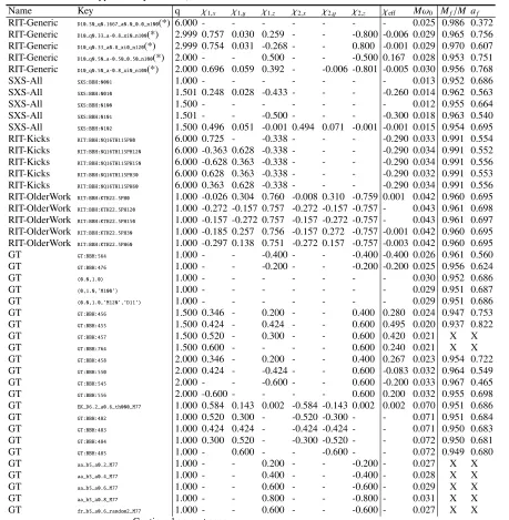
Our study makes use of 1139 distinct simulations of bi-nary black hole quasicircular inspiral and coalescence. Ta-ble II summarizes the salient features of this set: mass ratio and initial spins for the simulations used here, all initially in a quasicircular orbit with orbital separation along the ˆxaxis and velocities along±yˆ.

The RIT group provided 394 simulations [17, 27, 73]. The simulations include binaries with a wide range of mass ra-tios, as well as a wide range of black hole angular momentum (spin) magnitudes and directions [17, 27, 73, 74], including a simulation with large transverse spins and several spin pre-cession cycles which fits GW150914 well [27], as described below. The SXS group has provided both a publicly-available catalog of coalescing black hole binary mergers [75], a new catalog of nonprecessing simulations [76], and selected sup-plementary simulations described below. Currently extended

to 310 members in the form used here, this catalog includes many high-precision zero- and aligned-spin sources; selected precessing systems; and simulations including extremely high

black hole spin. The Georgia Tech group (GT) provided

406 simulations; see [15] and [77] for further details. This extensive archive covers a wide range of spin magnitudes and orientations, including several systematic one- and

two-parameter families. The Cardiff-UIB group provided 29

sim-ulations, all specifically produced to follow up GW150914 via a high-dimensional grid stencil, performed via the BAM code [78, 79]. These four sets of simulations explore the model space near the event in a well-controlled fashion. In addition to previously-reported simulations, several groups performed new simulations (108 in total) designed to reproduce the pa-rameters of the event, some of which were applied to our anal-ysis. These simulations are denoted in Table II and our other reports by an asterisk (*). These followup simulations include three independent simulations of the same parameters drawn from the distributions in LVC-PE[1], from RIT, SXS, and GT, allowing us to assess our systematic error. These simulations were reported in LVC-detect[2] and LVC-Burst[4], and are in-dicated by (+) in our tables.

The simulations used here have either been published pre-viously, or were produced using one of three well-tested procedures operating in familiar circumstances. For refer-ence, in Appendix A, we outline the three groups’ previously-established methods and results. For this application, we trust these simulations’ accuracy, based on their past track record of good performance. By incorporating simulations of identi-cal physics provided by different groups, our methods provide limited direct corroboration: simulations with similar physics produce similar results.

C. Directly comparing NR with data

For each simulation, each choice of seven extrinsic

param-eters θ (4 spacetime coordinates for the coalescence event;

three Euler angles for the binary’s orientation relative to the Earth), and each choice for the redshifted total binary mass

Mz=(1+z)M, we can predict the responsehkof both of the

k=1,2 LIGO instruments to the implied gravitational wave

signal. Usingλto denote the combination of redshifted mass

Mzand the numerical relativity simulation parameters needed to uniquely specify the binary’s dynamics, we can therefore evaluate the likelihood of the data given the noise:

lnL(λ;θ)=₋1

2

X

k

hhk(λ, θ)−dk|hk(λ, θ)−dkik− hdk|dkik,

(1)

wherehkare the predicted response of thekth detector due to a source with parametersλ, θ;dkare the detector data in instru-mentk; andha|bik ≡

R∞

−∞2d fa˜(f)∗b˜(f)/Sh,k(|f|) is an inner

product implied by thekth’s detector’s noise power spectrum

Sh,k(f); see, e.g., [80] for more details. In practice, as

-2 -1 0 1 2

-0.2 -0.15 -0.1 -0.05 0 0.05

Inspiral Merger Ringdown

Strain (10

-21

)

Time (seconds) H1 estimated strain, incident H1 estimated strain, band-passed

FIG. 1. Simulated waveform: Predicted strain in H1 for a source with parametersq=1.22, χ1,z =0.33, χ2,z =0.44, simulated in full general relativity; compare to Figure 2 in LVC-detect[2] . The gray line shows the idealized strain responseh(t) = F+h+(t)+F×h×(t),

while the solid black line shows the whitened strain response, using the same noise power spectrum as LVC-detect[2].

flow, so all inner products are modified to

ha_|b_ik≡2

Z

|f_|>flow

d fa˜(f) ∗b˜(f)

Sh,k(|f|)

. (2)

Except for an overall normalization constant and a different

choice for low-frequency cutoff, our expression agrees with

Eq. (1) in LVC-PE[1]. The joint posterior probability ofλ, θ

follows from Bayes theorem:

ppost(λ, θ)= L

(λ, θ)p(θ)p(λ)

R

dλdθ_L(λ, θ)p(λ)p(θ) , (3)

wherep(θ) andp(λ) are priors on the (independent) variables

θ, λ.1 _{For eachλ— that is, for each simulation and each}

red-shifted massMz— we evaluate the marginalized likelihood

Lmarg(λ)≡ Z

L(λ, θ)p(θ)dθ (4)

via direct Monte Carlo integration, where p(θ) is uniform in 4-volume and source orientation [80].2_{The marginalized}

like-lihood measures the similarity between the data and a source with parametersλand enters naturally into full Bayesian pos-terior calculations. In terms of the marginalized likelihood

and some assumed prior p(λ) on intrinsic parameters like

1_{For simplicity, we assume all black hole-black hole (BH-BH) binaries are}

equally likely anywhere in the universe, at any orientation relative to the detector. Future direct observations may favor a correlated distribution, including BH formation at higher masses at large redshift.

2_{Our choice for p(θ) differs only superficially from that adopted in}

LVC-PE[1], by adopting a narrower prior on the geocentric event time. Here, we allow±0.05 s around the time reported by the online analysis; LVC-PE[1] allowed±0.1 s.

masses and spins, the posterior distribution for intrinsic pa-rameters is

ppost(λ)=

Lmarg(λ)p(λ) R

dλLmarg(λ)p(λ). (5)

If we can evaluateLmargon a sufficiently dense grid of

intrin-sic parameters, Eq. (5) implies that we can reconstruct the full posterior parameter distribution via interpolation or other lo-cal approximations. This reconstruction needs to accurately

reproduce Lmarg only near its peak value; for example, if

Lmarg(λ) can be approximated by ad-dimensional Gaussian,

then we anticipate only configurationsλwith

lnLmax/_Lmarg(λ)> χ2_d,ǫ/2 (6)

contribute to the posterior distribution at the 1−ǫ credible interval, whereχ2_d,ǫis the inverse-χ2distribution.

Based on similarity of our distribution to a suitably-parameterized multidimensional Gaussian, we anticipate that only the region of parameter space with lnLmax−lnLmarg(λ).

6.7 can potentially impact our conclusions regarding the 90% credible level ford =8 (i.e., two masses and two precessing

spins); ford = 4, more relevant to the most strongly

acces-sible parameters (i.e., two masses and two aligned spins), the corresponding interval is lnLmax−lnLmarg(λ).4.

Each NR simulation corresponds to a particular value of seven of the intrinsic parameters (mass ratio and the three components of each spin vector) but can be scaled to an arbi-trary value of the total redshifted massMz. Therefore each NR simulation represents a one-parameter family of points in the 8-dimensional parameter space of all possible values ofλ. For each simulation, we evaluate the marginalized log likelihood versus redshifted mass lnLmarg(Mz) on an array of masses, adaptively exploring each one-parameter family to cover the interval lnLmax−lnLmarg(λ)<10. To avoid systematic bias

introduced by interpolation or fitting, our principal results are simply these tabulated function values, explored almost con-tinuously in massMzand discretely, as our fixed simulation archive permits, in other parameters. The set of intrinsic pa-rameters VC ≡ {λ : lnLmarg > C}above a cutoffC

iden-tifies a subset of binary configurations whose gravitational

wave emission is consistent with the data.3 _{Though this}

ap-proach provides a powerfully model-independent apap-proach to gravitational-wave parameter estimation, as described above it is restricted to the discrete grid of NR simulation values. For-tunately, the brevity and simplicity of the signal — only a few chirping and little-modulated cycles — requires the posterior

3_{While this approach works for multidimensional Gaussians, it can break}

distribution to be broad and smooth, extending over many nu-merical relativity simulations’ parameters. This allows us to go beyond comparisons on a discrete grid of NR simulations, and instead interpolate between simulations to reconstruct the entire distribution.

To establish a sense of scale, we can use a simple

order-of-magnitude calculation for lnLmarg. The signal to noise

ratio ρ and peak likelihood of any assumed signal are

re-lated: ρ = √2maxθlnL. Even at the best intrinsic

param-etersλ, the marginalized log-likelihood lnLmargwill be well

below the peak value maxθlnL, because only a small

frac-tion of extrinsic parameters θ have support from the data

[82]. Using GW150914’s previously-reported signal ampli-tude [ρ=23.5–26.8], its extrinsic parameters and their uncer-tainty [LVC-PE[1]], and our prior p(θ), we expect the peak

value of lnLmarg to be of order 240-330. The interval of

lnLmargselected by Eq. (6) is a small fraction of the full range

of lnLmarg, identifying a narrow range of parametersλwhich

are consistent with the data.

Our analysis of this event, as well as synthetic data,

sug-gests that lnLmargis often well-approximated by simple

low-order series in intrinsic parametersλ. This simple behavior is

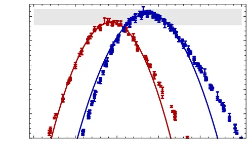
most apparent versus total mass Mz. Figure 2 shows

exam-ples of the marginalized log likelihood evaluated using two of our most promising simulation candidates: they are well-approximated by a quadratic over the entire observationally-interesting range. We approximate lnLmarg(Mz) as a second-order Taylor series,

lnLmarg(Mz)≃lnL− 1

2ΓM M(Mz−Mz,∗)

2_,

(7)

where the constants lnL,Mz,_∗, andΓM Mrepresent the largest value of lnLmarg, the redshifted mass at which this maximum

occurs, and the second derivative at the peak value. Even in (rare) cases when a locally quadratic approximation slightly

breaks down, we still use lnL to denote our estimate of the

peak of lnLmarg(Mz).4As a means of efficiently communicat-ing trends in the quality of fit versus intrinsic parameters, the two quantities lnLandMz,∗are reported in Table III.

Motivated by the success of this approximation, in Section

IV B we also supply a quadratic approximation to lnLmarg

near its peak,under the restrictive approximation that all an-gular momenta are parallel, using information from only non-precessing simulations. Using this quadratic approximation,

we can numerically estimate lnLmargand hence the posterior

[Eq. (5)] for arbitrary aligned-spin binaries. For any coordi-nate transformationz=Z(λ), we can use suitable supplemen-tary coordinates and direct numerical quadrature to determine the marginal posterior densityppost(z)=

R

ppost(λ)δ(z−Z(λ)).

As shown below, this procedure yields results comparable to LVC-PE[1] for nonprecessing binaries.

4_{We find similar results using more sophisticated nonparametric}

interpola-tion schemes. The results reported in Table III use one-dimensional Gaus-sian process interpolation to determine the peak value.

�� �� �� �� �� ��

��� ��� ��� ��� ��� ���

����_⊙�

��

ℒ��

��

FIG. 2. Likelihood versus mass: Examples: Raw Monte Carlo estimates for ln_Lmarg(Mz) versus Mz for two nonprecessing bina-ries: SXS:BBH:305 (blue) andd0 D10.52 q1.3333 a-0.25 n100

(red). To guide the eye, for each simulation we also overplot a local quadratic fit to the results near each peak. Results were evaluated withfmin=30 Hz; compare to Table III. Error bars reflect the stan-dard Monte Carlo estimate of the integral stanstan-dard deviation, multi-plied by 2.57 in the log to increase contrast (i.e., the nominal 99% credible interval, assuming the relative Monte Carlo errors are nor-mally distributed). To guide the eye, a shaded region indicates the interval of lnLmarg selected by our ansatz given a credible interval 90% and a peak value of ln_Lmargof 273; see Section III and Eq. (6).

D. Are there su_fficiently many and long NR simulations?

Because of finite computational resources, NR simulations of binary black holes cannot include an arbitrary number of orbits before merger. Instead, they start at some finite initial orbital frequency. While many NR simulations follow enough binary orbits to be compared with GW150914 over the en-tire LIGO frequency band, some NR simulations miss some early-time information. Therefore, in this section we describe a simple approximation (a low frequency cutoff) we apply to ensure that simulations with similar physics (but different ini-tial orbital frequencies) lead to similar results.

At the time of GW150914, the instruments had relatively poor sensitivity to frequencies below 30 Hz and almost no sensitivity below 20 Hz. For this reason, the interpretations

adopted in LVC-PE[1] adopted a low-frequency cutoff of

20 Hz. Because of the large number of cycles accumulated at low frequencies, a straightforward Fisher matrix estimate

[83, 84] suggests these low frequencies (20−30 Hz)

pro-vide a nontrivial amount of information, particularly about the binary’s total mass. Equivalently, using the techniques described in this paper, the function lnLmarg(Mz) will have a slightly higher and narrower peak when including all quencies than when truncating the signal to only include

fre-quencies above 30 Hz; see PE+NR-Methods[10].

Because of limited computational resources, relatively

few simulations start in a sufficiently wide orbit such

that, for Mz = 70M_⊙, their radiation in the most

LVC-PE[1]. If fmin is the low-frequency cutoff, Mω0/m .

0.02(Mz/70M_⊙)(fmin/20 Hz)(2/m), where Mω0 is the initial

orbital frequency of the simulation reported in Table II, can be safely used to analyze a signal containing a significant

contri-bution from themth harmonic of the orbital frequency.

Fig-ure 3 shows examples of the strain in LIGO-Hanford, pre-dicted using simulations of different intrinsic duration, su-perimposed with lines approximately corresponding to diff er-ent gravitational wave frequencies. To facilitate an apples-to-apples comparison incorporating the widest range of available simulations, in this work we principally report on compar-isons calculated by adopting a low-frequency cutoffof 30 Hz; see, e.g., Table III. (We also briefly report on comparisons

performed using a low-frequency cutoff of 10 Hz.) As we

describe in subsequent sections, while this choice of 30 Hz slightly degrades our ability to make subtle distinctions be-tween different precessing configurations, it does not dramati-cally impair our ability to reconstruct parameters of the event, given other significant degeneracies.

Even this generous low-frequency cutoff is not perfectly

safe: for each simulation, a minimum mass exists at which the starting gravitational wave frequency is 30 Hz or larger. In the plots and numerical results reported here, we have eliminated simulation and mass choices that correspond to scaling an NR simulation to a starting frequency above 30 Hz. The inclusion or suppression of these configurations does not significantly change our principal results.

This paper uses enough NR simulations to adequately sam-ple the four-dimensional space of nonprecessing spins, partic-ularly for comparable masses. As described below, this high simulation density insures we can reliably approximate the

marginalized likelihood lnLmarg for nonprecessing systems.

On the other hand, the eight-dimensional parameter space of precessing binaries is much more sparsely explored by the simulations available to us. But because the reconstructed gravitational wave signals in LVC-detect[2] and LVC-PE[1] exhibit little to no modulation, we expect that the remaining four parameters must have at best a subtle effect on the signal: the likelihood and posterior distribution should depend only weakly on any additional subdominant parameters. Having identified dominant trends using nonprecessing simulations, we can use controlled sequences of simulations with simi-lar parameters to determine the residual impact of transverse spins. Even if the marginalized likelihood cannot be safely approximated in general, a simulation’s value of lnLprovides insight into the parameters of the event.

Motivated by the parameters reported in LVC-PE[1] and our results in Table III, several followup simulations were performed to reproduce GW150914. These simulations are responsible for most of the best-fitting aligned-spin results re-ported in Table III.

E. Impact of instrumental uncertainty

For simplicity, our analysis does not automatically account for instrumental uncertainty (i.e., in the detector noise power spectrum or instrument calibration), as do the methods in

�� �� �� ��

���� ���� ���� ���� ���� ��� ���

��� �� � � ��

������� ��

����

��

��

�

FIG. 3.Best-fit detector response: A plot of the detector response (strain)h(t)=F+h+(t)+F×h×(t) evaluated at the LIGO-Hanford

de-tector , similar to Figure 2 in LVC-detect[2], Figure 6 in LVC-PE[1], and Figure 2 in LVC-TestGR[3], evaluated using two of the best-fitting numerical relativity simulations and total redshifted masses reported in Table III. The redshifted massesMzand extrinsic param-etersθnecessary to evaluate the detector response have been identi-fied using the methods used in this work and PE+NR-Methods[10], using alll=2 modes; a low-frequency cutoffof 30 Hz; and omitting the impact of calibration uncertainty. For comparison, the shaded region shows the 95% credible region for the waveform reported in LVC-PE[1], an analysis which accounts for calibration uncertainties and includes frequencies down to 20 Hz but approximates the radia-tion and omits higher harmonics (e.g, the (2,_±1) modes). To guide the eye, two vertical lines indicate the approximate time at which the signal crosses these two gravitational wave frequency thresholds.

LVC-PE[1]. LVC-PE[1] suggests that, for the intrinsic pa-rametersλof interest here, the impact of these systematic in-strumental uncertainties effects are relatively small. We have repeated our analysis using two versions of the instrumental calibration; we find no significant change in our results.

F. Comparison with other methods

LVC-Burst[4] reported on direct comparisons between

ra-diation extracted from NR simulations and

nonparametri-cally reconstructedestimates of the gravitational wave signal; see, e.g., their Fig. 12. Their comparisons quickly identified masses, mass ratios, and spins that were consistent with the data. Our study, which attempts a fully Bayesian direct com-parison between the data and the multimodal predictions of NR, produces results consistent with those of LVC-Burst[4]; see, e.g., Figure 4 described below.

model. To isolate the effects of NR, we have repeated our analysis but with the same nonprecessing waveform model used in LVC-PE[1] rather than with NR waveforms. Using the same input waveforms, our method and that of LVC-PE[1]

produce very similar results; see PE+NR-Methods[10] for

de-tails. To isolate the effects of the low-frequency cutoff, we performed the nonprecessing analysis reported in LVC-PE[1] with a low frequency cutoffof 30 Hz; we found results similar to LVC-PE[1].

IV. RESULTS I: PRE-COALESCENCE PARAMETERS

We present two types of results. For generic, precessing NR simulations, we evaluate the marginalized likelihood of source parameters given the data, but because the parameter-space coverage of NR simulations is so sparse, we do not at-tempt to construct an interpolant for the likelihood as a func-tion of source parameters. For nonprecessing sources, we con-struct such an interpolant, and we compare with the results of LVC-PE[1]. Using the computed likelihoods, we quan-tify whether the data are consistent with or favor a precessing source.

A. Results for generic sources, without interpolation

Because the available generic NR simulations represent only a sparse sampling of the parameter space, for generic sources we adopt a conservative approach: we rely only on our estimates of the marginalized likelihood lnLmarg, and we

do not interpolate the likelihood between intrinsic parameters, nor do we account for Monte Carlo uncertainty in each numer-ical estimate of lnLmarg. Using the inverseχ2distribution, we

identify two thresholds in lnLmarg using Eq. (6), one (our

preferred choice) obtained by adoptingd=4 observationally

accessible parameters, and the other adoptingd = 8.5 _Both

thresholds on lnLmargare derived using (a) our target credible

interval (90%) and (b) the peak log likelihood attained over all simulations [Table III]. Below, we find that the peak log likeli-hood over all simulations is lnLmarg=272.5; as a result, these two thresholds are lnLmarg = 268.6 and lnLmarg = 265.8,

for d = 4 and d = 8, respectively. The configurations of

masses and intrinsic parameters that pass either of these two thresholds are deemed consistent with the data. In subsequent figures, we will color these two classes of configurations in black (those configurations with lnLmarg > 268.6) and gray

(those configurations with lnLmarg >265.8). We use this set

of points in parameter space to bound (below) the range of parameters consistent with the data.

For the progenitor black hole parameters, our results using

l =2 modes are summarized in Figures 4 and 8 (for generic

5_{The second choice (d=8) would be appropriate if the posterior was}

well-approximated by an 8-dimensional Gaussian. The first choice (d=4) is motivated by past parameter estimation studies when the posterior distri-bution principally constrains the component masses and aligned spins.

sources), as well as by Figures 6 and 7 (for nonprecessing sources). For comparison, these figures also include the re-sults obtained in LVC-PE[1], using approximations appropri-ate for nonprecessing (black curves) and simply [18] precess-ing (blue curves) binaries. The first column of Table I shows the one-dimensional range inferred for each parameter by our

threshold-based method, usingl=2 modes only.

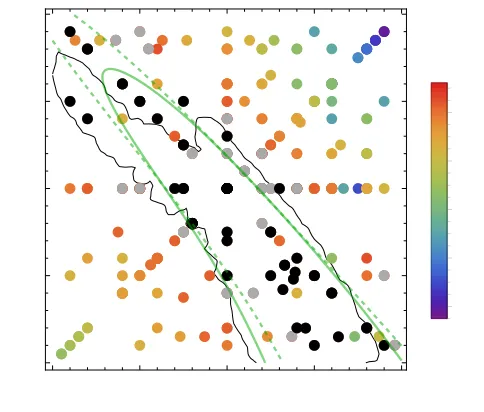
Before describing our results, we first demonstrate why our strategy is effective: Figures 4, 6, 7, and 8 show that the like-lihood is smooth and slowly varying, dominated by a few key parameters. As seen in the right panel of Figure 4, even our large NR array is relatively sparse. However, as the color scale on this and other figures indicate, the marginalized likelihood varies smoothly with parameters, over a range of more than

e100. The simplicity of lnLmarg is most apparent using con-trolled one- and two-parameter subspaces; for example, Fig-ure 6 shows that lnL (i.e., the peak of lnLmarg(Mz)) varies smoothly as a function ofχ1,z, χ2,zfor nonprecessing binaries of different mass ratiosq = m1/m2. Targeted NR

simula-tions have corroborated the simple dependence of the like-lihood seen here. Despite employing simulations with two strongly precessing spins and including higher harmonics, two factors which have been previously shown to be able to break degeneracies [24, 85–89], Table III reveals that simulations with the same values ofq andχeff almost always have

simi-lar values of lnL. In other words, these two simple parame-ters explain most of the variation inL, even whenLchanges by up to a factor ofe100_{. Finally and critically, simulations}

with similar physics produce very similar results. By adopt-ing flow=30 Hz and thereby largely standardizing simulation

duration, we find similar values of lnLwhen comparing the

data to simulations performed by different groups with simi-lar (or even identical) parameters.

Our results and that of LVC-PE[1] constrain the progenitor binary’s redshifted mass, mass ratio, and aligned effective spin

χeff; see Table I. The effective spin is defined as [90, 91]

χeff =(S1/m1+S2/m2)·Lˆ/M, (8)

For example, the color scale in Figure 4 provides a graphical representation of lnL versusχeff; large values of|χeff| (only

possible for spin-aligned systems) are inconsistent with the data. The agreement between our results and LVC-PE[1] per-sists despite using a much larger simulation set than those used to calibrate the models used in LVC-PE[1]; and de-spite employing simulations with black hole spins that are both precessing and with magnitude significantly outside the rangeχ < 0.5−0.8 for which these models were calibrated [11, 92, 93].

The three parameters Mz, q, and χeff are well-known to

have a strong and tightly-correlated impact on the gravita-tional wave signal and hence on implied posterior distribu-tions [82–84, 94, 95]. Since general relativity is scale-free, the total redshifted binary massMzsets the characteristic physical timescale of the coalescence. Due to strong spin-orbit cou-pling, aligned spins (χeff > 0) extend the temporal duration

post-- NR grid Aligned fit Overall LI NR grid (l_≤3) Aligned fit (l_≤3) Overall (l_≤3) Detector-frame initial total massMz(M⊙) 65.6–77.7 67.2 – 77.2 65–77.7 66–75 67.1–76.8 67.2.3–77.3 67.1–77.3

Detector-framem1,z(M⊙) 35–45 35–45 35–45 35–45 34.5–43.9 35–45 34.5–45

Detector-framem2,z(M⊙) 27–36 27–36.7 27–36.7 27–36 30–37.5 28–37 28–37.5

Mass ratio 1/q 0.66–1 0.62–1 0.62–1 0.62–0.98 0.67–1 0.69–1 0.67–1

Effective spinχeff -0.3 – 0.2 -0.2 – 0.1 -0.3–0.2 −0.24–0.09 -0.24 – 0.1 -0.2–0.1 -0.24–0.1

Spin 1a1 0–0.8 0.03–0.80 0–0.8 0.0–0.8 0–0.8 0.03–0.83 0–0.83

Spin 2a2 0–0.8 0.07–0.91 0–0.91 0.0–0.9 0–0.8 0.11– 0.92 0–0.92

Final total massMf,z(M⊙) 64.0–73.5 - 64.0– 73.5 63–71 64.2–72.9 64.2–72.9

Final spinaf 0.62–0.73 0.62– 0.73 0.60–0.72 0.62–0.73 0.62–0.73

TABLE I.Constraints onMz,q, χeff: Constraints on selected parameters of GW150914 derived by directly comparing the data to numerical relativity simulations. The first column reports the extreme values of each parameter consistent with ln_Lmarg>268.6 [Eq. (6), withd=4], corresponding to the black points shown in Figures 4, 7, and 10. These are computed using all thel = 2 modes of the NR waveforms. Because these extreme values are evaluated only on a sparse discrete grid of NR simulations, this procedure can underestimate the extent of the allowed range of each parameter. The second column reports the 90% credible interval derived by fitting ln_Lmargversus these parameters for nonprecessing binaries, to enable interpolation between points on the discrete grid inλ; see Section IV B for details. The third column is the union of the two intervals. For comparison, the fourth column provides the interval reported in LVC-PE[1], including precession and systematics. The remaining three columns show our results derived using alll_≤3 modes.

�� �� �� �� �� ��

���� ���� ��� ��� ���

����_⊙�

χ���

��� ��� ��� ��� ���

��� ��� ��� ��� ��� ���

���� ���� ��� ��� ���

���

χ���

��� ��� ��� ��� ���

FIG. 4. Mass, mass ratio, and effective spin are constrained and correlated: Colors represent the marginalized log likelihood as a function of redshifted total massMz, mass ratioqand effective spin parameterχeff. Each point represents an NR simulation and a particularMz. Points with 265.8 < lnLmarg < 268.6 are shown in light gray, with lnLmarg > 268.6 are shown in black, and with lnLmarg < 265.8 are shown according to the color scale on the right (points with ln_Lmarg<172 have been suppressed to increase contrast). Marginalized likelihoods are computed using flow = 30 Hz, using alll=2 modes, and without correcting for (small) Monte Carlo integral uncertainties. These figures include both nonprecessing and precessing simulations. For comparison, the black, blue, and green contours show estimated 90% credible intervals, calculated assuming that the binary’s spins and orbital angular momentum are parallel. The solid black contour corresponds to the 90% credible interval reported in LVC-PE[1], assuming spin-orbit alignment; the solid blue contour shows the corresponding 90% interval reported using the semianalytic precessing model (IMRP) in LVC-PE[1]; the solid green curve shows the 90% credible intervals derived using a quadratic fit to ln_Lmargfor nonprecessing simulations usingl=2 modes; and the dashed green curve shows the 90% credible intervals derived using ln_Lmargfrom nonprecessing simulations, calculated using all modes withl≤3; see Section IV B for details. Unlike our calculations, the black and blue contours from LVC-PE[1] account for calibration uncertainty and use a low frequency cutoffof 20 Hz.Left panel: Comparison forMz, χeff. This figure demonstrates the strong correlation between the total redshifted mass and spin. Right panel: Comparison forq, χeff. This figure is consistent with the similar but simpler analysis reported in LVC-Burst[4]; see, e.g., their Fig. 12.

merger quasinormal ringdown [97]. More extreme mass ratio extends the duration of the pre-merger phase while dramati-cally diminishing the amplitude and frequency of post-merger oscillations [67, 68, 98, 99]. As noted above, the data tightly constrain one of these combinations (e.g., the total redshifted

mass at fixed simulation parameters). Hence, our ability to constrain any individual parameterMz,q, orχeffis limited not

degeneracy between these tightly correlated parameters. Simulations with a variety of physics fit the data,

in-cluding strongly precessing systems. In Table III, several

simulations with large transverse spins but nearly zero net aligned spin fit the data almost as well as the best-fitting nonprecessing simulations (e.g., SXS:BBH:3; RIT simulation D10_q0.75_a-0.8_xi0_n100). As described below, Table V shows that these and other long precessing simulations fit even better when more low-frequency content is included.

The correspondence between our results and those pre-sented in LVC-PE[1] merits further reflection: by construction our fiducial analysis (Table III) omitted nontrivial early-time information (i.e.,f <30 Hz) which, for each simulation, more tightly constrains the range of masses that could be consistent with the data. In fact, as we show below, strong degeneracies in the gravitational wave signal between mass, mass ratio, and spin imply that our ability to break these degeneracies domi-nates our reconstruction of source parameters. Omitting infor-mation from low frequencies marginally reduces our ability to identify the range of masses that are consistent with the data

for one simulation; however, this omission does not impair our ability to draw conclusions overall, after accounting for uncertain spins and mass ratio.

Directly comparable to Fig. 12 in LVC-Burst[4], the right panel of Figure 4 provides a visual representation of one key correlation betweenqandχeff: only a narrow range of mass

ratios and aligned effective spinχeff are consistent with the

data. This range includes both nonprecessing and precessing simulations. Most other parameters have a subdominant ef-fect. For example, restricting attention to nonprecessing bina-ries for clarity, the data do not strongly discriminate between systems with similarχeffbut differentχ1,z, χ2,z; see, e.g., Fig-ure 6.

B. Results for nonprecessing sources, including interpolation

Both LVC-PE[1] and our highly-ranked simulations in Ta-ble III demonstrate that binary black holes with

nonprecess-ing spins can reproduce GW150914. Only four

parame-ters characterize a nonprecessing binary: the two

compo-nent massesm1,m2and the components of each BH’s

dimen-sionless spinχi projected perpendicular to the orbital plane (χ1,z, χ2,z). Nonprecessing binary black hole coalescences have been extensively simulated [45]; see, e.g., Table II. Sev-eral models have been developed to reproduce the leading-order gravitational wave emission (the (l,_|m_|)=(2,2) modes) [6, 8, 12, 57, 67, 68]; one, the SEOBNRv2 model [92], is adopted as a fiducial reference by LVC-PE[1]. While this model has not been calibrated to NR for large values ofχeff

and q [11], it has been shown to accurately reproduce the

(2,2) mode from binaries with comparable mass and low spins

[9, 11, 61]. Because of degeneracies, data from GW150914 do not easily distinguish between different points in param-eter space that have the same values of Mz,q, χeff; in

partic-ular, it is difficult to individually measureχ1,zandχ2,zwhen

q _≃ 1, χeff ≃ 0 and χ1,z ≃ −χ2,z; see, e.g., [95]. Because

GW150914 has comparable masses and is oriented face-off

with respect to the line of sight, even including higher-order modes in the gravitational waveform (which we do in our ap-proach here but is not done for the analytic waveform models) does not strongly break these degeneracies and allow us to distinguish individual spins.

By stitching together our fits for lnLmarg(Mz) and recon-structing the relevant parts of the likelihood for all masses and aligned spins, we can estimate the full posterior distribution for Mz,q, χ1,z, χ2,z using Eq. (5). Due to inevitable system-atic modeling errors in the fit, as described below, this ap-proximation may not have the statistical purity of the method presented in LVC-PE[1]: any credible intervals or deductions drawn from it should be interpreted with judicious

skepti-cism. On the other hand, this method enables the reader

to recalculate the posterior distribution using any priorp(λ), including astrophysically-motivated choices. Fitting to non-precessing simulations, we find lnLmarg for lnLmarg > 262

is reasonably well-approximated by a quadratic function of the intrinsic parametersMz = (m1,zm2,z)3/5/(m1,z+m2,z)1/5, η =(m1,zm2,z)/(m1,z+m2,z)2,δ =(m1,z−m2,z)/Mz,χeff, and

χ₋≡(m1,zχ1−m2,zχ2)·Lˆ/Mz:

lnLmarg≃268.4−1

2(λ−λ∗)aΓab(λ−λ∗)b−Γχ−δχ−δ.(9a)

where the indicesa,b run over the variablesMz, η, χeff, χ₋.

In this expression,λa represents the vector (Mz, η, χeff, χ₋),

λ_∗a corresponds to the vector (Mz = 31.76M⊙,η = 0.255,

χeff = −0.037, χ₋ = 0) of parameters which maximize

lnLmarg, andΓis a matrix (indexed byMz, η, χeff, χ₋, δ) with

numerical values Γ =                  

3.75 −224.2 −52.0 0 0

−224.2 22697.2 2692 0 0

−52.0 2692. 846.9 0 0

0 0 0 2.57 −16.3

0 0 0 −16.3 0

                  . (9b)

Here we retain many significant digits to account for structure inΓ, which is nearly singular. Equation (9) respects exchange symmetrym1,z, χ1 ↔ m2,z, χ2. Our results do not sensitively

depend on the value ofΓχ−,χ−, indicating that this quantity is

not strongly constrained by the data. Conversely, the posteri-ors do depend onΓχ−,δ. As the contrast between the first term

in Eq. (9) and the data Table III makes immediately appar-ent, this coarse approximation can differ from the simulated results by of order 1.7 in the log (rms residual). This reflects the combined impact of Monte Carlo error, systematic error caused by too few orbits in some simulations, and system-atic errors caused by sparse placement of NR simulations and non-quadratic behavior of lnLmargwith respect to parameters.

Repeating our calculation while including all thel_≤3 modes, we find the same functional form as Eq. (9), but with a dif-ferent vectorλ(3)_∗,a=(Mz = 38.1M_⊙,η ≃ 0.32, χeff = 0.11,

χ₋=0), and a different matrix

Γ(3)=

                 

3.746 −235.5 −51.5 0 0

−235.5 17970 2941 0 0

−51.5 2941 833.2 0 0

0 0 0 0.57 −12.57

0 0 0 −12.57 0

�� �� �� �� �� �� �� ���� ���� ���� ���� ���������� ��_⊙� �� �� � ��� ��� ��� ��� ��� ��� ��� ��� ��� ��� ��� ��� ��� ��� ��� �� �� �� �� � ���� ���� ��� ��� � � � � � � χ��� �� ��

χ���

FIG. 5.Distributions agree [nonprecessing case]: Comparison between the posterior distributions reported in LVC-PE[1] for nonprecessing binaries (solid) and the posterior distributions implied by a leading-order approximation to lnLmarg[Eq. (9)] derived usingl≤2 (dotted) and

l_≤3 (dashed).Left panel:m1,z(black) andm2,z(red).Center panel: Mass ratio 1/q=m2,z/m1,z. The data increasingly favor comparable-mass

binaries as higher-order harmonics are included in the analysis.Right panel: Aligned effective spinχeff. The noticeable differences between ourχeffdistributions and the solid curve are also apparent in Figures 7 and 4: our analysis favors a slightly higher effective spin.

���� ���� ���� � ��� ��� ��� ���� ���� ��� ��� ��� ���� ���� ��� ��� ���

χ� �

χ�� �������� ���� ���� ���� � ��� ��� ��� ���� ���� ��� ��� ��� ���� ���� ��� ��� ���

χ� �

χ�� �������� ���� ���� ���� � ��� ��� ��� ���� ���� ��� ��� ��� ���� ���� ��� ��� ���

χ� �

χ�� �������� ��� ��� ��� ��� ���

FIG. 6.Likelihood versus spins: Nonprecessing: Maximum likelihood lnL(colors, according to the colorbar on the right) as a function of spinsχ1,z, χ2,zfor different choices of mass ratio 1/q, computed using alll=2 modes. Each point represents a nonprecessing NR simulation from Table III. To increase contrast, simulations with lnL <171 have been suppressed. Only simulations with fstart <30 Hz are included. Dashed lines and labels indicate contours of constantχeff. The left two panels show that for mass ratioq≃1, the marginalized likelihood is approximately constant on lines of constantχeff. For more asymmetric binaries (q=2), the marginalized likelihood is no longer constant on lines of constantχeff. Along lines of constantχeffandq, lnLdecreases versusχ2,z

We labelλ(3)_andΓ(3)_{with a superscript “3” to distinguish this}

result from the corresponding result using onlyl =2 modes

shown in Eq. (9).

For nonprecessing sources, using Eq. (5) and a uniform prior inχ1,z, χ2,zand the two component masses, we can eval-uate the marginal posterior probability p(z) for any intrinsic

parameter(s)z. The two-dimensional marginal posterior

prob-ability is shown as a green solid (l=2) and dashed (l_≤3) line

in Figures 4 and 7. Both thel=2 andl_≤3 two-dimensional

distributions are in reasonable agreement with the posterior distributions reported in LVC-PE[1] for nonprecessing bina-ries, shown as a black curve in these figures. These two-dimensional distributions are also consistent with the dis-tribution of simulations with lnLmarg > 268.6 (i.e., black

points). Additionally, Figure 5 shows several one-dimensional marginal probability distributions (m1,z,m2,z,q, χeff), shown as

dotted (l=2) or dashed lines (l≤3); for comparison, the solid line shows the corresponding distribution from LVC-PE[1] for nonprecessing binaries.

Despite broad qualitative agreement, these

compar-isons highlight several differences between our results and

LVC-PE[1], and between results includingl =2 modes and

those including alll≤3 modes. For example, Figure 4 shows

that the distribution inMz,q, χeff, computed using our method

(solid green lines and black points) is slightly different than the corresponding distributions in LVC-PE[1]. As seen in this figure and in Figure 7, the posterior distribution in LVC-PE[1] includes binaries with low effective spin, outside the support of the distributions reported here. These differences are di-rectly reflected in the marginal posterior p(χeff) (right panel

of Figure 5) and in Table I. Our results for the component spinsχ1,z, χ2,z, the effective spinχeff, the total massMz, and the mass of the more massive objectm1,zdo not change

sig-nificantly when l = 3 modes are included. The mass ratio

distribution p(q) is also slightly different from LVC-PE[1]

when l = 3 modes are included; see Figure 5. Compared

���� ���� ��� ��� ��� ����

���� ��� ��� ���

χ�� χ��

��� ��� ��� ��� ���

FIG. 7. Aligned spin components not constrained [aligned only shown]: Colors represent the marginalized log likelihood as a func-tion of the aligned spin componentsχ1,z and χ2,z. Each point

rep-resents an NR simulation; only nonprecessing simulations are in-cluded. Points with 265.8 < lnL < 268.6 are shown in light gray, with lnL >268.6 are shown in black, and with lnL <265.8 are shown according to the color scale on the right (points with ln_Lmarg < 172 have been suppressed to increase contrast). [The quantity lnLis the maximum value of ln_Lmargwith respect to mass; see Eq. (7).] Consistent with our other results, flow = 30 Hz. For comparison, the solid black contours show the 90% credible intervals derived in LVC-PE[1], assuming spin-orbit alignment and omitting corrections for waveform systematics. The solid and dashed green contours are the nominal 90% credible interval derived using an ap-proximation to our data for ln_Lmarg, assuming both spins are exactly parallel to the orbital angular momentum, forl=2 (solid) andl=3 (dashed), respectively; see Section IV B for more details.

Figure 5.

The differences between the results reported here and

LVC-PE[1] should be considered in context: not only does our study employ numerical relativity without analytic wave-form models, but it also adopts a slightly different starting frequency, omits any direct treatment of calibration uncer-tainty, and employs a quadratic approximation to the likeli-hood. That said, comparisons conducted under similar lim-itations and using real data, differing only in the underlying

waveform model, reproduce results from LALInference; see

PE+NR-Methods[10] for details.

By assuming the binaries are strictly aligned but permitting generic spin magnitudes, our analysis (and that in LVC-PE[1]) neglects prior information that could be used to significantly influence the posterior spin distributions. For example, the part of the posterior in the bottom right quadrant of Figure 7 is unstable to large angle precession [100]: if a comparable-mass binary formed at large separation with χ1,z > 0 and χ2,z<0, it could not remain aligned during the last few orbits. Likewise, the astrophysical scenarios most likely to produce strictly aligned binaries — isolated binary evolution — are most likely to result in bothχ1,z, χ2,z>0: both spins would be

strictly and positively aligned (see, e.g, [101]). In that case, only the top right quadrant of Figure 7 would be relevant. Us-ing the analytic tools provided here, the reader can regenerate approximate posterior distributions employing any prior as-sumptions, including these two considerations.

C. Transverse and precessing spins

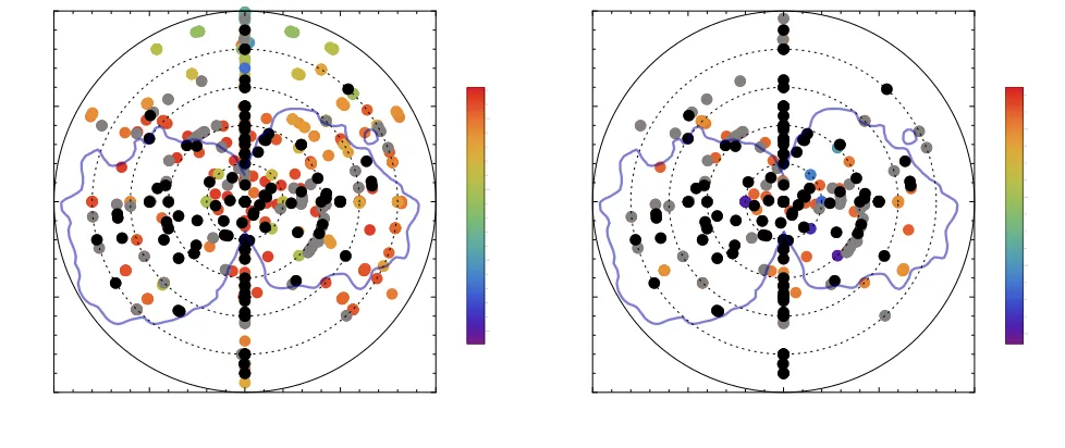
Figure 8 shows the maximum likelihood for the available NR simulations, plotted as a function of the magnitude of the aligned and transverse spin components. The figure shows that there are both precessing and nonprecessing simulations that have large likelihoods (black points), indicating that many precessing simulations are as consistent with the data as non-precessing simulations. Moreover, simulations with large pre-cessing spins are consistent with the GW150914: many con-figurations haveχeff ≃0 but large spins on one or both BHs in

the binary. Keeping in mind the limited range of simulations available, the magnitude and direction of either BHs spin can-not be significantly constrained by our method.

Not all precessing simulations with suitableq, χeffare

con-sistent with GW150914; some have values of lnL that are

not within 10 of the peak; see the right panel of Fig. 8) The marginal log-likelihood lnLdepends on the transverse spins, not just the dominant parameters (q, χeff,Mz). As a concrete illustration, Figure 9 shows that the marginalized log likeli-hood depends on the specific direction of the transverse spin, in the plane perpendicular to the angular momentum axis. Specifically, this figure compares the peak marginalized log likelihood (lnL) calculated for each simulation with the value of lnLpredicted from our fit to nonprecessing binaries. For precessing binaries, lnLis neither in perfect agreement with the nonprecessing prediction, nor independent of rotations of the initial spins about the initial orbital angular momentum by an angleφ.

While the transverse spins do influence the likelihood, slightly, the data do not favor any particular precessing con-figurations. No precessing simulations had marginalized like-lihoods that were both significant overall and significantly above the value we predicted assuming aligned spins. In other words, the data do not seem to favor precessing systems, when analyzed using only information above 30 Hz.

Our inability to determine the most likely transverse spin components is expected, given both our self-imposed restric-tions (flow =30 Hz) and the a priori effects of geometry. For

example, the lack of apparent modulation in the signal re-ported in LVC-detect[2] and LVC-Burst[4] points to an

ori-entation with J parallel to the line of sight, along which

precession-induced modulations are highly suppressed. In ad-dition, the high mass and hence extremely short observation-ally accessible signal above 10 Hz provides relatively few cy-cles with which to extract this information. The timescales involved are particularly unfavorable to attempts to extract precession-induced modulation from the pre-merger signal: the pre-coalescence precession rate for these sources is low (Ωp ≃(2+3m2/m1)J/2r3 ≃2π×1 Hz(f/40 Hz)5/3for this