This is a repository copy of
Dummy coding vs effects coding for categorical variables:
clarifications and extensions
.
White Rose Research Online URL for this paper:
http://eprints.whiterose.ac.uk/104911/
Version: Accepted Version
Article:
Daly, A orcid.org/0000-0001-5319-2745, Dekker, T orcid.org/0000-0003-2313-8419 and
Hess, S orcid.org/0000-0002-3650-2518 (2016) Dummy coding vs effects coding for
categorical variables: clarifications and extensions. Journal of Choice Modelling, 21. pp.
36-41. ISSN 1755-5345
https://doi.org/10.1016/j.jocm.2016.09.005
© 2016 Elsevier Ltd. All rights reserved. This manuscript version is made available under
the CC-BY-NC-ND 4.0 license http://creativecommons.org/licenses/by-nc-nd/4.0/
[email protected] https://eprints.whiterose.ac.uk/ Reuse
Unless indicated otherwise, fulltext items are protected by copyright with all rights reserved. The copyright exception in section 29 of the Copyright, Designs and Patents Act 1988 allows the making of a single copy solely for the purpose of non-commercial research or private study within the limits of fair dealing. The publisher or other rights-holder may allow further reproduction and re-use of this version - refer to the White Rose Research Online record for this item. Where records identify the publisher as the copyright holder, users can verify any specific terms of use on the publisher’s website.
Takedown
If you consider content in White Rose Research Online to be in breach of UK law, please notify us by
Dummy coding vs effects coding for categorical variables: clarifications and extensions
Andrew Daly – Thijs Dekker – Stephane Hess
Institute for Transport Studies & Choice Modelling Centre - University of Leeds
VERSION ACCEPTED FOR PUBLICATION IN JOURNAL OF CHOICE MODELLING ON 04/09/2016
Abstract
This note revisits the issue of the specification of categorical variables in choice models, in the context of ongoing discussions that one particular normalisation, namely effects coding, is superior to another, namely dummy coding. For an overview of the issue, the reader is referred to Hensher et al. (2015, see pp. 60-69) or Bech and Gyrd-Hansen (2005). We highlight the theoretical equivalence between the dummy and effects coding and show how parameter values from a model based on one normalisation can be transformed (after estimation) to those from a model with a different normalisation. We also highlight issues with the interpretation of effects coding, and put forward a more well-defined version of effects coding.
Keywords: dummy coding; effects coding; discrete choice; categorical variables
1. Introduction
Choice models describe the utility of an alternative as a function of the attributes of that alternative. Those attributes might be continuous or categorical, where the simplest example of the latter is a binary present/absent attribute. In the case of continuous attributes, the associated coefficient (say ) measures the marginal utility of changes in the attribute (say x), and the analyst simply needs to make a decision on whether that marginal utility is independent of the base level of the attribute (i.e. linear) or not (i.e. non-linear). For the latter, we would simply replace in the utility function with , where is a non-linear transformation of .
Just as for continuous attributes, an analyst needs to make a decision on how categorical variables are treated in the computation of an alternative’s utility. For continuous variables, it is clear that different assumptions in terms of functional form (linear vs non-linear, and the specific degree of non-linearity) will lead to different model fit and behavioural implications. However, in the case where is a categorical variable with a finite number of different levels, neither a linear nor a function-based non-linear treatment is likely to be appropriate. With taking the values for the different levels it can assume, a linear treatment would imply that the difference in utility between successive levels are equal. The fundamental differences in meaning of different levels of categorical variables may also make it difficult for an analyst to find an appropriate functional form for in a non-linear specification.
For categorical variables, model estimation captures the impact on utility of moving from one level of the attribute to a different level. Because of linear dependency, it is then impossible to estimate a separate parameter for each level. Different approaches have been put forward in the literature to address this issue, in particular dummy coding and effects coding, although many other approaches would be possible. The purpose of this note is to address ongoing discussions in the choice modelling literature which claim that some of the ways of dealing with such variables (in particular effects coding) are superior to others. For an overview of the issue, the reader is referred to Hensher et al., (2015, see pp. 60-69) or Bech and Gyrd-Hansen (2005).
2. Equivalence and interchangeability of dummy and effects coding of categorical variables
variables for alternative j, say , with , where, for a given alternative , , if , and 0 otherwise. It is important to stress that this applies both in the case of labelled alternatives, where e.g. may refer to a given mobile phone model, or unlabelled alternatives, where e.g. may refer to whether an alternative is presented on the left hand side in a survey. Not including ASCs is equivalent to an assumption that the means of the error terms, including unmeasured variables, are identical across alternatives. With this notation, the contribution of the ASC component to the utility of alternative j would now be given by , where, for any given alternative j, only one element in , with
, will be equal to 1 (and all others will be 0).
It is then widely known that a restriction has to be imposed to make the model identifiable, i.e. it is impossible to estimate a value , where . This is a result of the fact that probabilities in choice models are defined in terms of utility differences across the J alternatives in the consumer’s choice set, and an infinite number of combinations of values for the ASCs would lead to the same differences. A constraint needs to be applied to avoid linear dependency and thereby make the model identifiable. A typical approach in this context is to set the ASC for one alternative (e.g. the last) to zero, e.g. , and estimate the remaining ones, i.e. . As we will see later on, this is in effect using dummy coding for the ASCs, with the value of one ASC set to 0 and all others being estimated.
While the use of dummy coding for ASCs is commonplace, substantial discussion has gone into the appropriate specification to use for other categorical variables, which are our main focus. Let us consider, for example, the case of a categorical variable for alternative j, say , where we assume that this variable has K different levels (i.e. possible values)1. In the absence of an acceptable assumption about some continuous relationship between the different levels of and the utility of alternative j, we are then in a situation where we want to estimate independent different utility components for its different levels. This leads to the need for recoding and/or, as mentioned above, for some constraints to be imposed on the specification. The key distinction made in the literature has been between dummy coding and effects coding. We will now illustrate how these can be arrived at through different ways of recoding the categorical variable. The rationale behind recoding is that we create a number of separate variables for the separate levels of each categorical variable, where different parameters are associated with the resulting variables.
Table 1 presents the way in which a four-level categorical variable would typically be recoded into dummy and effects coding (see also Hensher et al. (2015, see pp. 60-69) or Bech and Gyrd-Hansen (2005)). With either approach, we recode the categorical variable x into four new variables, which each have an associated parameter, i.e. for the dummy-coded variables or, in the alternative model specification, for the effects-coded variables.
When adopting either of these coding conventions, we can without loss of generality normalise the parameter of the fourth (last) level to zero for identification purposes.2 We thus estimate three parameters with either approach. The difference arises in the final level of x. For the first K-1 levels, one recoded variable is equal to 1 (e.g. with the first level, for dummy coding and for effects coding), while all others are zero. However, while this is still the case for the final level of x also for dummy coding, with effects coding, we additionally set the values for the first K recoded variables to -1. The utility contribution K,D associated with level K under dummy coding is then zero since , while, under effects coding K,E= , i.e. the negative sum of all the estimated effects coded parameters (remembering that . The sum of utility contributions across all K levels is thus zero with effects coding and this is the objective of effects coding.
1Similar coding procedures would also be applicable when linearly dependent variables occur across alternatives,
but for simplicity we focus here on the case of variables applying for a single alternative.
2 In dummy coding correlations between the parameters can be minimised by selecting the base category to be the
The first point that we wish to make in this paper is that while the approach described above is the
‘standard’ way of understanding effects coding in much of the literature, the recoding itself is not required. Indeed, a completely equivalent approach would be to retain the dummy coded variables but, instead of setting , we could use a normalisation that . This would then give us
that , and . In short, the two alternative recoding approaches are
identical, but rely on alternative normalisations. The recoding typically applied when analysts use effects coding is thus not required. Should we wish to have effects coded parameters, we can just recode the categorical variable into K binary 0-1 variables as in dummy coding, and impose the constraint
.
Table 1: Illustrative example
Dummy coding Effects coding
Recoded variables Utility
contribution (
Recoded variables Utility
contribution (
Level of
1 1 0 0 0 1 0 0 0
2 0 1 0 0 0 1 0 0
3 0 0 1 0 0 0 1 0
4 0 0 0 1 0 -1 -1 -1 1
associated parameter
Moving away from the issue of recoding of variables, our next point relates to the equivalence between the two approaches. The above discussion highlights that the utility contribution of dummy and effects coding differs up to a constant, i.e. . The latter term drops out when taking differences across levels leaving the utility difference between any two categories unchanged.
for
When level K is not contrasted then we get for . This directly
follows from the utility contributions in Table 1. More important, we can use the contrast with level K to establish the correspondence between the two coding schemes.
where is the dummy-coded parameter for category is the effects-coded parameter for or category
is the utility associated with category k under dummy coding, with a corresponding definition for under effects coding
is the number of categories.
Adding these relationships for all of the categories except , we obtain
so
approach in estimation and then transform the estimates after estimation to the values that would have been obtained with a different approach, and use the Delta method (cf. Daly et al, 2012) to compute the associated standard errors. This directly refutes the notion that one recoding approach is inferior a priori or prevents an analyst from gaining particular insights after estimation.
This now brings us to a key argument put forward by advocates of effects coding in the literature, namely that of confounding between dummy coded ASCs and dummy coded categorical variables. Let us consider the simple example of a choice between two types of mobile phone, say from company A and company B. Let us further assume that these two phones are described on the basis of cost (which is treated continuously), screen size (4, 5 and 6 inches) and connectivity (3G, 4G, 4G+wifi). Assuming that we would use dummy coding for the ASCs (as is commonly done), we would estimate the parameters in Table 2 from our model with the two coding approaches for the categorical variables.
Table 2: Illustrative example 2
Brand
Price Screen size Connectivity
A B 4” 5” 6” 3G 4G 4G+wifi
Dummy coding for screen
and connectivity 0 0 0
Effects coding for screen
and connectivity 0
-We know from the earlier discussion that both specifications will give exactly the same model fit to the data, but the actual parameter estimates will differ between the two specifications. The argument put forward by advocates of effects coding is that with dummy coding, there is confounding between the base level for the dummy coded ASC and the base levels for the dummy coded categorical variables, as well as between the base levels for the individual dummy coded categorical levels. It is indeed true
that with the above, we have that , while it is quite likely that
. An interpretation used in some literature is that, in dummy coding, we then do not know whether it is better (or worse) to have brand A, or a screen size of 6 inches, or a phone with 4G and wifi. However, this misses the crucial point that only differences in utility matter, in comparisons between alternatives and also between values for a given attribute. What matters is not the absolute contribution of say to the utility, but the change in utility say for moving from a 5-inch screen to a 6-inch screen, and how that compares to moving from brand A to brand B. From the above theoretical discussions, we know that the differences in utility between individual levels for a given variable are not affected by which normalisation is used, and as a result, this confounding does not actually matter. More importantly, as we will see in the next section, the values obtained for a given level in effects coding are a function of the specification used for that effects coding. With the dummy coding above, the estimate for say would give us the value for a five inch screen relative to a six inch screen, while, with effects coding, gives the value of a five inch screen relative to the unweighted average of all the categories. The estimate for is thus not reference free either. In Section 4, we will investigate whether different specifications may yield more stable reference points.
3. Interpretation of effects coding
We saw above that, irrespective of the selected approach, only additional parameters can be estimated to avoid linear dependencies in the model3. However, another question that arises in choosing an approach is the usefulness of the outputs. In what follows, we move away from the discussion about confounding highlighted at the end of the previous section, and attempt to gain insights into the specific nature of the estimates from models with effects coding.
3 This restriction on the number of parameters applies to estimating the main effects on the utility of an alternative.
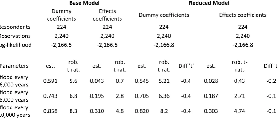
The model shown in Table 3 is a simple example based on the dataset used in Dekker et al. (2016) where a Dutch online panel of 224 respondents was presented with alternative flood risk reduction policies mitigating the future impact of climate change in the Netherlands. Key attributes were flood risk probability (four levels equally spaced between 1/4,000 years to 1/10,000 years), percentage of compensation received after a flood (0%, 50%, 75% and 100%), available evacuation time (6, 9, 12 and 18 hours) and increases in taxes to the local water authority (€0, €40, €80, €120 and €160). Each respondent answered 10 choice tasks where two policy options where contrasted with the status quo option. The status quo option took the following levels: (1/4,000 years, 0%, 6 hours and €0 additional tax). The presented policy options all provide an improvement relative to the do nothing (status quo) scenario in the non-cost attributes, but an increase in cost (so €0 does not apply). A D-efficient experimental design was used to choose the combinations of improvements in non-cost attribute levels and the increase in cost for the policy options. Apart from the €0 cost level, the D-efficient experimental design used all possible attribute levels to construct policy options as long as they provided an improvement over the ASC.4No status quo ASC is estimated as the €0 cost level is specific to the status quo alternative.
[image:6.595.74.522.500.717.2]With this data, the base value for cost (€0) applies only to the status quo alternative, and the estimation of values for the other four levels thus preclude the estimation of an ASC. The coefficient estimates shown in the first columns of the table, headed ‘Base Model’, for dummy coding and effects coding illustrate that the differences between given levels for a given attribute are the same across the two coding types. Moreover, the models are identical in the probabilities that they generate for each observation and then of course the overall likelihood is the same. In these models the coefficient for the first level of the attribute does not appear, as it is used as the base; in the dummy-code version this coefficient is zero, while in the effects-code version the coefficient is equal to minus the sum of the other coefficients for that attribute. Returning briefly to the notion in the literature about confounding, a comparison of say the estimates for “flood ever 10,000 years” between the two models is not informative – for dummy coding, the estimate of 0.858 is the difference to the base level of a flood every 4,000 years, while, for effects coding, the estimate of 0.310 is the value relative to the unweighted average of all four levels. However, we confirm that the differences across levels within a given attribute are constant, the arguments towards the end of Section 2 thus apply, and there is no confounding in either specification of the model.
Table 3: Estimates of base and reduced model
Base Model Reduced Model
Dummy coefficients
Effects
coefficients Dummy coefficients Effects coefficients
Respondents 224 224 224 224
Observations 2,240 2,240 2,240 2,240
Log-likelihood -2,166.5 -2,166.5 -2,166.8 -2,166.8
Parameters est. rob.
t-rat. est.
rob.
t-rat. est.
rob.
t-rat. Diff 't' est.
rob.
t-rat. Diff 't'
flood every
6,000 years 0.591 5.6 0.043 0.7 0.545 5.21 -0.4 0.028 0.43 -0.2
flood every
8,000 years 0.743 6.8 0.195 2.8 0.705 6.36 -0.4 0.187 2.71 -0.1
flood every
10,000 years 0.858 8.3 0.310 4.8 0.820 8.2 -0.4 0.303 4.74 -0.1
4 It should be noted that the obtained dummy / effects coded parameters are point estimates of recoded continuous
50%
compensation 0.586 5.5 -0.046 -0.8 0.543 5.1 -0.4 -0.063 -1.02 -0.3
75%
compensation 0.857 7.6 0.225 3.6 0.830 7.75 -0.2 0.224 3.61 0.0
100%
compensation 1.085 8.6 0.453 6.7 1.053 8.4 -0.3 0.446 6.55 -0.1
9 hours
evacuation time 0.223 2.1 0.017 0.2 0.187 1.93 -0.3 0.007 0.09 -0.1
12 hours
evacuation time 0.251 1.9 0.045 0.5 0.211 1.69 -0.3 0.031 0.38 -0.2
18 hours
evacuation time 0.350 3.4 0.144 2.1 0.321 3.42 -0.3 0.141 2.1 0.0
-0.109 -0.7 0.488 6.8
-0.214 -1.77 n.a. 0.429 5.67 n.a.
-0.304 -1.7 0.293 3.5
-0.998 -5.7 -0.401 -5.8 -0.900 -7.94 0.6 -0.256 -4.59 -3.5
-1.574 -8.3 -0.977 -10.7 -1.460 -10.9 0.6 -0.816 -9.9 2.1
For effects coding, it is then often implied that indicates the utility of the k-th level on some cardinal scale, but we must ask what the zero of this scale represents. The answer is given by the
constraint , i.e. . Therefore, can be interpreted as giving the
difference in utility between and the unweighted average of all the categories. Note that this applies to category also.
However, this ‘zero’ is ultimately not well defined. This is illustrated in the ‘Reduced Model’ in Table 3, where the coefficients for cost levels 2 and 3, which were similar in the base model, have been constrained to be the same. Again, the dummy-coded and effects-coded versions are identical, yielding a likelihood value reducing from –2166.50 to –2166.83 which indicates (through a test for one degree of freedom) that the merging of the coefficients does not significantly impact the fit to the data. The column headed “Diff. ‘t’” indicates the change in the coefficient value relative to the base model compared with the estimation error in the base mode coefficient. Here we see that none of the coefficients in the dummy-coded model have changed significantly, but the coefficients for the unaffected levels of the cost attribute in the effects-coded model have indeed changed significantly. The impact of a given level of an attribute relative to this zero thus depends on the way in which other levels of the attribute are coded. It seems that the interpretation of effects coding is not quite what is intended. While there is no confounding, the interpretation of the meaning of the effects codes is uncertain.
This uncertainty of meaning can be eliminated by a redefinition of the way in which effects codes are defined, but the values do not become reference free.
4. Well-defined effects coding
The key problem in standard effects coding is that the constraint on the codes is applied without considering the relative importance of the categories involved. An alternative is to consider a weighted coding, i.e.
instead of , consider
where is the share observed for category . This approach relates to a simple ANOVA on unbalanced data, where it is also known as Type 1 Sum of Squares or sequential sum of squares (Herr, 1986, Shaw and Mitchell-Olds, 1993).
To obtain this improved specification for effects coding, it is necessary to redefine the constraint, so
that instead of we specify . When a category is merged,
population-weighted average instead of the category-population-weighted average. This change may be seen to help in comparing values across different categorical variables, as they are estimated relative to a stable base, however, the crucial point is that the estimates still refer to a base.
Introducing changes the equations relating and
Adding these relationships multiplied by for all of the categories except , we obtain
so
A practical procedure would be to estimate , then derive , taking advantage of the fact that dummy coding is slightly easier to set up than effects coding. The calculation could then use weights that can be adjusted to meet different estimates of the population. For example, a model may be developed from a sample that is deliberately biased to focus on population segments of particular interest, but the coefficients could then be adjusted to give better representation of the whole population.
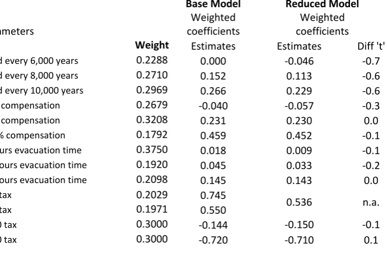
[image:8.595.96.473.508.754.2]The way in which this recoding would impact on the model of Table 3 is shown in Table 4 – these values are obtained through calculations, no re-estimation is needed, using the final equation given above to make the calculations. The first column of the table gives the weights that have been used, in this case the shares of the SP sample with each value of the attribute. The second column shows the weighted effects-coding coefficients, i.e. relative to the population mean. The third column shows the weighted effects-coded coefficients for the reduced model, while the final column presents a ‘t’ test of the hypothesis that the values are unchanged. In this case we see that the unaffected cost coefficients have not changed significantly, since they are measured relative to the fixed overall mean value.
Table 4: Weighted effects coding
Base Model Reduced Model
Parameters
Weighted coefficients
Weighted coefficients
Weight Estimates Estimates Diff 't'
flood every 6,000 years 0.2288 0.000 -0.046 -0.7
flood every 8,000 years 0.2710 0.152 0.113 -0.6
flood every 10,000 years 0.2969 0.266 0.229 -0.6
50% compensation 0.2679 -0.040 -0.057 -0.3
75% compensation 0.3208 0.231 0.230 0.0
100% compensation 0.1792 0.459 0.452 -0.1
9 hours evacuation time 0.3750 0.018 0.009 -0.1
12 hours evacuation time 0.1920 0.045 0.033 -0.2
18 hours evacuation time 0.2098 0.145 0.143 0.0
0.2029 0.745
0.536 n.a.
0.1971 0.550
0.3000 -0.144 -0.150 -0.1
Errors can also be estimated, using the approach of Daly et al. (2012). This requires calculating the derivative of with respect to :
for .
where if and zero otherwise.
The covariance matrix for errors in can then be calculated as
where is the covariance matrix for errors in and is the Jacobian matrix .
These calculations can easily be set up in a spreadsheet or similar calculation procedure.
5. Conclusions
The coding schemes commonly used for categorical variables, dummy coding and effects coding, are shown to contain exactly the same information and conversion from one form to the other is simple and unambiguous. However, effects coding does not provide all the advantages that are claimed by some practitioners, and we question the argument put forward by some that it avoids confounding between base levels of categorical variables and dummy coded alternative specific constants. Indeed, we highlight that what matters is not the sensitivities to given levels across attributes but the differences across levels for given attributes (and the comparison of those differences). These are equivalent independently of the coding scheme used.
Independent of the approach used in recoding variables, an analyst cannot get away from the fact that only differences across levels matter, and this is specifically why the need for a normalisation arises. The specific approach used will determine what the estimates of parameters for given levels of a categorical variable actually mean, in that they are relative to a specific base value. In dummy coding, that reference is the value of the level chosen as the base, while, in simple effects coding, it is the unweighted average of the values of all levels.
We also offer an improved specification of effects coding, using population weights, which permits a less arbitrary interpretation of effects-coded parameters, and which can readily be calculated from dummy coding, if that is used for model estimation. The values of course still relate to a base. It would be possible to extend this methodology to consider interactions of parameters, but this is beyond the scope of the present short contribution.
Acknowledgement
The third author acknowledges financial support by the European Research Council through the consolidator grant 615596-DECISIONS.
References
Bech, M. and Gyrd-Hansen, D. 2005 Effects coding in discrete choice experiments. Health economics 14(10) 1079-1083.
Dekker T; Hess S; Brouwer R; Hofkes M (2016) Decision uncertainty in multi-attribute stated
preference studies, Resource and Energy Economics, 43, pp.57-73. doi:
10.1016/j.reseneeco.2015.11.002
Hensher, D.A., Rose, J.R., and Greene, W.H. (2015) Applied Choice Analysis, second edition, Cambridge University Press.
Herr, D.G. (1986) On the History of ANOVA in Unbalanced, Factorial Designs: The First 30 Years, The American Statistician, 40(4) 265-270.