This is a repository copy of
Bootstrapping Structural Change Tests
.
White Rose Research Online URL for this paper:
http://eprints.whiterose.ac.uk/146607/
Version: Published Version
Article:
Boldea, Otilia, Cornea-Madeira, Adriana orcid.org/0000-0002-0889-7145 and Hall, Alastair
(2019) Bootstrapping Structural Change Tests. Journal of Econometrics. ISSN 0304-4076
https://doi.org/10.1016/j.jeconom.2019.05.019
[email protected]
https://eprints.whiterose.ac.uk/
Reuse
This article is distributed under the terms of the Creative Commons Attribution-NonCommercial-NoDerivs
(CC BY-NC-ND) licence. This licence only allows you to download this work and share it with others as long
as you credit the authors, but you can’t change the article in any way or use it commercially. More
information and the full terms of the licence here: https://creativecommons.org/licenses/
Takedown
If you consider content in White Rose Research Online to be in breach of UK law, please notify us by
Contents lists available atScienceDirect
Journal of Econometrics
journal homepage:www.elsevier.com/locate/jeconom
Bootstrapping structural change tests
Otilia Boldea
a,∗, Adriana Cornea-Madeira
b, Alastair R. Hall
caDepartment of Econometrics and OR, TiSEM, Tilburg University, Warandelaan 2, 5037AB, Tilburg, The Netherlands bThe York Management School, University of York, Freboys Lane, Heslington, York YO10 5GD, United Kingdom
cDepartment of Economics, School of Social Sciences, University of Manchester, Oxford Road, Manchester, M13 9PL, United Kingdom
a r t i c l e i n f o
Article history:
Received 7 July 2017
Received in revised form 30 September 2018 Accepted 17 May 2019
Available online xxxx
JEL classification:
C12 C13 C15 C22
Keywords:
Multiple break points
Instrumental variables estimation Two-Stage Least Squares Wild bootstrap Heteroskedasticity
a b s t r a c t
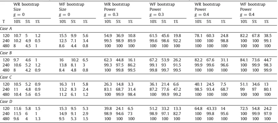
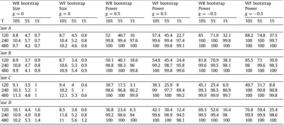
This paper demonstrates the asymptotic validity of methods based on the wild recursive and wild fixed bootstraps for testing hypotheses about discrete parameter change in linear models estimated via Two Stage Least Squares. The framework allows for the errors to exhibit conditional and/or unconditional heteroscedasticity, and for the reduced form to be unstable. Simulation evidence indicates the bootstrap tests yield reliable inferences in the sample sizes often encountered in macroeconomics. If the errors exhibit unconditional heteroscedasticity and/or the reduced form is unstable then the bootstrap methods are particularly attractive because the limiting distributions of the test statistics are not pivotal.
©2019 The Author(s). Published by Elsevier B.V. This is an open access article under the CC
BY-NC-ND license (http://creativecommons.org/licenses/by-nc-nd/4.0/).
1. Introduction
Linear models with endogenous regressors are commonly employed in time series econometric analysis.1 In many
cases, the parameters of these models are assumed constant throughout the sample. However, given the span of many economic time series data sets, this assumption may be questionable and a more appropriate specification may involve parameters that change value during the sample period. Such parameter changes could reflect legislative, institutional or technological changes, shifts in governmental and economic policy, political conflicts, or could be due to large macroeconomic shocks such as the oil shocks experienced over the past decades and the productivity slowdown. It is therefore important to test for parameter – or structural – change. Various tests for structural change have been proposed with one difference between them being in the type of structural change against which the tests are designed to have
∗ Corresponding author.
E-mail addresses: [email protected](O. Boldea),[email protected](A. Cornea-Madeira),[email protected]
(A.R. Hall).
1 For example,Brady(2008) examines consumption smoothing by regressing consumption growth on consumer credit, the latter being endogenous because it depends on liquidity constraints.Zhang et al.(2008),Kleibergen and Mavroeidis(2009),Hall et al.(2012) andKim et al.(2014) investigate the New Keynesian Phillips curve, where inflation is driven by expected inflation and marginal costs, both endogenous since they are correlated with inflation surprises.Bunzel and Enders(2010) andQian and Su(2014) estimate the forward-looking Taylor rule, a model where the Federal fund rate is set based on expected inflation and output, both endogenous as they depend either on forecast errors or on current macroeconomic shocks. All these studies test for structural change in their estimated equations as part of their analysis.
https://doi.org/10.1016/j.jeconom.2019.05.019
power. In this paper, we focus on the scenario in which the potential structural change consists of discrete changes in the parameter values at unknown points in the sample, known as break - (or change-) points. Within this framework, two types of hypotheses tests are of natural interest: tests of no parameter change against an alternative of change at a fixed number of break-points, and tests of whether the parameters change at
ℓ
break-points against an alternative that they change atℓ
+
1 points. These hypotheses tests are of interest in their own right, and also because they can form the basis of a sequential testing strategy for estimating the number of parameter break-points, seeBai and Perron(1998).Hall et al.(2012) propose various statistics for testing these hypotheses in linear models with endogenous regressors based on Two Stage Least Squares (2SLS).2Their tests are the natural extensions of the analogous tests for linear models with exogenous regressors estimated via Ordinary Least Squares (OLS) that are introduced in the seminal paper byBai and Perron(1998). A critical issue in the implementation of these tests in a 2SLS setting is whether or not the reduced form (RF) for the endogenous regressors is stable. If it is then, under certain conditions,Hall et al.’s (2012) test statistics converge in distribution to the same distributions as their OLS counterparts and are pivotal, see Hall et al.(2012) and Perron and Yamamoto(2014). However, if the reduced form itself is unstable and/or there is unconditional heteroskedasticity, then these limiting distributions no longer apply (Hall et al., 2012), and are, in fact, no longer pivotal (Perron and Yamamoto,2014). This is a severe drawback as in most cases of interest the reduced form is likely to be unstable. This problem has been circumvented in two ways.Hall et al.(2012) suggest a testing strategy based on dividing the sample into sub-samples over which the RF is stable but this is inefficient compared to inferences based on the whole sample, and can be infeasible if the sub-samples are small.Perron and Yamamoto (2015) propose using a variant of Hansen’s (2000) fixed regressor bootstrap to calculate the critical values of the test. Their simulation evidence suggests the use of this bootstrap improves the reliability of inferences but they do not establish the asymptotic validity of the method.3
In this paper, we explore the use of bootstrap versions of 2SLS-based tests for parameter change in far greater detail than previous studies. We consider inferences based on two different types of bootstrap versions of the structural change tests, provide formal proofs of their asymptotic validity and report simulation results that demonstrate that the bootstrap tests provide reliable inferences in the finite sample sizes encountered in practice. More specifically, we consider the case where the right-hand side variables of the equation of interest contain endogenous regressors, contemporaneously exogenous variables, lagged values of both and lagged values of the dependent variable. This equation of interest is part of a system of equations that is completed by the reduced form for the endogenous regressors and equations for the contemporaneously exogenous variables. This system of equations is assumed to follow a Structural Vector Autoregressive (SVAR) model in which the parameters of the mean are subject to discrete shifts at a finite number of break-points in the sample. Both the number and location of the break-points are unknown to the researcher. These break-points define regimes over which the parameters are constant, and it is assumed that the implied reduced form VAR is stable within each such regime. The errors of the VAR are assumed to follow a vector martingale difference sequence (m.d.s.) that potentially exhibits both conditional and unconditional heteroskedasticity. Given this error structure, we explore
methods for inference based on the wild bootstrap proposed by Liu (1988) because it has been found to replicate
the conditional and unconditional heteroskedasticity of the errors in other contexts. In particular, we consider two versions of the wild bootstrap: the wild recursive bootstrap (which generates recursively the bootstrap observations) and the wild fixed-regressor bootstrap (which adds the wild bootstrap residuals to the estimated conditional mean, thus keeping all lagged regressors fixed). These bootstraps have been proposed by Gonçalves and Kilian(2004) to test the significance of parameters in autoregressions with (stationary) conditional heteroskedastic errors. Our primary focus is on bootstrap versions of sup-Wald-type statistics to test for structural changes in the parameters of the equation of interest (with endogenous variables) estimated by 2SLS, but our validity arguments also extend straightforwardly to analogous sup-F-type statistics.
While our primary focus is on models where the reduced form for the endogenous regressors is unstable, our results also cover the case where this reduced form is stable. In the latter case, the test statistics have a pivotal limiting distribution under conditions covered by our framework, specialized to errors that are unconditionally homoskedastic. For these situations, the bootstrap methods we propose are expected to provide a superior approximation to finite sample behavior compared to the limiting distribution because the bootstrap, by its nature, incorporates sample information. Thus bootstrap versions of the tests are attractive in this setting as well.
In the case where there are no endogenous regressors in the equation of interest, our framework reduces to a linear model estimated by OLS. For this set-up,Hansen(2000) proposes the wild fixed-design bootstrap to test for structural changes using a sup-F statistic. Very recentlyGeorgiev et al. (2018) consider Hansen’s (2000) bootstrap for versions of sup-F-type tests for parameter variation in predictive regressions with exogenous regressors. BothHansen (2000) andGeorgiev et al.(2018) establish the asymptotic validity of this bootstrap within the settings they consider.4There are some similarities and important differences between our framework (specialized to the no endogenous regressor case) and those inHansen(2000) andGeorgiev et al.(2018). We adopt similar assumptions about the error process to
2 Perron and Yamamoto(2015) propose an alternative approach based on OLS.
3 An alternative approach is to estimate the number and location of the breaks via an information criteria, seeHall et al.(2015). However, this approach has the drawback that inferences can be sensitive to the choice of penalty function.
Georgiev et al.(2018) and like bothHansen(2000) andGeorgiev et al.consider fixed regressor bootstrap tests of a null of constant parameters versus an alternative of parameter change. Important differences include:Georgiev et al.(2018) allow for strongly persistent variables whereas our framework assumes the system is stable within (suitably defined) regimes; our analysis covers tests for additional breaks in the model, the use of the recursive bootstrap and also inferences based on sup-Waldtests. Thus our results for this case complement those ofHansen(2000) andGeorgiev et al.(2018).5
Although the frameworks are different,Hansen(2000),Georgiev et al.(2018) and our own study all find their bootstrap versions of the structural change tests work well in finite samples. Interestingly, Chang and Perron (2018) find that bootstrap-based inferences about the location of breaks have similar advantages in finite samples.6Collectively, our paper and these other recent studies suggest the use of the bootstrap can yield reliable inferences in linear models with multiple break-points in the sample sizes encountered in practice.
An outline of the paper is as follows. Section 2 lays out the model, test statistics and their bootstrap versions. Section3details the assumptions and contains theoretical results establishing the asymptotic validity of the bootstrap methods. Section4contains simulation results that provide evidence on the finite sample performance of the bootstrap tests. Section 5 concludes. Appendix A contains all the tables for Section 4, with additional simulations relegated to
a Supplementary Appendix.7 Appendix B contains the proofs, with some background results relegated to the same
Supplementary Appendix.
Notation: Matrices and vectors are denoted with bold symbols, and scalars are not. Define for a scalarN, the generalized vec operator vects=1:N(As)
=
vect(A1, . . . ,
AN), stacking in order the columns of the matrices As,
s=
1, . . . ,
N. Letdiags=1:N(As)
=
diag(A1, . . . ,
AN) be the matrix that puts the blocksA1, . . . ,
AN on the diagonal. If it is clear over whichsetvectanddiagoperations are taken, then the subscripts
=
1:
Nis dropped on these operators.T denotes the number of time series observations. IfN is the number of breaks in a quantity then T1, . . . ,
TN are the ordered change-points.Also,
τ
N=
(τ
0,
vects=1:N(τ
s)′, τ
N+1) is a partition of the interval[
1,
T]
where each element is divided byT, such that[
Tτ
s] =
Ts,τN, fors=
1, . . . ,
N, andτ
0=
0 andτ
N+1=
1. Define the regimes where parameters are assumed constant asIs,τN
= [
Ts−1+
1,
Ts]
fors=
1, . . . ,
N+
1. Below the breaks in the structural equation are denoted byτ
N=
λ
m, and thosein the reduced form by
τ
N=
π
h, wheremanhare the number of breaks in each equation. A superscript zero on anyquantity refers to the true quantity, which is a fixed number, vector or matrix. For any random vector or matrixZ, denote by
∥
Z∥
the Euclidean norm for vectors, or the Frobenius norm for matrices. Finally,0aand0a×bdenote, respectively, an a×
1 vector and aa×
bmatrix of zeros, and 1Adenotes an indicator function that takes the value one if eventAoccurs.LetmIabe thea
×
aidentity matrix.2. The model and test statistics with their bootstrap versions
This section is divided into three sub-sections. Section2.1outlines the model. Section2.2outlines the hypotheses of interest and the test statistics. Section2.3presents the bootstrap versions of the test statistics.
2.1. The model
Consider the case where the equation of interest takes the form
yt
=
w
′t
1×(p1+q1)β
0(i)
(p1+q1)×1+
ut,
i=
1, . . . ,
m+
1,
t∈
Ii,λ0m,
(1)where
w
t=
vect(xt,
z1,t),z1,t includes the intercept,rt and lagged values ofyt,xt, andrt, andβ
0(i)are the parameters inregimei. The key difference betweenxtandrtis thatxt represents the set of explanatory variables which are correlated
withut, andrt represents the set of explanatory variables that are uncorrelated withut. We therefore refer toxt as the endogenousregressors andrt as thecontemporaneously exogenousregressors.8Eq.(1)can be re-written as:
yt
=
x′tβ
0x,t
+
z′
1,t
β
0z,t
+
ut=
w
′tβ
0 t+
ut,
where
β
0t=
β
0(i)ift∈
Ii,λ0m,
i=
1, . . . ,
m+
1 and similar notation holds forβ
x,t andβ
z,t. For simplicity, we refer to(1)asthe ‘‘structural equation’’ (SE).
5 The wild fixed-regressor bootstrap is also included in the recent simulation study exploring the finite sample properties of inference methods about the location of the break-point in models estimated via OLS reported inChang and Perron(2018).
6 Chang and Perron(2018) report results from a comprehensive simulation study that investigates the finite sample properties of various methods for constructing confidence intervals for the break fractions in linear regression models with exogenous regressors. They consider variants of the intervals based on i.i.d., wild and sieve bootstraps.
7 The Supplementary Appendix is available athttps://sites.google.com/site/otiliaboldea/and in the supplementary material archive of the Journal of Econometrics.
The SE is assumed to be part of a system that is completed by the following equations forxtandrt. The reduced form
(RF) equation for the endogenous regressorsxt is a regression model withhbreaks (h
+
1 regimes), that is:x′
t
1×p1
=
z′t
1×q
∆
0(i)
q×p1
+
v
′t
1×p1,
i=
1, . . . ,
h+
1,
t∈
Ii,π0h
.
(2)The vectorztincludes the constant,rtand lagged values ofyt,xtandrt. It is assumed that the variables inz1,tare a strict
subset of those inzt and therefore we writezt
=
vect(z1,t,
z2,t). Eq.(2)can also be rewritten as:x′t
=
z′t∆
0t+
v
′t,
where
∆
0t=
∆
0(i)ift
∈
Ii,π0h,i
=
1, . . . ,
h+
1. The contemporaneously exogenous variablesrtare assumed to be generatedas follows,
r′t
1×p2=
z′3,tΦ
0(i)+
ζ
′t
1×p2i
=
1, . . . ,
d+
1,
t∈
Ii,ω0d
,
(3)wherez3,t includes the constant and lagged values ofrt,yt andxt.
Eqs.(1),(2)and(3)implyz
˜
t=
vect(yt,
xt,
rt) evolves over time via a SVAR process whose parameters are subject todiscrete shifts at unknown points in the sample. To present the reduced form VAR version of the model, definen
=
dim(z˜
t)and let
τ
Ndenote the partition of the sample such that all three equations have constant parameters within the associatedregimes.9We can then write Eqs.(1),(2)and(3)as:
˜
zt
=
cz˜,s+
p∑
i=1
Ci,sz
˜
t−i+
et,
[
τ
s−1T] +
1≤
t≤ [
τ
sT]
,
s=
1,
2, . . . ,
N+
1,
(4)whereet
=
A−s1ϵ
t,As
=
⎡
⎣
1−
β
0x′,s−
β
0r′,s0p1 Ip1
∆
0′
r,s
0p2 0p2×p1 Ip2
⎤
⎦
,
(5)β
0r′,sdenotes the sub-vector ofβ
0s′that contain the coefficients onrt in(1)(β
0r′,sandβ
0′s are the values of
β
0′r,tand
β
0′t for
[
τ
s−1T] +
1≤
t≤ [
τ
sT]
);∆
0′
r,sdenotes the sub-matrix of
∆
0′s that contains the coefficients onrt in(2)(
∆
0r′,sand∆
0′s
are the values of
∆
0r′,tand∆
0′t for
[
τ
s−1T] +
1≤
t≤ [
τ
sT]
), andϵ
t=
vect(ut,
v
t,
ζ
t). For ease of notation, we assume theorder of the VAR is the same in each regime, but our results easily extend to the case where the order varies by regime.
2.2. Testing parameter variation
As stated in the introduction, this paper focuses on the issue of testing for structural change in the SE. Within the model described above, there are two types of test that are of particular interest. The first tests the null hypothesis of no parameter change against the alternative of a fixed number of parameter changes in the sample that is, a test of
H0
:
m=
0 versusH1:
m=
k. The second tests the null of a fixed number of parameter changes against the alternativethat there is one more, that is, it testsH0
:
m=
ℓ
versusH1:
m=
ℓ
+
1. We consider appropriate test statistics for eachof these scenarios in turn below.
As the tests are based on the Wald principle, calculation of the test statistics here requires 2SLS estimation of the SE underH1. On the first stage, the RF is estimated via least squares methods. If the number and location of the breaks in
the RF are known then this estimation is straightforward. However, in general, neither the number nor the location of the breaks are known and so they must be estimated. For our purposes here, it is important that bothhand
π
0hare consistently estimated and thatπ
ˆ
h, the estimator ofπ
0h, converges sufficiently fast (seeLemma 7inAppendix B). These properties canbe achieved by estimating the RF either as a system or equation by equation, and using a sequential testing strategy to estimateh; see, respectivelyQu and Perron(2007) andBai and Perron(1998). Provided the significance levels of the tests shrink to zero slowly enough,h
ˆ
approaches hwith probability one as the sample sizeT grows;e.g.seeBai and Perron(1998) [Proposition 8]. The same consistency result holds if we estimatehvia the information criteria;e.g.seeHall et al.
(2013). For this reason, in the rest of the theoretical analysis, we treathas known. However, we explore the potential sensitivity of the finite sample performance of the tests for structural change in the SE to the estimation ofh in our simulation study. Let
∆
ˆ
(j)be the estimator of∆
0(j),∆
ˆ
t=
∑
hj=+11∆
ˆ
(j)1t∈ˆIj∗, whereˆ
I∗
j
=
{
[ ˆ
π
j−1T] +
1,
[ ˆ
π
j−1T] +
2, . . . ,
[ ˆ
π
jT]
}
,andx
ˆ
t= ˆ
∆
′
tzt that is,x
ˆ
t is the predicted value forxt from the estimated RF. Case (i): H0:
m=
0versus H1:
m=
k9 For example, suppose m = 1, h = 2 and d = 1 withλ0
m = [0,0.5,1]
′, π0
h = [0,0.3,0.5,1]
′ and ω0
d = [0,0.7,1]
′, then N = 3 and
UnderH1, the second stage estimation involves estimation via OLS of the model,
yt
= ˆ
w
′tβ
(i)+
error,
i=
1, . . . ,
k+
1,
t∈
Ii,λk,
(6)for all possiblek-partitions
λ
k. Letβ
ˆ
(i) denote the OLS estimator ofβ
(i)in(6),β
ˆ
λk≡
vecti=1:k+1(β
ˆ
(i))=
vecti=1:k+1(β
ˆ
i,λk)denote the OLS estimator ofvecti=1:k+1(
β
(i))≡
vecti=1:k+1(β
i,λk) in(6)(that is,β
ˆ
λkis the OLS estimator ofvecti=1:k+1(β
(i))based on partition
λ
k). To present the sup-Waldtest, we defineRk= ˜
Rk⊗
IpwhereR˜
kis thek×
(k+
1) matrix whose(i
,
j)thelement,R˜
k(i,
j), is given by:R˜
k(i,
i)=
1,R˜
k(i,
i+
1)= −
1,R˜
k(i,
j)=
0 fori=
1,
2, . . . ,
k, andj̸=
i,j̸=
i+
1. Alsolet
Λ
ϵ,k= {
λ
k: |
λ
i+1−
λ
i|≥
ϵ, λ
1≥
ϵ, λ
k≤
1−
ϵ
}
. With this notation, the test statistic is:sup -WaldT
=
supλk∈Λϵ,k
WaldTλk
,
(7)WaldTλk
=
Tβ
ˆ
′
λkR
′
k
(
RkV
ˆ
λkR′
k
)
−1Rk
β
ˆ
λk,
(8)where:
ˆ
Vλk
=
diagi=1:k+1(Vˆ
(i)),
Vˆ
(i)= ˆ
Q−1 (i) M
ˆ
(i)Qˆ
−1
(i)
,
Qˆ
(i)=
T−1∑
t∈Ii,λk
ˆ
w
tw
ˆ
′
t
,
(9)ˆ
M(i) p
→
limT→∞Var
⎛
⎝
T−1/2∑
t∈Ii,λkΥ
0t′zt(
ut
+
v
′tβ
0x
)
⎞
⎠
,
(10)β
0xis the true value ofβ
0x,(i)fori=
1,
2, . . . ,
m+
1 underH0, andΥ
0t=
(∆
0t
,
Π
) andΠ
′
=
(
Iq1
,
0q1×(q−q1))
.
As mentioned in the introduction, our framework assumes the errors are a m.d.s. that potentially exhibits heteroskedas-ticity, and so the natural choice ofM
ˆ
(i) is the Eicker–White estimator, seeEicker(1967) andWhite(1980). This can beconstructed using the estimator of
β
x,(i)in(6)under eitherH0orH1, whereβ
x,(i)are the elements ofβ
(i) containing thecoefficients on x
ˆ
t. For the purposes of the theory presented below, it does not matter which is used because the nullhypothesis is assumed to be true. However, the power properties may be sensitive to this choice. In our simulation study reported below, we use the Eicker–White estimator based on
β
ˆ
x,(i), the estimator ofβ
x,(i)underH1, that is,ˆ
M(i)
=
ˆ
EW[
ˆ
Υ
t′zt(uˆ
t+ ˆ
v
′tβ
ˆ
x,(i));
Ii,λk]
,
whereu
ˆ
t=
yt−
w
′tβ
ˆ
(i)fort∈
Ii,λk,v
ˆ
t=
xt− ˆ
∆
′
tzt,
Υ
ˆ
t= [ ˆ
∆
t,
Π
]
,∆
ˆ
tis defined before(6),β
ˆ
x,(i)are the firstp1elementsof
β
ˆ
(i), and for any vectorat andI⊆ {
1,
2, . . . ,
T}
,EWˆ
[at;
I]=
T−1∑
t∈Iata′t. Case (ii): H0:
m=
ℓ
versus H1:
m=
ℓ
+
1Following the same approach used byBai and Perron(1998) for OLS based inferences, suitable tests statistics can be constructed as follows. The model with
ℓ
breaks is estimated via a global minimization of the sum of squared residuals associated with the second stage of the 2SLS estimation of the SE. For each of theℓ
+
1 regimes of this estimated model, the sup-Waldstatistic for testing no breaks versus one break is calculated. Inference aboutH0:
m=
ℓ
versusH1:
m=
ℓ
+
1is based on the largest of these
ℓ
+
1 sup -Waldstatistics.More formally, let the estimated SE break fractions for the
ℓ
-break model beλ
ˆ
ℓ and the associated break pointsbe denoted
{ ˆ
Ti}
ℓi=1 where Tˆ
i= [
Tλ
ˆ
i]
. Letˆ
Ii=
Ii,λˆℓ, the set of observations in the ith regime of theℓ
-break modeland partition this set as
ˆ
Ii= ˆ
Ii(1)(ϖ
i)∪ ˆ
Ii(2)(ϖ
i) whereˆ
Ii(1)(ϖ
i)= {
t: [ ˆ
λ
i−1T] +
1,
[ ˆ
λ
i−1T] +
2, . . . ,
[
ϖ
iT]}
andˆ
Ii(2)(
ϖ
i)= {
t: [
ϖ
iT] +
1,
[
ϖ
iT] +
2, . . . ,
[ ˆ
λ
iT]}
. Consider the estimation of the modelyt
= ˆ
w
′tβ
(j)+
error,
j=
1,
2,
t∈ ˆ
I (j)i (
ϖ
i),
(11)for all possible choices of
ϖ
i (where for notational brevity we suppress the dependence ofβ
(j) on i). Letβ
ˆ
(ϖ
i)=
vect
(
β
ˆ
(1)(ϖ
i),
β
ˆ
(2)(ϖ
i))
be the OLS estimators ofvect(
β
(1),
β
(2)) from(11). Also letNi(λ
ˆ
ℓ)= [ ˆ
λ
i−1+
ϵ,
λ
ˆ
i−
ϵ
]
. The sup -Waldstatistic for testingH0
:
m=
ℓ
versusH1:
m=
ℓ
+
1 is given bysup -WaldT(
ℓ
+
1|
ℓ
)=
maxi=1,2,...,ℓ+1
{
sup
ϖi∈Ni(λˆℓ)
T
β
ˆ
(ϖ
i)′R′1[
R1Vˆ
(ϖ
i)R′1]
−1R 1
β
ˆ
(ϖ
i)}
(12)
where10
ˆ
V(
ϖ
i)=
diag(
ˆ
V1(
ϖ
i),
Vˆ
2(ϖ
i))
,
Vˆ
j(ϖ
i)= { ˆ
Qj(ϖ
i)}
−1Mˆ
j(ϖ
i){ ˆ
Qj(ϖ
i)}
−1,
ˆ
Qj(
ϖ
i)=
T−1∑
t∈ˆIi(j)
ˆ
w
tw
ˆ
′t,
Mˆ
j(ϖ
i)=
EWˆ
[
ˆ
Υ
′tzt(uˆ
t+ ˆ
v
′tβ
ˆ
x,(j)(ϖ
i)); ˆ
Ii(j)(ϖ
i)]
,
whereu
ˆ
t=
yt−
w
′tβ
ˆ
(j)(ϖ
i) fort∈ ˆ
Ii(j)(ϖ
i),j=
1,
2,v
ˆ
t=
xt− ˆ
∆
′
tzt,
Υ
ˆ
t= [ ˆ
∆
t,
Π
]
,∆
ˆ
tis defined before(6), andβ
ˆ
x,(j)(ϖ
i)are the firstp1elements of
β
ˆ
(j)(ϖ
i).2.3. Bootstrap versions of the test statistics
In this section, we introduce the bootstrap analogues of the test statistics presented in the previous section. As noted above, our framework assumes the error vector
ϵ
t to be a m.d.s that potentially exhibits conditional and unconditionalheteroskedasticity, and so we use the wild bootstrap proposed byLiu(1988) because it has been found to replicate the conditional and unconditional heteroskedasticity of the errors in other contexts.11We consider both the wild recursive (WR) bootstrap and the wild fixed regressor (WF) bootstrap. These procedures differ in their treatment of the right-hand side variables in the bootstrap samples as described below.
Generation of the bootstrap samples:
Let z
˜
bt=
vect(ybt
,
xbt,
rt) where ybt and xbt denote the bootstrap values of yt and xt. Note that because rt iscontemporaneously exogenous its sample value is used in the bootstrap samples. In all cases below, the bootstrap residuals are obtained asub
t
= ˆ
utν
t andv
bt= ˆ
v
tν
t, whereuˆ
t andv
ˆ
t are the (non-centered) residuals under the null hypothesis andν
t is a random variable that is discussed further in Section3(Assumption 10).For the WR bootstrap,
{
ybt′}
and{
xbt′}
are generated recursively as follows:xtb′
=
zbt′∆
ˆ
t+
v
bt′,
(13)ytb
=
xbt′β
ˆ
x,t+
z1b′,tβ
ˆ
z,t+
ubt,
(14)where the vectorzb
t contains a constant,rt and lags ofybt,xbt andrt;
β
ˆ
x,t andβ
ˆ
z,t are the sample estimates ofβ
0x,t and
β
0z,t underH0of the test in question.For the WF bootstrap,ztis kept fixed and, followingGonçalves and Kilian(2004), the bootstrap samples are generated
as follows:
xbt′
=
z′t∆
ˆ
t+
v
bt′,
(15)yb t
=
xb′
t
β
ˆ
x,t+
z′
1,t
β
ˆ
z,t+
ubt,
(16)where again
β
ˆ
x,tandβ
ˆ
z,t are the sample estimates ofβ
0x,t andβ
0z,t underH0of the test in question.Case (i): H0
:
m=
0vs H1:
m=
kFirst consider the WR bootstrap. 2SLS estimation is implemented in the bootstrap samples as follows. On the first stage, the following model is estimated via OLS
xbt′
=
zbt′∆
j+
error,
t∈ ˆ
Ij∗,
j=
1,
2, . . . ,
h+
1,
to obtain
∆
ˆ
bj=
{∑
t∈ˆIj∗zbtzbt′
}
−1∑
t∈ˆIj∗zbtxbt′. Define
∆
ˆ
b t=
∑
hˆ+1 j=1 1t∈ˆI∗j∆
ˆ
b j,x
ˆ
b′
t
=
zbt′∆
ˆ
b t, andw
ˆ
b
t
=
vect(xˆ
bt
,
zb1,t). For a given k-partitionλ
k, the second stage of the 2SLS in the bootstrap samples involves OLS estimation ofybt
= ˆ
w
bt′β
(i)+
error,
i=
1, . . . ,
k+
1,
t∈
Ii,λk,
(17)and let
β
ˆ
bλk≡
vecti=1:k+1(β
ˆ
b(i))
=
vecti=1:k+1(β
ˆ
bi,λk) be the resulting OLS estimator ofvecti=1:k+1(
β
(i))≡
vecti=1:k+1(β
i,λk)based on partition
λ
k. The WR bootstrap version of the sup-WaldTstatistic is:sup -WaldbT
=
supλk∈Λϵ,k
WaldbTλ
k
,
(18)Waldb
Tλk
=
Tβ
ˆ
b′λkR
′
k
(
RkV
ˆ
b λkR′
k
)
−1Rk
β
ˆ
bλk
,
(19)where:
ˆ
Vbλ
k
=
diagi=1:k+1(ˆ
Vb(i))
,
Vˆ
b(i)=
(Qˆ
b(i))−1Mˆ
b(i)(Qˆ
b(i))−1,
Qˆ
b(i)=
T−1∑
t∈Ii,λkˆ
w
btw
ˆ
bt′,
(20)ˆ
Mb(i)
=
ˆ
EW[
Υ
ˆ
bt′zbt(
uˆ
bt+ ˆ
v
tb′β
ˆ
bx,(i))
;
Ii,λk]
,
(21)whereu
ˆ
bt
=
ybt−
w
bt′β
ˆ
b(i) fort
∈
Ii,λk,v
ˆ
bt
=
xbt− ˆ
∆
b′tzbt,
Υ
ˆ
b t=
(∆
ˆ
b t
,
Π
),∆
ˆ
b
t is defined before(17),
w
bt=
vect(xbt,
zb1,t), andˆ
β
bx,(i)are the firstp1elements ofβ
ˆ
b (i).Now consider the WF bootstrap, for whichyb
t andxbt are generated via(15)–(16). The first stage of the 2SLS involves
LS estimation of
xbt
=
z′t∆
j+
error,
t∈ ˆ
Ij∗,
j=
1,
2, . . . ,
h+
1,
to obtain
∆
ˆ
bj=
{∑
t∈ˆI∗j ztz′t
}
−1∑
t∈ˆI∗j ztxbt′. Now re-define
∆
ˆ
b t=
∑
hˆ+1 j=11t∈ˆIj∗∆
ˆ
b j,x
ˆ
b′
t
=
z′t∆
ˆ
b t, andw
ˆ
b
t
=
vect(xˆ
b t,
z1,t).For a givenk-partitions
λ
k, the second stage of the 2SLS in the bootstrap samples involves OLS estimation of(17)and letˆ
β
bλk=
vecti=1:k+1(β
ˆ
b(i)) be the resulting OLS estimator ofvecti=1:k+1(
β
(i)) based on partitionλ
k. The WF bootstrap sup -Waldstatistic is defined as in(18)withWaldbTλ
kdefined as in(19)only with
w
ˆ
b t and∆
ˆ
b
t redefined in the way described in this
paragraph, and M
ˆ
b(i) in (21)replaced byMˆ
b(i)=
ˆ
EW[
Υ
ˆ
bt′zt(uˆ
bt+ ˆ
v
b′t
β
ˆ
bx,(i))
;
Ii,λk]
, whereu
ˆ
bt
=
ybt−
w
b′
t
β
ˆ
b(i) for t
∈
Ii,λk,ˆ
v
bt=
xb t− ˆ
∆
b′
tzt,
Υ
ˆ
b t=
(∆
ˆ
b
t
,
Π
),w
bt=
vect(xbt,
z1,t), andβ
ˆ
bx,(i) are the firstp1elements of
β
ˆ
b (i).Case (ii): H0
:
m=
ℓ
versus H1:
m=
ℓ
+
1For each bootstrap the first stage of the 2SLS estimation and the construction of
w
ˆ
t is the same as described under Case (i)above. Letˆ
Ii(j)be defined as in the discussion ofCase (ii)in Section2.2, and considerybt
= ˆ
w
bt′β
(j)+
error,
j=
1,
2 t∈ ˆ
Ii(j),
(22)for all possible choices of
ϖ
i(where, once again, we suppress the dependence ofβ
(j)oni). Letβ
ˆ
b(
ϖ
i)=
vect(
ˆ
β
b(1)(ϖ
i),
ˆ
β
b(2)(ϖ
i))
be the OLS estimators ofvect(
β
(1),
β
(2)) from(22). The bootstrap version of sup -WaldT(ℓ
+
1|
ℓ
) is given bysup -WaldbT(
ℓ
+
1|
ℓ
)=
maxi=1,2,...,ℓ+1
{
sup
ϖi∈N(λˆℓ)
T
β
ˆ
b(ϖ
i)′R′1[
R1Vˆ
b(
ϖ
i)R′1]
−1
R1
β
ˆ
b(
ϖ
i)}
(23)
where
ˆ
Vb(
ϖ
i)=
diag(
ˆ
Vb1(
ϖ
i),
Vˆ
b 2(ϖ
i))
,
Vˆ
bj(ϖ
i)= { ˆ
Q bj(
ϖ
i)}
−1Mˆ
b j(ϖ
i){ ˆ
Qb j(
ϖ
i)}
−1,
ˆ
Qbj(
ϖ
i)=
T−1∑
t∈ˆIi(j)
ˆ
w
btw
ˆ
bt′,
andM
ˆ
bj(ϖ
i)=
ˆ
EW[
ˆ
Υ
bt′zbt(uˆ
bt+ ˆ
v
b′t
β
ˆ
bx,(j)(
ϖ
i)); ˆ
I (j) i (ϖ
i)]
for the WR bootstrap, whereu
ˆ
bt
=
ybt−
w
bt′β
ˆ
b(j)(
ϖ
i) fort∈ ˆ
I (j) i (ϖ
i),ˆ
v
bt=
xb t− ˆ
∆
b′
tzbt,
Υ
ˆ
b t=
(∆
ˆ
b t
,
Π
),∆
ˆ
b
t is defined before(17),
w
bt=
vect(xbt,
zb1,t), andβ
ˆ
bx,(j)(
ϖ
i) are the firstp1elementsof
β
ˆ
b(j)(ϖ
i); andMˆ
bj(
ϖ
i)=
ˆ
EW[
ˆ
Υ
bt′zt(uˆ
bt+ ˆ
v
b′t
β
ˆ
bx,(j)(
ϖ
i)); ˆ
Ii(j)(ϖ
i)]
for the WF bootstrap, whereu
ˆ
bt
=
ybt−
w
bt′β
ˆ
b (j)(ϖ
i)for t
∈ ˆ
Ii(j)(ϖ
i),v
ˆ
bt=
xbt− ˆ
∆
b′tzt,
Υ
ˆ
b t=
(∆
ˆ
b t
,
Π
),∆
ˆ
b
t is defined in the last paragraph ofCase (i) in this section,
w
bt
=
vect(xbt,
z1,t), andβ
ˆ
bx,(j)(
ϖ
i) are the firstp1elements ofβ
ˆ
b (j)(ϖ
i).3. The asymptotic validity of the bootstrap tests
In this section, we establish the asymptotic validity of the bootstrap versions of the test statistics described above. To this end we impose the following conditions.
Assumption 1. Ifm
>
0,T0i
= [
Tλ
0i]
, where 0< λ
01<
· · ·
< λ
0m<
1.Assumption 2. Ifm
>
0,β
0(i+1)−
β
0(i)is a non-zero vector of constants fori=
1, . . . ,
m.Assumption 3. Ifh
>
0, thenT∗i
= [
Tπ
i0]
, where 0< π
10<
· · ·
< π
h0<
1.Assumption 4. Ifh
>
0,∆
0(j+1)−
∆
0(j)is a non-zero matrix of constants forj
=
1, . . . ,
h.Assumption 5. Ifk
>
0, then 0< ω
01<
· · ·
< ω
0k<
1 andΦ
0(i+1)−
Φ
0(i)is a non-zero matrix of constants fori
=
1, . . . ,
k.Assumption 6. The first and second stage estimations in 2SLS are over respectively all partitions of
π
andλ
such thatAssumption 7.(i)p
<
∞
; (ii)⏐
⏐
In−
C1,sa−
C2,sa2−
. . .
−
Cp,sap⏐
⏐
̸=
0, for alls=
1, . . . ,
N+
1, and all|
a| ≤
1.Assumption 8. rk
(
Υ
0t)
=
p1+
q1.Assumption 9. The innovations can be written as
ϵ
t=
SDtlt, where:(i)Sis an
×
nlower triangular non-stochastic matrix with real-valued diagonal elementssii=
1 and elements belowthe diagonal equal tosij(which are also zero fori
>
p1+1,
j<
p1+1), such thatSS′is positive definite;Dt=
diagi=1:n(dit),a non-stochastic matrix wheredit
=
di(t/
T): [
0,
1] →
Dn[
0,
1]
, the space of cadlag strictly positive real-valued functionsequipped with the Skorokhod topology;
(ii)lt
=
vect(lu,t,
lv,t,
lζ,t) is an×
1 vector m.d.s. w.r.t toFt= {
lt,
lt−1, . . .
}
to which it is adapted, with conditionalcovariance matrix
Σ
t|t−1=
E(ltl′t|
Ft−1)=
diag(
Σ
(1)t|t−1,
Σ
(2) t|t−1)
and unconditional variance E(ltl′t)
=
In.(iii) suptE
∥
lt∥
4+δ<
∞
for someδ >
0; E∥
ξ
0∥
4<
∞
, whereξ
0=
vect(z˜
0,
z˜
−1, . . . ,
z˜
−p+1).(iv) E
(
(ltl′t)⊗
lt−i)
=
ρ
ifor alli≥
0, with supi≥0∥
ρ
i∥
<
∞
.(v) E
(
(ltl′t)⊗
(lt−il′t−j))
=
ρ
i,j, for alli,
j≥
0 with supi,j≥0∥
ρ
i,j∥
<
∞
.Assumption 9′. Letn
t
=
vect(lu,t,
lv,t). Then:(i)Assumption 9(iv) holds with E
[
(ntn′t)⊗
nt−i] =
0(p1+1)2×(p1+1) for alli≥
1.(ii)Assumption 9(v) holds with E
[
(ntn′t)⊗
(nt−in′t−j)] =
0(p1+1)2×(p1+1)2 for alli,
j≥
1 andi̸=
j.(iii)Assumption 9(v) holds with E
[
(ntn′t)⊗
(nt−il′ζ,t−j)] =
0(p1+1)2×(p1+1)p2 for alli≥
1 andj≥
0.(iv) suptE
∥
lt∥
8<
∞
.Assumption 10.(i)
ν
t i.i.d.∼
(0,
1) independent of the original data generated by(1),(2)and(3); (ii) Eb|
ν
t|
4+δ∗
= ¯
c<
∞
, for someδ
∗>
0, for allt, where Ebdenotes the expectation under the bootstrap measure.Before presenting our main theoretical results, we discuss certain aspects of the assumptions.
Remark 1. Assumptions 1–5indicate that the breaks are ‘‘fixed’’ in the sense that the size of the associated shifts in the parameters between regimes is constant and does not change with the sample size.
Remark 2. It follows fromAssumption 7thatz
˜
t follows a finite order VAR in(4)that is stable within each regime.Remark 3. Assumption 8is the identification condition for estimation of the structural equation parameters; seeHall et al.(2012) for further discussion.
Remark 4. FromAssumption 9it follows that
ϵ
t is a vector m.d.s. relative toFt−1 with time varying conditional andunconditional variance given by E(
ϵ
tϵ
′t|F
t−1)=
SDtΣ
t|t−1D′tS′and E(
ϵ
t
ϵ
′t)=
SDtD′tS′respectively. The m.d.s. property
implies that all the dynamic structure in the SE for yt and RF for xt is accounted for by the variables in z1,t and
zt respectively. As noted by Boswijk et al. (2016) and Georgiev et al. (2018), Assumption 9 allows for
ϵ
t to exhibitconditional and unconditional heteroskedasticity of unknown and general form that can include single or multiple variance
shifts, variances that follow a broken trend or follow a smooth transition model. WhenDt
=
D, the unconditionalvariance is constant but we may have conditional heteroskedasticity. When
Σ
t|t−1=
In, the unconditional variancemay still be time-varying. Note that Assumption 9(i)–(ii) imply that xt is endogenous and rt is contemporaneously
exogenous in the SE.Assumption 9(iii) is a moment condition aboutlt (similar to Assumption A(iv) inGonçalves and Kilian(2004) and Assumption 2(iv) inBoswijk et al.(2016)) and a moment condition on the initial values of the VAR in
(4).Assumption 9(iv) allows for leverage effects (the correlation between the conditional variance andlt−i is nonzero,
wheni
≥
1).Assumption 9(v) allows for (asymmetric) volatility clustering (the conditional variance is correlated with cross-productslt−ilt−j, fori,
j≥
1).12Remark 5. Assumption 9′is only imposed in the case of the WR bootstrap.Assumption 9′(i)–(iii) is needed because the WR bootstrap sets to zero certain covariance terms in the distribution of the bootstrapped parameter estimates given the data. This happens because these moments depend on products of bootstrap errors at different lags and these terms have zero expectation under the bootstrap measure due to the fact that
ν
tis mean zero and i.i.d.Assumption 9′(i) is a restrictionon the leverage effects andAssumption 9′(ii) is a restriction of the asymmetric effects allowed in volatility clustering. Note thatAssumption 9′(i) is only needed when we have an intercept in(4).Assumption 9′(iii) arises because the WR design bootstraps the lags ofytandxt in(4), but it does not bootstraprt and its lags. Therefore, certain fourth cross-moments
involving both types of quantities are set to zero by the WR bootstrap, leading to the restriction on clustering effects in
Assumption 9′(iii) (wherei
=
jis imposed for replicating certain variances, andi̸=
jis imposed for replicating certaincovariances in the asymptotic distribution of the parameter estimates).Assumption 9′(iv) is needed in order to verify one of the conditions of the CLT for m.d.s., by ensuring the convergence of the WR bootstrap variance to the correct limiting variance.Assumption 9′(iv) is similar to Assumption A′(vi′) inGonçalves and Kilian(2004) and Assumption 2′inBoswijk et al.(2016). However,Assumption 9′(iv) can be replaced withAssumption 9(iii) if
ν
t (inAssumption 10) used in the WR
bootstrap follows the Rademacher two point distribution suggested inLiu(1988).13
Remark 6. There are several choices for the distribution of
ν
t, the random variable used in construction of thebootstrap errors: Gonçalves and Kilian(2004) use the standard normal distribution, whileMammen(1993) suggested an asymmetric two-point distribution andLiu (1988) suggested the Rademacher two-point distribution. In this paper, we report simulation results for Liu’s (1988) two-point distribution, which we found performed the best compared to the other distributions in simulations not reported here. This conclusion is similar to Davidson and Flachaire (2008) andDavidson and MacKinnon(2010).
The following theorems establish the asymptotic validity of the bootstrap versions of thesup-Waldtests.
Theorem 1. If the WF bootstrap is used letAssumptions1–10hold and if the WR bootstrap is used letAssumptions1–10and 9′hold. If yt,xt andrt are generated by(1),(2)and(3)and m
=
0then it follows thatsup
c∈R
⏐
⏐
Pb(
sup-WaldbT≤
c)
−
P(sup-WaldT≤
c)⏐
⏐
p→
0as T
→ ∞
, where Pbdenotes the probability measure induced by the bootstrap.Theorem 2. If the WF bootstrap is used letAssumptions1–10hold and if the WR bootstrap is used letAssumptions1–10and 9′hold. If y
t,xt andrt are generated by(1),(2)and(3)and m
=
ℓ
then it follows that:sup
c∈R
⏐
⏐
Pb(
sup-WaldbT(ℓ
+
1|
ℓ
)≤
c)
−
P(sup-WaldT(ℓ
+
1|
ℓ
)≤
c)⏐
⏐
p→
0as T
→ ∞
, where Pbdenotes the probability measure induced by the bootstrap.Remark 7. The proof rests on showing the sample and bootstrap statistics have the same limiting distribution. Although this distribution is known to be non-pivotal if the RF is unstable (seePerron and Yamamoto, 2014), to our knowledge this distribution has not previously been presented in the literature. A formal characterization of this distribution is provided in the Supplementary Appendix.
Remark 8. Theorem 1–2 cover the case where the reduced form is stable and the errors are unconditionally
homoskedastic. In this case, the sup-Waldtests are asymptotically pivotal and so the bootstrap is expected to provide a superior approximation to finite sample behavior compared to the limiting distribution because the bootstrap, by its nature, incorporates sample information. However, a formal proof is left to future research.
Remark 9. Hall et al.(2012) also propose testing the hypotheses described above using sup-F tests. WhileF-tests are designed for use in regression models with homoskedastic errors,14wild bootstrap versions of the tests can be used as a basis for inference when the errors exhibit heteroskedasticity. In the Supplementary Appendix, we present WR bootstrap and WF bootstrap versions of appropriate sup-F statistics for testing bothH0
:
m=
0 versusH1:
m=
kandH0:
m=
ℓ
versusH1
:
m=
ℓ
+
1, and show that these bootstrap versions of the sup-Ftests are asymptotically valid under the sameconditions as their sup-Waldcounterparts. Simulation evidence indicated no systematic difference in the finite sample behavior of the sup-Waldand sup-Ftests for a given null and bootstrap method, and so further details about this approach are relegated to the Supplementary Appendix.
Remark 10. In the special case where there are no endogenous regressors in the equation of interest then our framework reduces to one in which a linear regression model is estimated via OLS. For this set-up, the asymptotic validity of wild fixed bootstrap versions of sup-F test for parameter variation (our Case(i) above) has been established under different sets of conditions byHansen(2000) andGeorgiev et al.(2018).Hansen(2000) considers the case where the marginal distribution of the exogenous regressors changes during the sample.Georgiev et al.(2018) considerHansen’s (2000) bootstrap in the context of predictive regressions with strongly persistent exogenous regressors. Our results complement these earlier studies because we provide results for the wild recursive bootstrap and a theoretical justification for tests of
ℓ
breaks againstℓ
+
1 based on bootstrap methods.13 See the proof ofLemma 10.