Value-Gradient Learning

(1)

City, University of London Institutional Repository

Citation

:

Fairbank, M. (2014). Value-Gradient Learning. (Unpublished Doctoral thesis, City University London)

This is the unspecified version of the paper.

This version of the publication may differ from the final published

version.

Permanent repository link:

http://openaccess.city.ac.uk/3438/

Link to published version

:

Copyright and reuse:

City Research Online aims to make research

outputs of City, University of London available to a wider audience.

Copyright and Moral Rights remain with the author(s) and/or copyright

holders. URLs from City Research Online may be freely distributed and

linked to.

City Research Online: http://openaccess.city.ac.uk/ [email protected]

(2)

Value-Gradient Learning

Michael Fairbank

A thesis submitted for the degree of

PhilosophiæDoctor (PhD)

School of Informatics Department of Computer Science

(3)

(4)

(5)

(6)

List of Figures

1.1 Relationship of VGL(λ) to other ADPRL algorithms. . . 16

2.1 State-Space View of Vertical-Lander Trajectories . . . 47

2.2 Results for Using a Stochastic Policy to Solve the Vertical-Lander Prob-lem by TD(λ) . . . 50

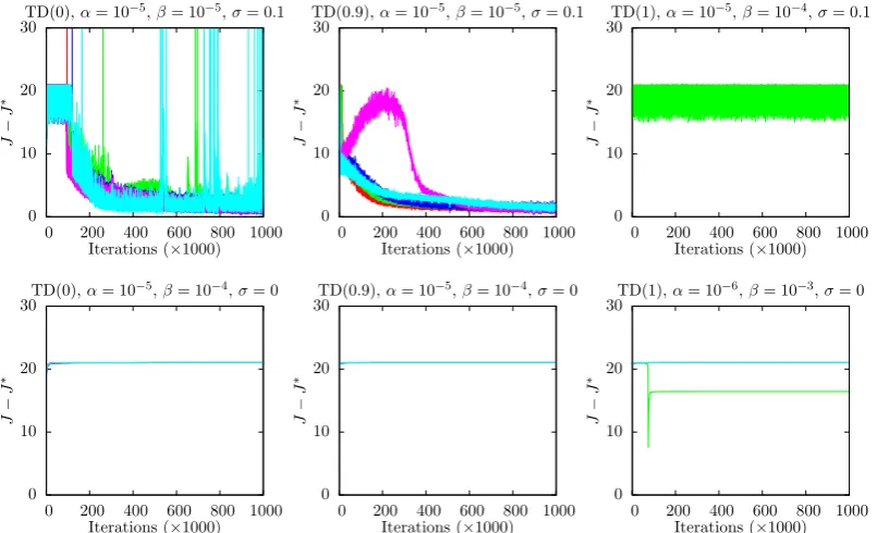
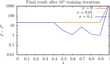
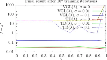
2.3 Results of TD(λ) Under Various λ and Noise-Levels σ, for Solving the Vertical-Lander Problem, from a Fixed Trajectory Start Point . . . 51

2.4 Results for Using Exploring Starts to Solve the Vertical-Lander Problem by TD(λ) . . . 52

3.1 The Motivation of Automatic Local Value Exploration for VGL in the Vertical-Lander Problem. . . 57

3.2 The Portion of Value-Function Surface Learned by VGL Compared to that Learned by VL . . . 59

3.3 Scalar Critic . . . 66

3.4 Vector Critic . . . 66

3.5 A Non-Zero Curl Field Allowed by a Vector Critic . . . 66

3.6 Trajectory Optimality under a Greedy Policy, for Value-Gradient Learning 78 3.7 Results for Using a Stochastic Policy to Solve the Vertical-Lander Prob-lem by VGL(λ) . . . 79

3.8 Results of VGL(λ) Under Variousλand Noise-Levelsσ, for Solving the Vertical-Lander Problem, from a Fixed Trajectory Start Point . . . 80

(15)

3.10 Algorithm Performances for the Quadratic-Optimisation Problem of

Sec-tion 3.7 . . . 83

4.1 Value-Function Surface and Roller-Coaster Shaped Trajectory Profile. . 91

4.2 Roller-Coasters With and Without Track Shear . . . 92

5.1 Greedy-Policy Versus Actor-Critic Performance on the Fixed-Duration

Vertical-Lander Problem . . . 119

5.2 VGL(0) and VGL(1) performance on the Fixed-Duration Vertical-Lander,

with a Greedy Policy, using RPROP. . . 120

5.3 VGLΩ(1), with a Greedy Policy, using RPROP, on the Fixed-Duration

Vertical-Lander Problem . . . 121

5.4 Cart-Pole Benchmark Problem . . . 122

5.5 Cart-Pole Solutions by VGL(0), VGL(1), VGLΩ(1) and BPTT, with a

Greedy Policy . . . 124

6.1 Application of BPTT for Control Problems. . . 131

7.1 Trajectory Optimality Occurs when the Value-Gradients are Learned,

under a Greedy Policy . . . 145

8.1 The Equivalence of VGLΩ(1) to BPTT, and the Implied Convergence

Proof. . . 159

9.1 Divergence for VGL(1) and VGL(0) under a Greedy Policy; Convergence

for VGLΩ(1). . . 179

9.2 Divergence for TD(0) under a Greedy Policy . . . 181

9.3 Divergence for TD(1) under a Greedy Policy . . . 181

9.4 The Performance of TD(0) and TD(1) in the Divergence Problem in the

Absence of Stochastic Value Exploration . . . 182

10.1 A Trajectory Reaching a Terminal State, without Clipping. . . 187

10.2 An Example of the Problems that Can Occur when Clipping is Not Used188

10.3 A Pathological Example: Local gradient is Opposite to Global Gradient. 189

10.4 The Final State Transition of a Trajectory Crossing the Tangent Plane

(16)

LIST OF FIGURES

10.5 The Discontinuous Change in Derivatives of the Model Functionf(~x, ~u, ~e) at a Terminal Boundary . . . 195

10.6 Vertical-Lander Solutions by BPTT, VGL(0), VGL(1) and HDP using

∆τ = 1. . . 201

10.7 Vertical Lander with ∆τ = 0.01. . . 201

10.8 Cart-Pole Solutions by BPTT, VGL(0), VGL(1) and HDP . . . 204

11.1 An Example Neural-Network Architecture Obtainable by Alg. 11.1 . . . 211

11.2 Outputs from a Sample of Five Neural Networks Created to Learn the

Shape of a Sinusoidal Wave. . . 217

11.3 Results for Using a Scalar Critic and a Vector Critic to Solve the Problem

(17)

(18)

List of Tables

1.1 Common Notational Differences (and Similarities) between ADP and RL 23

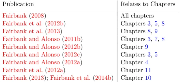
1.2 Publications Resulting from this Thesis . . . 25

2.1 Network Architectures used for Vertical-Lander Experiments . . . 49

2.2 Start-State Coordinates used for Exploring-Starts Vertical-Lander Ex-periment . . . 51

5.1 Some Common ADPRL Action-Network Weight Updates . . . 102

5.2 Common Choices forg(x) in the Closed-Form Greedy Policy . . . 107

6.1 Common Policy-Gradient Action-Network Weight Updates . . . 130

10.1 Terminal Boundary Planes used in Vertical-Lander Experiment. . . 200

10.2 Terminal Boundary Planes used in Cart-Pole Experiment. . . 202

(19)

(20)

List of Algorithms

1.1 Trajectory Unroll and Total-Cost Calculation in the ADPRL problem. . 12

2.1 Actor-Critic, On-Line Implementation of TD(0)/HDP Algorithms, in-cluding an ADP action-network weight update. . . 31

2.2 Actor Critic, On-Line Implementation of TD(λ) using Eligibility Traces, including an Action-Network Weight Update from ADP. . . 32

3.1 Actor-Critic, On-Line Implementation of DHP algorithm. . . 64

3.2 VGL(λ). Actor-Critic, Batch-Mode Implementation for Episodic Envi-ronments. . . 72

3.3 VGL(λ). Actor-Critic, On-Line Implementation. . . 73

5.1 VGL(λ) with a Sigmoidal Continuous-Time Greedy Policy. Batch-Mode Implementation for Episodic Environments. . . 112

5.2 VGL(λ) with a Sigmoidal Discrete-Time Greedy Policy. Batch-Mode Implementation for Episodic Environments. . . 114

6.1 Backpropagation Through Time for Control. . . 133

10.1 Unrolling a Trajectory with Clipping. . . 193

10.2 Backpropagation Through Time for Control, with Clipping. . . 197

10.3 VGL(λ), with Clipping; Actor-Critic, Batch-Mode Implementation. . . . 198

11.1 Feed-Forward Dynamics of a Neural Network, Followed by First-Order Error Backpropagation to Calculate ∂y_∂~_x. . . 211

(21)

(22)

Acknowledgements

I would like to thank my family for their support throughout the duration

of this research, in particular to my wife, parents, brother and the family

in Olkusz. I would also like to express my gratitude to my supervisor

Eduardo Alonso for his guidance, helpful feedback, and ever-present support

throughout my time at the university.

I have had the benefit of helpful discussions and feedback from various re-searchers in the ADPRL field, in particular from Andy Barto, Peter Dayan,

Danil Prokhorov, David Silver, Csaba Szepesv´ari, Chris Watkins, Paul

Wer-bos and Donald Wunsch, plus many anonymous reviewers.

I am grateful to have received travel bursaries to attend the International

Joint Conference on Neural Networks 2012, in Brisbane, Australia, from

the generous donors of City University Future fund, and from the IEEE

Computational Intelligence Society. Also I am grateful to my employers at Abbey College London for allowing me to take leave during term time for

conferences.

Various friends have given patient encouragement over the lifetime of this

project, in some cases also including proofreading of early works and

the-orems. In particular, thank you to Warrick Barton, Jean-Michel Delhˆotel,

Nick Fairbank, Steph Fairbank, Kim Gilmore, Stephen Jackson, Richard

(23)

(24)

Declaration

I grant powers of discretion to the University Librarian to allow this thesis

to be copied in whole or in part without further reference to me. This

permission covers only copies made for study purposes, subject to normal

(25)

(26)

Abstract

This thesis presents an Adaptive Dynamic Programming method, Value-Gradient Learning, for solving a control optimisation problem, using a neu-ral network to represent a critic function in a large continuous-valued state space. The algorithm developed, called VGL(λ), requires a learned dif-ferentiable model of the environment. VGL(λ) is an extension of Dual Heuristic Programming (DHP) to include a bootstrapping parameter, λ, analogous to that used in the reinforcement learning algorithm TD(λ). On-line and batch-mode implementations of the algorithm are provided, and its theoretical relationships to its precursor algorithms, DHP and TD(λ), are described.

A theoretical result is given which shows that to achieve trajectory opti-mality in a continuous-valued state space, the critic must learn the value-gradient, and this fact affects any critic-learning algorithm. The connection of this result to Pontryagin’s Minimum Principle is made clear. Hence it is proven that learning this value-gradient directly will obviate the need for local exploration of the value function, and this motivates value-gradient learning methods in terms of automatic local value exploration and im-proved learning speed. Empirical results for the algorithm are given for several benchmark problems, and the improved speed, convergence, and ability to work without local value exploration, is demonstrated in compar-ison to its precursor algorithms, TD(λ) and DHP.

A convergence proof for one instance of the VGL(λ) algorithm is given, which is valid for control problems with a greedy policy, and a general non-linear function approximator to represent the critic. This is a non-trivial accomplishment, since most or all other related algorithms can be made to diverge under similar conditions, and new divergence proofs demonstrating this for certain algorithms are given in the thesis.

(27)

(28)

Glossary

Uc₍_~_u₎ _{An action-cost function (see below).}

∆τ The sampling time for the underlying system being simulated/observed.

diag(~x) The diagonal matrix withith diagonal element equal to theith component of the vector argument,~x.

¯

f The learned model-function, which if learned correctly, will give the expectation of the true model-function, according to Eq. (1.10). This is a deterministic function.

f(~x, ~u, ~e) The model-function which takes the agent to the next state from the current state via Eq. (1.1).

~e A random vector from the spaceE, sampled from a probability distributionPe(~e). This random vector appears in Eqs. (1.1)-(1.5) and introduces stochastic effects into these equations. See Section1.2.

Pe(~e) The probability distribution for the noise vector~e. See Section1.2.

e

Q(~x, ~u, ~w) The Model-Based Approximate Q Function, defined by Eq. (3.9).

Q(~x, ~u, ~w) The function approximator used in Q-Learning and ADHDP (Section2.6).

τ The real time of the physical system being observed or simulated. Note that τ is not constrained to the integers, unlike the integer step time,t.

¯

U The learned instantaneous cost-function, which if learned correctly, will give the expectation of the true instantaneous cost-function, according to Eq. (1.10). This is a deterministic function.

Φ A scalar function Φ(~x, ~e),~x∈S, which gives a final impulse of cost at the instant when the agent reaches a terminal state (Section1.2).

¯

Φ The learned terminal-cost function, which if learned correctly, will give the expectation of the true terminal-cost function, according to Eq. (1.10). This is a deterministic function.

U(~x, ~u, ~e) The instantaneous-cost function, or utility function, which specifies the cost received on transitioning from the given state~x. See Eq. (1.2).

sgn(x) The sgn function from computer programming languages, i.e. sgn(x) :=    

  

1 ifx >0

0 ifx= 0

(29)

c A constant commonly used in an action-cost function to affect the sharpness of the step shape in the sigmoid function used. See Table5.2for details.

t The integer time step of the physical system being observed or simulated.

Action Network A neural network A(~x, ~e, ~z) (or similar function approximator), parameterised by a weight vector~z, that chooses actions to take at each state~x. Defined in Section1.2.

Action-cost function A special function which can be added on to the cost functionU(~x, ~u, ~e) to ensure that the greedy policy only chooses actions in a chosen range. See Section5.2.2.

Actor See action network.

ADHDP A model-free VL algorithm by Paul Werbos that is equivalent to Q-Learning (Section2.6).

ADP Adaptive Dynamic Programming, also known as Approximate Dynamic Programming.

ADPRL The combined fields of ADP and RL.

Approximate Value Function See critic.

Approximate Value Gradient See critic-gradient function.

Bellman Equation The recurrence equation defining an optimal value function, given by Eq. (2.9).

Bellman’s Optimality Condition An optimality condition which states that if there exists a func-tion which satisfies the Bellman Equafunc-tion all over state space then any greedy policy on that function will be optimal. See Section2.4, and also Chapter4, for further details.

Bellman’s Optimality Principle See Bellman’s optimality condition.

BPTT The backpropagation through time algorithm, as described in Chapter6, with pseudocode in Alg. 6.1.

Continuing Problem An environment in which trajectories are guaranteed to never meet a terminal state. See Section1.2.

Cost-to-go Function The functionJ(~x, ~e, ~z) defined by Eq. (1.6).

Critic The functionJe(~x, ~w), wherew~is the weight vector of a neural network. The critic function returns a neural-network’s estimate of the cost-to-go functionJ(~x, ~e, ~z).

Critic-Gradient Function The functionGe(~x, ~w), as defined in Section3.4.

DHP The Dual Heuristic Programming algorithm, by Paul Werbos. Defined in Section3.4and pseudocode is given in Alg. 3.1.

DHP-Style Critic A synonym for vector critic.

Environment Functions These are the functionsf(~x, ~u, ~e),U(~x, ~u, ~e) and Φ(~x, ~e), or their model-based equivalents.

Episodic Problem An environment in which trajectories are guaranteed to eventually meet a termi-nal state, no matter what the start point. See Section1.2.

(30)

LIST OF ALGORITHMS

GDHP-Style Critic A synonym for scalar critic.

Generalised Policy Iteration The process of simultaneously training the action network and critic network, described in Section2.7.5.

Greedy Policy A policy which chooses actions that minimise the immediate cost calculated by Eq. 1.7.

Greedy-on-QePolicy The approximate greedy policy defined by Eq. (5.2).

HDP The Heuristic Dynamic Programming algorithm, by Paul Werbos. Defined in Section2.2. This is equivalent to TD(0) with a neural critic.

LET Locally Extremal Trajectory, defined in Section7.2.4.

MLP A multilayer-perceptron neural network, for example as described byBishop(1995).

Model Exploration This is the process of exploring the environment functions.

Model-Based ADPRL In this case, it is assumed that the environment functions will be learned by some machine-learning process and these learned functions will be available to the ADPRL algorithm.

Model-Based Approximate Q Function The functionQe(~x, ~u, ~w) defined by Eq. (3.9).

Model-Free ADPRL In this case, it is assumed that the environment functions are unknown to the ADPRL algorithm. The only way to obtain access to these functions is by the agent making actual interactions with the environment.

Model-Given ADPRL In this case, it is assumed that the environment functions are given and fully known to the ADPRL algorithm.

PGL Policy Gradient Learning. See Chapter6for details.

PMP Pontryagin’s Minimum (or Maximum) Principle, described in Chapter4.

Policy A generic term for an action network or greedy policy.

Policy Gradient The gradient ∂J(~x,~_∂~_ze,~z), i.e. the gradient of total expected trajectory cost, J, with respect to the weight vector of the action network,~z; or some stochastic approximation to this gradient.

Policy Gradient Learning An algorithm which works by explicitly calculating the policy gradient.

Q-Learning A model-free VL algorithm by Chris Watkins that is equivalent to ADHDP (Section2.6).

RL Reinforcement Learning.

Sampled Cost-to-go Function The functionJb(~x, ~e, ~z) defined by Eq. (1.4) or Eq. (1.5), defined in Section1.2.

Scalar Critic A scalar critic functionJe(~x, ~w)∈R. This can be used to implement a critic-gradient functionGe(~x, ~w) byGe(~x, ~w) := ∂Je

∂~x, as defined in Section3.4.1.

(31)

Target Value Gradient The functionG0t, defined by Eq. (3.7).

TD(λ) The “Temporal Differences” learning algorithm, by Richard Sutton, defined in Section2.3.

Trajectory-Shorthand Notation The use of a subscripted time step to indicate that a variable or parenthesised derivative is to be evaluated at a particular trajectory time step. See Section 2.1.2for details.

Value Exploration This is the process of exploring the state space to try to increase knowledge of the value-function or of the critic function.

Value Function See cost-to-go function.

Value Gradient The gradient ∂Je(~x, ~w)

∂~x , i.e. the gradient of the critic functionJe(~x, ~w), with respect to the state vector of the agent in state space,~x. In some contexts, the term “value-gradient” may alternatively be interpreted to mean ∂J(~x,~_∂~_xe,~z).

Value Iteration A form of generalized policy iteration where the action network is always kept fully trained in between every critic weight update. This makes the action network behave almost equivalently to a greedy policy (subject to function-approximation limitations of the action network).

Vector Critic A way of implementing the critic-gradient functionGe(~x, ~w) as the output of a neural network with dim(~x) output nodes. Defined in Section3.4.1.

VGL An acronym for Value-Gradient Learning, so this includes the algorithms DHP, GDHP and VGL(λ).

VGLΩ(λ) The combination of the VGL(λ) algorithm with the special Ωtmatrix defined in Eq. (3.8).

VGL(λ) The name of the main new algorithm defined in this thesis: VGL(λ). This is defined by Eqs. (3.6), (3.5) and (3.7). Pseudocode is listed in Alg. 3.2or Alg. 3.3.

(32)

Part I

(33)

(34)

Chapter 1

Introduction

This thesis is a work that contributes to the fields of Adaptive Dynamic Programming

(ADP) and Reinforcement Learning (RL). ADP is also known as Approximate Dynamic

Programming. ADP and RL are together referred to as ADP/RL, or ADPRL for short.

ADPRL is concerned with optimising the behaviour of an agent, for example a robot

or biological organism, which exists and moves around in an environment, and receives

rewards or penalties based on the actions that it performs. The agent must learn to

behave so as to minimise (/maximise) those penalties (/rewards). ADPRL could be

used, for example, to stabilise an industrial plant (here the cost function would be

how far the plant’s state is from its desired set point), or optimise stock market picks

(here the reward function would be financial gain). However ADPRL is potentially a

much more important field in artificial intelligence and machine learning, because if

the problem as so defined could be solved sufficiently efficiently, then general intelligent

behaviour could be programmed to emerge. For example, this is the problem that

evolution has solved for successful organisms (with the penalty/reward function here

being death/successful procreation, and the actions that lead to these outcomes being

the decisions and actions made by the organism during its lifetime); and this process

has resulted in intelligent creatures.

One key approach to efficiently finding optimal behaviour is to use variants of

Dynamic Programming, as created by Richard Bellman (Bellman,1957). The key idea

there is to assign scalar values to each different state that the agent can be in, such that

those values rate how “good” each state is. The values form a scalar field over the state

(35)

value function can be learnt from direct or simulated experience of the agent. Once the

value function is learned, the agent can learn to behave “greedily” towards it, which

means to choose actions that will lead to states that the value function rates as “best”,

and hence the agent can (eventually) learn to behave optimally. The Bellman Equation

is a condition that the value-function must obey to guarantee optimality.

Paul Werbos initiated the field of ADP. As he wrote about the importance of using

Bellman’s method, “In the future, we may recognize that trying to build or understand intelligent systems without exploiting the Bellman Equation is like trying to build hard-ware without knowing Maxwell’s laws. There are times when proper understanding and use of one key equation is the key bridge that makes it possible to connect valid large global goals to the world of concrete mathematical reality, i.e., working designs and valid models.” (Werbos,2008, p.898). Similarly, regarding RL, Sutton and Barto wrote “The central role of value estimation is arguably the most important thing we have learned about reinforcement learning over the last few decades” (Sutton and Barto,1998, p.8). While there are other valid research methods which could be used to attack the ADPRL

problem, such as genetic algorithms or numerical methods, this thesis concentrates on

value-function based methods.

Solving the Bellman Equation requires learning the value function at every point in

state space. This process will be referred to asvalue exploration. The original dynamic-programming method to do this was to consider every single point of the state space in

turn, in one or more full state-space sweeps. A major difficulty here is that generally

there are a huge, or infinite, number of possible states in the state space, an issue

Bellman referred to as thecurse of dimensionality. Therefore each state-space sweep is very computationally expensive. A more efficient method is to concentrate on complete

trajectories, one at a time; and this is the preferred method of the ADPRL algorithms

presented in this thesis.

A lot of successful work has been done with tabular representations of the value

function. However, if the state space is continuous-valued, as it usually is in the real

world, then there must be an infinite number of possible states, and no tabular

repre-sentation will cope with that. Similarly, no agent or biological organism can remember

values for all those possible states, or spend the time necessary to learn the correct

(36)

and both of these problems are solved by using a function approximator, e.g. a

neu-ral network, to represent the value function. This function approximator is called the

critic. Consequently, two other synonyms for the ADP field of research are “Adaptive Critic Designs” and “Neuro-dynamic programming”.

Heuristic Dynamic Programming (HDP) is an early ADP algorithm. This kind of

critic-learning algorithm will be referred to as a value-learning (VL) algorithm, since it works by learning the “values” of the value-function. In the RL literature, TD(λ) by Richard Sutton (Sutton, 1988) is a value-learning algorithm which extends HDP

to include a “bootstrapping” parameter λ. Varying this parameter can affect learning speed and the algorithm’s stability and convergence properties. Apart from some minor

historical differences, HDP is equivalent to TD(0).1

In an ADPRL critic-based system, the critic enables the agent to behave greedily, i.e.

to choose actions rated as best by the critic. It is proven in this thesis (in Section4.1.1)

that if the Bellman Equation is to be satisfied, then the agent must eventually learn

to behave greedily towards the critic. However if the agent behaves greedily from the

start of learning, then the value-exploration that is necessary for solving the Bellman’s

Equation may be excluded, and therefore optimal behaviour would never be achieved.

Therefore most ADPRL schemes do not simply use greedy behaviour throughout the

whole of learning, even if ideally they would like to do so. This difficulty is part of

what is known as theexploration-versus-exploitation dilemma.

A way around this problem comes from considering what information greedy

be-haviour needs. To choose an action greedily, the agent is not concerned with the average

magnitude of the values of all the actions available to it, but only the relative values

of them, as it only needs to be able to pick the best one. In continuous-valued state

spaces, these relative values are encapsulated in thevalue gradient, that is the gradient of the value function with respect to the agent’s state vector. This is what is required

for the agent to choose the best action.

The value gradient acts as an arrow pointing in the direction in which states improve

the most, and the critic-learning system must make that arrow point in the correct

di-rection, and also the agent must learn to follow it. Since this arrow is so important

for all learning systems that work with a Bellman Equation in continuous-valued state

1

(37)

spaces, it would make sense to concentrate on learning this arrow’s direction and

mag-nitude directly, instead of learning it indirectly by first learning the values of all of the

points in state space immediately surrounding that arrow. Clearly we may expect to

attain a massive speed up in learning if we learn the value-gradient (the arrow) directly.

And it also might solve the exploration-versus-exploitation problem which occurs with

purely greedy behaviour. That is the objective of this thesis: to consider and extend

ADPRL methods which learn value gradients directly.

The speed-of-learning advantage for value-gradient learning (VGL) methods led

Werbos to invent two VGL algorithms that are pre-existing to the VGL algorithms

presented in this thesis. These two prior algorithms are Dual Heuristic Programming

(DHP) and Globalized Dual Heuristic Programming (GDHP) (Werbos,1990b,1992b).

As motivation for creating these algorithms,Werbos (2007) wrote “I learned very early that the [HDP] method does not scale very well, when applied to systems of even moder-ate complexity. It learns too slowly. To solve this problem, I developed the core ideas of two new methods— dual heuristic programming (DHP) and Globalized DHP (GDHP).”. In the same way that TD(λ) extends TD(0)/HDP, this thesis makes an analogous extension to the value-gradient algorithm, DHP, by defining a new algorithm called

VGL(λ). VGL(λ) is an extension of DHP which includes a constant parameterλ. As with TD(λ), theλparameter in VGL(λ) can affect the learning speed and convergence properties of the algorithm. This makes it possible to give a convergence proof for

one instance of the new algorithm (other instances of the algorithm can still be made

to diverge). This convergence proof is for a full non-linear function approximator

representing the value function plus an agent whose behaviour is always greedy towards

the changing value function. This type of convergence proof is much sought after in the

ADPRL literature, with most (or all) existing proofs being only valid for non-greedy

behaviour or linear function approximation.

In the thesis, motivations for using VGL algorithms are discussed, which as

men-tioned above are principally speed of learning, and also the ability to do local value

exploration automatically. This automatic local value exploration comes for free with

VGL methods, since the mere act of learning the arrow (i.e. the value gradient) will

point the agent in the correct direction. This obviously contrasts to value-learning

methods where learning a scalar value does not point the agent in any useful direction.

(38)

1.1 Motivation and Challenges

point in state space before the gradient that gives the arrow can be deduced, which

explains the need for value exploration and slower speed of value-learning systems.

It should be noted, however, that there is a separate form of exploration other than

value exploration which also needs to be performed, and which VGL methods do not

address. This other form of exploration is the need to know the model functions, and

will be referred to as model exploration. The model functions describe which state the agent will travel to from any given current state and any chosen action. Model

exploration is a major component of exploration that many ADPRL systems need to

address, and this thesis does not tackle that problem at all. The VGL methods reduce

the need for value exploration only.

The thesis also gives theoretical properties of value-gradient algorithms, including:

the convergence proof; an equivalence between two previously unrelated algorithms,

backpropagation through time and value-gradient learning; optimality conditions for

trajectories when learning by value gradients; and divergence properties of variant

algorithms. The thesis also describes solutions to practical issues for making robust

implementations of any value-gradient learning algorithm, including clipping,

second-order gradient-finding algorithms in neural networks, plus details of how an agent can

most efficiently choose actions from the value function.

In the rest of this introductory chapter, the motivation and challenges for the

re-search line of this thesis are described in Section1.1; a formal statement of the ADPRL

optimisation problem is given in Section 1.2; a short literature review is given in

Sec-tion 1.3 including details of how the new algorithms defined in the thesis relate to

pre-existing ADPRL algorithms; Section1.4is dedicated to a discussion about

model-free versus model-based algorithms; Section1.5describes some closely related fields to

ADPRL and also how RL and ADP are related to each other within ADPRL; Section

1.6 summarises the original contributions of the thesis; and Section 1.7 gives a brief

outline of the structure of the rest of the thesis.

1.1 Motivation and Challenges

Introducing a function approximator for the value function causes theoretical and

prac-tical difficulties in ADPRL. For example, the dynamic-programming method is only

(39)

of the theoretical results from the ADPRL literature are for this exact, or tabular,

representation. However when a neural network is used for the value function, learning

values in one point of state space can unlearn values previously learned in other points

of state space. This is because a function approximator can only have finite flexibility

- bending it in one place will cause disturbances in other places. This makes proving

convergence of the learning algorithms used by ADPRL difficult.

Another difficulty is a co-dependence in that the “value” of any state depends upon

the future actions that an agent subsequently follows from that state; while

simultane-ously the optimal actions depend on the value function found by Bellman’s equation.

Hence changing the state values will change the agent’s behaviour, and changing the

agent’s behaviour will change the state values. This co-dependence makes proving

con-vergence of critic-learning algorithms hard. Therefore many critic-concon-vergence proofs

are only valid when the agent behaviour is static.

When the agent’s behaviour is not fixed, the situation is more challenging. The

tabular-critic case was proven to converge by Howard (1960a). However when the

critic is a function approximator, there has been only limited progress in the literature.

Some successes do exist for the case of changing agent behaviour (e.g. Kakade, 2001;

Sutton et al., 2000, 2001). However these successes are not for the greedy policy,

and only for the situation where the critic is a “compatible” function approximator

(defined in Section2.7.5). The convergence proof given in this thesis (in Chapter8) is

an improvement upon this, because it is valid for a general non-linear critic, and also

where the behaviour of the agent is greedy.

A central motivation for learning value gradients is that value gradients act as

“ar-rows” which point the agent in the correct direction. If the agent is programmed to

follow these arrows as closely as possible, then learning the value gradients will cause

the trajectories found by the agent to bend themselves into locally optimal shapes. This

is proven in the thesis for the VGL(λ) algorithm (in Chapter7; proven for deterministic environments only). In contrast, simply learning the values along a trajectory will not

achieve this, and hence these value-learning algorithms will generally converge to

sub-optimal trajectories if the ability to explore is taken away from them. Counterexamples

demonstrating this suboptimal convergence are given in Chapter 3(in Fig. 3.1 and in

Section 3.7), but these are just manifestations of the exploration-versus-exploitation

(40)

1.2 Formal Specification of the ADPRL Optimisation Problem

Doya(2000) extended VL methods to continuous-valued state spaces, and

interest-ingly that research also used a value gradient. The value gradient was not used for

learning (so it was not a VGL method), but it was used for determining the agent’s

greedy actions. This does confirm that value gradients are especially useful in

con-tinuous spaces, and are what “drive” the greedy policy. Hence switching from values

to value gradients is a very natural way to extend ADPRL efficiently into continuous

spaces.

VGL methods are therefore designed for continuous-valued state spaces. However

this is also a limitation, in that they are not suited to discrete-valued state spaces. Two

more limitations of VGL methods are that they require known and differentiable model

functions. A fourth limitation is that in stochastic environments, VGL methods are only

derived exactly in the case of additive noise; in more general stochastic environments,

VGL methods sometimes rely on approximations (full details are given in Section3.2.1).

In comparison, VL methods do not have any of these limitations. It is therefore hoped

that the benefits of VGL methods (i.e. with respect to learning speed and automatic

local value exploration) will outweigh these four limitations, in some circumstances.

To make any implementation of a VGL system, including the DHP, GDHP and

VGL(λ) algorithms, there are a number of technical hurdles involved, which are de-scribed and solved in this thesis. These issues are:

1. How to make an efficient implementation of a greedy policy (Chapter 5).

2. The importance of using clipping correctly in the final time step of a trajectory

(Chapter10).

3. Efficient implementation of the second-order backpropagation that is necessary

for certain value-gradient critic architectures (Chapter 11).

1.2 Formal Specification of the ADPRL Optimisation

Prob-lem

To avoid having to continually specify the option of either maximising a reward or

(41)

can easily extended to that of maximising a reward simply by including an extra

neg-ative sign before all costs considered, and swapping all instances of “minimisation” to

“maximisation”.

ADPRL seeks to train an agent to choose actions that minimise a total long-term

cost. For example a typical scenario is an agent wandering around in a state space

S⊂Rn, such that at integer timetit has state vector~xt∈S. At each timetthe agent

chooses an action ~ut (from an action space ~ut ∈ A) which takes it to the next state

according to the environment’s model function

~

xt+1=f(~xt, ~ut, ~et), (1.1)

where~et is a noise vector sampled from a space E ⊂Rn with probability distribution

function Pe(~et). Each action choice ~ut results in the agent receiving an immediate

scalar costUt, given by the function

Ut=U(~xt, ~ut, ~et). (1.2)

The agent keeps moving, forming a trajectory of states (~x0, ~x1, . . .), which terminates if and when a state from the set of terminal states T ⊂ S is reached. If a terminal

state~xt∈Tis reached then a final instantaneous cost Φt= Φ(~xt, ~et) is given which is

independent of any action.

The functions f(~x, ~u, ~e), U(~x, ~u, ~e) and Φ(~x, ~e) will collectively be referred to as

the environment functions. Since the environment functions are functions of a random variable, ~e, it means they can be used to represent stochastic environments. If the environment functions are independent of ~e, then the environment is deterministic, and in this case ~e can be omitted as an argument from the environment functions. Otherwise the environment is stochastic. In a stochastic physical environment, the noise variable~ecould be an unobservable quantity coming from the environment; or in the case of a simulated environment it could come explicitly from a computer’s random

number generator. Further details of the randomness introduced by the noise vector~e

are given in the next subsection1.2.1.

Different ADPRL approaches assume different levels of knowledge of the

environ-ment functions. For example, in “model-free RL” it is assumed that these functions are

(42)

other forms of ADPRL it is assumed the algorithm does have access to the definitions

of these three functions. These possibilities are discussed further in Section1.4.

In this thesis, analysis is restricted to the situation where the state vector~xis fully observable and known at every time step, although it should be noted that handling

“partially observable” state vectors is a major related research topic.

An action network is a function approximator (for example a neural network) of the form A(~x, ~e, ~z), where ~z is the parameter vector (weight vector) of the function approximator. The action network’s purpose is to calculate actions,

~

ut=A(~xt, ~et, ~z), (1.3)

to take from any given state ~xt. The action network is also known as the actor, or

policy function.

If the function A(~x, ~e, ~z) is independent of ~e then the action network is determin-istic, and the argument ~e can be omitted. If the action network is stochastic, then the components of~e that affect A(~x, ~e, ~z) would usually come from a random-number generator. This is useful because in some cases deliberate randomness is introduced

into the action-network, for example to encourage exploration by the agent.

For a trajectory starting from state~x0, if the trajectory eventually reaches a terminal state at some time stepT, then thesampled cost-to-go functionis defined to be:

b

J(~x0, ~e0, ~z) :=

T−1

X

t=0

γtUt+γTΦ(~xT, ~eT), (1.4)

subject to Equations (1.1), (1.2) and (1.3), where γ ∈ [0,1] is a constant discount factor that specifies the relative importance of long-term costs over short term ones, and where the bold~et is shorthand for all the future noise vectors from time step t

onwards, i.e. ~et := (~et, ~et+1, . . . , ~eT). Note that T, the time step at which a terminal

state is first reached, will in general be dependent on~x0,~e0and~z. If a terminal state is never met, then the trajectory becomes infinitely long, and similarly~et:= (~et, ~et+1, . . .) will be infinitely long, and the sampled cost-to-go function’s definition simplifies down

to,

b

J(~x0, ~e0, ~z) :=

∞ X

t=0

(43)

In this case we would need to ensureγ <1 to keep the sum of Eq. (1.5) finite.2 If the environment is such that a terminal state is guaranteed to be met at some time,

then we say the problem is episodic, and Eq. (1.4) is appropriate. If the environment is such that a terminal state will never be reached, then the problem iscontinuing, and Eq. (1.5) is appropriate.

Algorithm 1.1 gives example pseudocode illustrating how Equations (1.1)-(1.5)

could be used together to calculate a full trajectory and sampled trajectory cost Jb₀:= b

J(~x0, ~e0, ~z), from a given start point~x0.

Algorithm 1.1Trajectory Unroll and Total-Cost Calculation in the ADPRL prob-lem.

1: t←0

2: Jb₀ ←0

3: while~xt∈/ Tdo

4: ~ut←A(~xt, ~et, ~z) 5: ~xt+1 ←f(~xt, ~ut, ~et) 6: Ut←U(~xt, ~ut, ~et)

7: Jb₀ ←Jb₀+γtU_t

8: t←t+ 1

9: end while 10: T ←t

11: Jb₀←Jb₀+γtΦ(~x_t, ~e_t)

This pseudocode omits details of the sampling of the random vector ~et, which is

assumed to come from the environment and/or from a random-number generator.

Sim-ilarly, this detail is omitted from all of the pseudocode appearing in this thesis.

The expectation of the sampled cost-to-go function is written as

J(~x0, ~e0, ~z) :=E

b

J(~x0, ~e0, ~z)

, (1.6)

whereE(·) denotes expectation andJbis defined by Eqs. (1.4) and (1.5). This function,

J(~x0, ~e0, ~z), is known as the value function, or simply as the cost-to-go function (i.e. without the “sampled” prefix). The hat on the variable-name Jb denotes that the

quantity is a random sample of the true expectation given byJ.

The ADPRL problem is defined to be the task of choosing a weight vector~zof the action-network such that J(~x0, ~e0, ~z) is minimized from any start state ~x0, subject to Eqs. (1.1), (1.2) and (1.3).

ADPRL also often uses a second neural network (or function approximator),Je(~x, ~w)∈ R, with weight vectorw~, known as the critic orapproximate value function. The tilde

2

(44)

on the variable-name Jedenotes that the quantity is a neural-network approximation

to the underling variable, J. This convention is adopted throughout the thesis. The intermediate objective of ADP is to train the critic to approximate the

cost-to-go function, so that Je(~x, ~w) ≈J(~x, ~e, ~z) for all ~x∈ _S. If this is achieved perfectly,

and if simultaneously the action network always chooses actions according to:

~u= arg min

~ u∈_AE

U(~x, ~u, ~e) +γJe(f(~x, ~u, ~e), ~w)

∀~x, (1.7) then Bellman’s optimality condition (Bellman, 1957) shows the trajectories produced

will be optimal, and the action network is optimal. Bellman’s condition is discussed

1.3 Literature Review

This literature review describes the history and origins of ADPRL (in Section 1.3.1),

and important modern ADPRL survey articles and applications, in Section1.3.2.

Sec-tion1.3.3describes the algorithms which are very closely related to the main algorithm

of this thesis, VGL(λ), clearly showing their relation to VGL(λ). Section1.3.4describes more distantly related ADPRL algorithms. Finally, Section 1.3.5summarises some of

the convergence proofs that exist for ADPRL algorithms.

1.3.1 Origins of ADPRL

The earliest attempts to create RL systems date back to the 1960’s whenMinsky(1963)

proposed a general purpose reinforcement learning system. However it was soon found

that these systems could not handle as much complexity as methods based on Dynamic

Programming (Bellman, 1957; Howard, 1960a). Samuel (1959, 1967) made an early

machine-learning system to play checkers which used a look-ahead system combined

with a state-evaluation function which was self-improving with playing experience. This

state-evaluation function was similar, but not identical, to the value function used by

(46)

1.3 Literature Review

A proposal to extend RL to use a function approximator to explicitly represent

successive representations of Bellman’s value function was made by Werbos (1968).

Widrow et al. (1974) made a very early critic-learning system, which was designed

for playing black-jack. Heuristic Dynamic Programming (HDP) is one of the main

modern ADP algorithms. This was originally defined byWerbos(1977), but described

in more detail byWerbos(1992b) andProkhorov and Wunsch(1997a). The other main

algorithm of ADP is Dual Heuristic Programming (DHP), which is a value-gradient

algorithm. Historically, DHP was first designed in 1977 (Werbos, 1977), but greater

detail came in 1981 (Werbos, 1981). This 1981 algorithm was for the “Galerkinized”

version of DHP, but this version “converges to the wrong answer almost always for

linear dynamical systems with noise” (Werbos,1998,2004). It wasn’t until 1992 that

a published version of the non-galerkin version came (Werbos,1992b).

Most ADP algorithms are variants on HDP or DHP. Out of these two algorithms,

DHP is a true value-gradient learning algorithm. HDP is a value-learning algorithm.

Prokhorov and Wunsch(1997a) give a detailed summary of the “design ladder” of ADP

algorithms including HDP and DHP.

Key works founding the RL community were by Barto et al. (1983) and Sutton

(1988) with a solution of the cart-pole benchmark problem, and the invention of the

Temporal Differences learning algorithm, TD(λ).

1.3.2 Contemporary ADPRL Literature and Applications

The ADP field is nicely summarised in the review article by Wang et al.(2009) which

defines the main algorithms HDP and DHP, plus variant algorithms based on these,

and also describes industrial applications of ADPRL. Other ADP survey articles are

available (Balakrishnan et al., 2008; Lendaris, 2009; Lewis and Vrabie, 2009; Lewis

et al.,2012;Powell,2009).

Surveys and introductions to RL are available byKaelbling et al.(1996) andSutton

and Barto(1998).

In the ADPRL communities, applications have been reported for missile control

(Balakrishnan and Biega,1995;Han and Balakrishnan,1999,2002), automotive control

(Prokhorov,2009), aircraft control over a flight envelope (Ferrari and Stengel, 2002),

aircraft landing control (Murray et al.,2002;Prokhorov and Wunsch,1997a;Prokhorov

(47)

system control (Li et al.,2012;Lu et al.,2005;Venayagamoorthy and Wunsch,2003),

vehicle steering and speed control (Lendaris et al., 2000), computer go (Silver et al.,

2012), computer backgammon (Tesauro,1994), elevator dispatching (Barto and Crites,

1996) and maintaining the inverted flight of a helicopter (Ng et al.,2004).

1.3.3 The Relationship of VGL(λ) to Existing ADPRL Algorithms

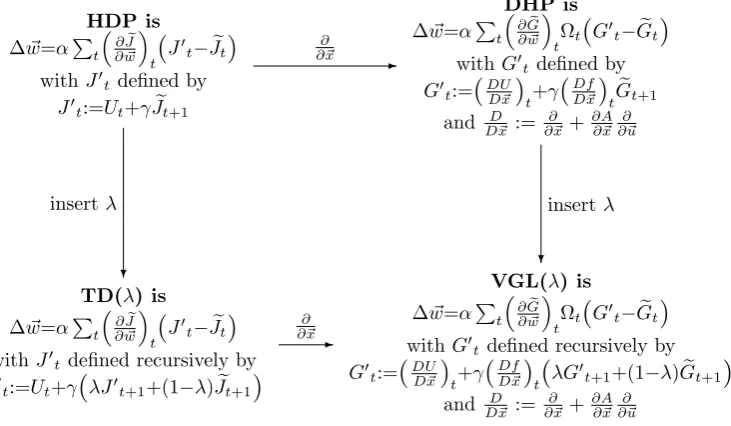
HDP is a value-learning ADP design, i.e. it does not consider value gradients. DHP is

a VGL algorithm. The way these two algorithms are related to each other is shown by the two algorithms at the top of Fig. 1.1.

HDP is

∆w~=αP t

∂Je

∂ ~w

t

(

J 0

t−Jet

)

withJ0tdefined by

J0

t:=Ut+γJet+1

DHP is

∆w~=αP t

∂Ge

∂ ~w

t

Ωt

(

G0t−Get

)

withG0tdefined by

G0t:=

(

DU_D~_x

)

t+γ

(

Df D~x

)

_tGet+1 and D

D~x := ∂ ∂~x+

∂A ∂~x

∂ ∂~u

TD(λ) is

∆w~=αP t

∂Je

∂ ~w

t

(

J0t−Jet

)

withJ0tdefined recursively by

J0t:=Ut+γ

(

λJ0t+1+(1−λ)Jet+1

)

VGL(λ) is

∆w~=αP t

∂Ge

∂ ~w

t

Ωt

(

G0t−Get

)

withG0t defined recursively by

G0t:=

(

DUD~x

)

_t+γ

(

Df D~x

)

_t

(

λG

0

t+1+(1−λ)Get+1

)

and _D~D_x :=_∂~∂_x+∂A_∂~_x_∂~∂_u

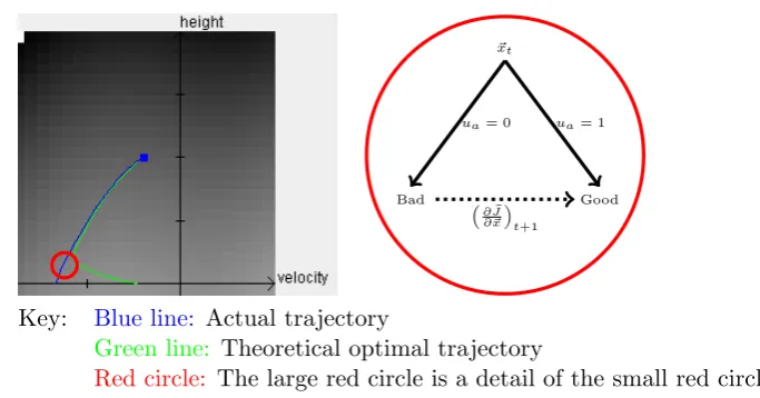
[image:47.595.98.464.333.546.2]

-∂ ∂~x ? insertλ ? insertλ -∂ ∂~x

Figure 1.1: Relationship of VGL(λ) to other ADPRL algorithms.

In this figure, Jeis the output of the critic network Je(~x, ~w), with weight vector w~,

and Ge is the gradient of Jewith respect to the state vector ~x of the agent, i.e. Ge is

the critic’s approximation of the value gradient. The ∆w~ refers to a weight update for the critic neural network, i.e. this shows the main equation of each learning algorithm,

andα >0 is a small learning rate parameter. The subscriptedtindicates the time step of a trajectory, Ut is the instantaneous cost received by the agent at that time step,A

is the output of the action network A(~x, ~e, ~z), and Ωt is an arbitrary positive definite

(48)

1.3 Literature Review

be given in Chapters2-3, but at the moment the figure indicates the key relationships

between various ADPRL algorithms.

The TD(λ) algorithm (Barto et al.,1983;Sutton, 1988) is an extension of HDP to include a constantλ∈[0,1] parameter which specifies how the critic neural network’s output values are to be updated. λ is a blending parameter that specifies how much the critic values are updated towards other critic values (a process known as

“boot-strapping”) as opposed to towards the true total trajectory cost. The exact details of

this blending and the main TD(λ) weight update is shown in the bottom left corner of Fig. 1.1, but again, fuller details will be given in Chapter 2. TD(λ) is a unifying extension between the earlier critic methods, such that TD(1) is equivalent toWidrow

et al. (1974)’s black-jack critic and TD(0) is equivalent to HDP.

From Fig. 1.1, the new algorithm presented by this thesis, VGL(λ), can be shown in context to the other three algorithms. VGL(λ) is most easily understood as an extension of DHP that includes a λparameter analogous to that used in TD(λ). The parameterλ can affect learning speed of the algorithm and convergence stability, and it was the addition of this parameter that led to the convergence proof in Chapter 8,

so it is was an important extension to have made to DHP.

Although best understood as an extension to DHP, the VGL(λ) algorithm was actually derived by changing TD(λ) to learn value gradients, i.e. by following the right-pointing arrow at the bottom of Fig. 1.1. It was the failure of TD(λ) to solve continuous-valued state-space control problems without value exploration, and the slow

speed of its ability to solve them with value exploration, that led to the creation of

VGL(λ) (Fairbank,2008). Examples of these two kinds of difficulties, and the benefits

of VGL methods in solving them, are given in the experiments in the following two

chapters (specifically in Figs. 2.2,3.7and 3.10). It was the understanding that TD(λ) could be defined in this concise form using the recursive definition ofJ0t from Fig. 1.1

that enabled the algorithm VGL(λ) to be defined easily. 1.3.4 Other ADPRL Algorithms

Other variations on the main algorithms shown in Fig. 1.1 are possible. These

in-clude Q-learning and the residual-gradient methods, plus Gradient Temporal

Differ-ences methods. These are described in Sections2.6,2.7.3and 2.7.4, respectively. From

(49)

the same as Q-learning, plus Globalized DHP. These are described in Sections2.6and

3.4.4, respectively. Plus there are other ADP variants including Action Dependent

DHP (ADDHP), Action Dependent GDHP (ADGDHP) and Galerkinized DHP, which

are not described in this thesis, but are described by Prokhorov and Wunsch (1997a)

and Werbos (1998).

Another group of ADPRL algorithms are policy-gradient based methods. These do

not use a critic at all, but instead do direct gradient descent onJb(~x, ~e, ~z) with respect to

the weight vector of the action network,~z. These include the REINFORCE algorithm

byWilliams(1992) and Backpropagation Through Time (“BPPT”) byWerbos(1990a),

and are described in detail in Chapter 6. Despite BPTT being a critic-free method,

BPTT is an essential component of this thesis because a unification proof between

BPTT and the critic-based VGL(λ) algorithm is given in Chapter 8. Since this forms the basis of a convergence proof for one instance of VGL(λ), this link to BPTT makes the most significant theoretical achievement of this thesis.

1.3.5 Convergence Proofs for ADPRL algorithms

Convergence proofs for various RL algorithms exist, but these are mainly for tabular

representations of the critic, or linear function approximation of the critic, and/or fixed

action-networks. These include proofs by Baird (1995); Dayan(1992);Sutton (1988);

Sutton et al. (2000, 2009); Tsitsiklis and Van Roy (1996a). The work of Maei et al.

(2009) is valid for a critic with non-linear function approximation, with a fixed action

network. These works are all described in detail in Section 2.7.

Convergence proofs for the ADP algorithms include work by Al-Tamimi et al.

(2008);Ferrari and Stengel(2004);Heydari and Balakrishnan(2011);Howard(1960b);

Prokhorov and Wunsch(1997b) and these are all described in the introduction of

Chap-ter8.

The critic-free methods, REINFORCE and BPTT, have very good convergence

guarantees with non-linear function approximation and changing action-network

be-haviour, and these convergence results are described further in Chapter 6.

1.4 Model-Free and Model-Based Algorithms

(50)

1.4 Model-Free and Model-Based Algorithms

Model-free algorithms are ones that don’t have an explicit requirement to know

the environment functions,f(~x, ~u, ~e), U(~x, ~u, ~e) or Φ(~x, ~e). These algorithms often do contain instances of the environment functions, but they are included in such a way that

they could represent a robot or agent actually exploring the environment. The agent

could still make deductions about cost received (i.e. U(~x, ~u, ~e)) or state transition made (i.e. f(~x, ~u, ~e)) by pure observation, and without knowledge of the functions themselves. For example the, trajectory-unroll algorithm (Alg. 1.1) is model-free according to this

definition, and so is the TD(λ) weight update, which is defined in Fig. 1.1 and in Chapter2.

In contrast, a model-based algorithm is one which must explicitly know the model

and cost functions. For example, all VGL based algorithms are model based, because

they need to explicitly use the derivatives of the model and cost functions, as can be

seen from their definitions in Fig. 1.1. These derivatives cannot be deduced by single

observations by the agent.

This completes the definition of what distinguishes a model-free algorithm from a

based one. The following two subsections describe the extent to which

model-based and model-free algorithms are used within ADPRL, and which researchers use

which.

1.4.1 Model-Based RL

The sub-field of “model-based RL” is different from the simple classification of an

algorithm as model-based by the above definition.

Kaelbling et al. (1996) define model-based RL as “Learn a model, and use it to

derive a controller.” Model-based RL is also known as “planning in RL” or “indirect

RL” (Sutton and Barto,1998, chap. 9).

When a neural network is trained to learn the model and cost functions using an

appropriate supervised learning method, the neural network will converge (as closely

as possible) to the expectation of the target functions, which will necessarily be

deter-ministic. In this thesis the targets for the deterministic parts of the learned model and

cost functions are denoted with overbar symbols. Using this notation, the model and

(51)

part, so that:

f(~x, ~u, ~e)≡f¯(~x, ~u) +ξf(~x, ~u, ~e)

U(~x, ~u, ~e)≡U¯(~x, ~u) +ξU(~x, ~u, ~e)

Φ(~x, ~e)≡Φ(¯ x~) +ξΦ(~x, ~e).

(1.9)

It is the objective of the model-learning process to achieve, as closely as possible,

¯

f(~x, ~u)≡_E(f(~x, ~u, ~e)) ¯

U(~x, ~u)≡E(U(~x, ~u, ~e))

¯

Φ(~x)≡_E(Φ(~x, ~e)).

(1.10)

If this objective is met then the expectations of the three noise terms, ξf(~x, ~u, ~e),

ξU(~x, ~u, ~e) and ξΦ(~x, ~e) should all be zero.

The three functions ¯f(~x, ~u), ¯U(~x, ~u) and ¯Φ(~x) are all deterministic functions, which is reflected in their notation, since they are not dependent on the noise vector~e. The overbar symbol indicates that they are each expectations of their underlying functions,

i.e. according to Eq. (1.10).

Sutton and Barto (1998) describe an advantage of model-based RL to be that it

makes fuller use of experience, that is it obtains a better policy with fewer environment

interactions, and a disadvantage of model-based RL to be that if the model is not

perfectly learned then the optimization will optimise the wrong model.

Another benefit of model-based RL can be understood by imagining the case of a

robotic flying machine that is to be trained only through the negative reinforcement

of crashes. In this situation it would clearly be beneficial for these crashes to happen

in model-based simulation rather than in reality. This example, when coupled with

the fact that many simulated trajectories can usually be evaluated in the time it takes

a real robot to complete one physical trajectory, makes a strong incentive to choose

model-based methods over model-free ones.

Concerning the disadvantage of using a possibly incorrect learned model, the

model-approximation error is just one more error on top of the model-approximation error in the

critic, and the approximation error in the action network; and as we shall see in Chapter

5, when model-based methods are used it is sometimes possible to remove the action

network, thus removing one layer of approximation error, and hence neutralising this

Value-Gradient Learning

City, University of London Institutional Repository

Citation

:

This is the unspecified version of the paper.

This version of the publication may differ from the final published

version.

Permanent repository link:

Link to published version

:

Copyright and reuse:

City Research Online aims to make research

outputs of City, University of London available to a wider audience.

Copyright and Moral Rights remain with the author(s) and/or copyright

holders. URLs from City Research Online may be freely distributed and

linked to.

Value-Gradient Learning

Michael Fairbank

Contents

List of Figures

List of Tables

List of Algorithms

Acknowledgements

Declaration

Abstract

Glossary

Part I

Chapter 1

Introduction

1.1

Motivation and Challenges

1.2

Formal Specification of the ADPRL Optimisation

Prob-lem

1.3

Literature Review

(

)

(

)

(

)

(

)

(

)

(

)

(

)

(

)

(

)

(

)

1.4

Model-Free and Model-Based Algorithms