Temporal correlations in social multiplex networks

City, University of London Institutional Repository

Citation:

Starnini, M., Baronchelli, A. & Pastor-Satorras, R. (2016). Temporal correlations

in social multiplex networks. .,

This is the draft version of the paper.

This version of the publication may differ from the final published

version.

Permanent repository link:

http://openaccess.city.ac.uk/14938/

Link to published version:

Copyright and reuse: City Research Online aims to make research

outputs of City, University of London available to a wider audience.

Copyright and Moral Rights remain with the author(s) and/or copyright

holders. URLs from City Research Online may be freely distributed and

linked to.

City Research Online:

http://openaccess.city.ac.uk/

[email protected]

Michele Starnini,1 Andrea Baronchelli,2 and Romualdo Pastor-Satorras3

1

Departament de F´ısica Fonamental, Universitat de Barcelona, Mart´ı i Franqu`es 1, 08028 Barcelona, Spain

2_{Department of Mathematics, City University London, Northampton Square, London EC1V 0HB, UK} 3

Departament de F´ısica, Universitat Polit`ecnica de Catalunya, Campus Nord B4, 08034 Barcelona, Spain

Social interactions are composite, involve different communication layers and evolve in time. However, a rigorous analysis of the whole complexity of social networks has been hindered so far by lack of suitable data. Here we consider both the multi-layer and dynamic nature of social relations by analysing a diverse set of empiricaltemporal multiplex networks. We focus on the measurement and characterization of inter-layer correlations to investigate how activity in one layer affects social acts in another layer. We define observables able to detect when genuine correlations are present in empirical data, and single out spurious correlation induced by the bursty nature of human dynamics. We show that such temporal correlations do exist in social interactions where they act to depress the tendency to concentrate long stretches of activity on the same layer and imply some amount of potential predictability in the connection patterns between layers. Our work sets up a general framework to measure temporal correlations in multiplex networks, and we anticipate that it will be of interest to researchers in a broad array of fields.

INTRODUCTION

The study of social networks1_{, originally focused at reveling the hidden structures of social organizations}2_{, has been}

recently revamped by the availability of large digital databases3_{. Complex networks defined by social interactions are}

in fact the natural environment for dynamical processes4, such as the spread of biological diseases5, the formation of opinions and consensus6 or the spread of rumors and fads7. Initial studies of social interaction patterns in terms of complex networks mostly considered a simple mapping to a static graph structure, in which nodes represent individuals, while edges stand for pairwise (directed, undirected or weighted3_{) social interactions}1,8_{. This approach}

led to successful research and rich conclusions but neglects two main aspects of real-world social interaction, namely that social interactions

1. are diverse in nature and quality, with different layers co-exististing and interacting with one another (e.g., physical vs. digital interactions)9;

2. evolve in time, with new relationship continuously being created and destroyed.

The first point indicates that patterns of social interactions are more naturally described in terms of multiplex

networks10–12, composed by nodes connected by edges belonging to different layers corresponding to the different interaction channels. New observables such as multilayer clustering, degree correlations or layer overlap10 have al-lowed for a better characterization of social networks and helped clarify the behavior of dynamical processes such as random walks,13_{, percolation}14 _{or epidemic spreading}15,16 _{on these structures. The second point has led to a more}

realistic representation of social networks in terms of temporal networks17,18_{, in which edges (and even nodes) are}

dynamic entities that evolve in time. Taking into account the temporal dimension has allowed to uncover unexpected properties of social dynamics such as its bursty nature, characterized by a heavy-tailed distribution of inter-event times τ between consecutive interactions19,20_{, often compatible con power-law forms, ψ(τ) ∼ τ}−1−α_{. Temporal}

effects, moreover, radically alter the properties of dynamical processes on such evolving networks21–24_.

In this paper we take into account the full complexity of social networks and present an empirical analysis in which such structures are described astemporal multiplex networks, i.e., networks with a given set of nodes whose edges (1) belong to different layers (representing different kinds of interactions)and (2) have an intrinsic dynamics of creation and annihilation (see Fig. 1). We consider various scenarios: human contact networks, recorded by the “Reality Mining” (RM) experiment25_{and consisting of two independent data sets, ”Social Evolution” (SE) and “Friends and}

Family” (FF); Open Source Software (OSS) collaboration networks26_{, with data provided by a OSS project part of}

the Apache software foundation27_{; and scientific collaboration networks}28_{, reconstructed from the American Physical}

Society (APS) data sets for research29. RM contact networks are formed by a physical layer of proximity, face-to-face (f2f) contacts and a virtual layer of digital contacts (phone calls and text messages) between individuals; OSS collaboration networks consist of a communication layer (emails) and a co-work layer (commit code to the same file) between developers; in APS collaboration networks we distinguish two layers formed by co-authorship of papers published in the journal Physical Review Letters (PRL) and papers published in journals different form PRL. See Methods and Supplementary Information a full description of the data sets considered.

We focus on the temporal correlations between social activity taking place on the different layers investigating if and how a social interaction taking place at some given layer may alter the probability of a subsequent interaction at a different layer. We show that inter-layer correlations do exist in social temporal multiplex networks, and we demon-strate their effect in two main features. Firstly, they reduce the length of stretches of uninterrupted interactions in the same layer that should be expected from bursty uncorrelated activity on isolated layers, by inducing amultitasking

or switching effect. Secondly, they induce a certain degree of predictability in the interaction patterns, in the sense that the sequence of contacts of an agent in a given layer is affected by her previous contacts in another layer.

RESULTS

A mathematical description of multiplex temporal networks

Temporal multiplex networks can be mathematically described by endowing the multiplex paradigm10 _{with an}

additional temporal dimension30_{. In this way, a temporal multiplex network can be represented by acontact sequence,}

a set of quadruplets (i, j, t, `) indicating that nodesiandjare connected at timetin layer`, withi, j∈ V ={1, . . . , N}, the set of nodes, of a total number |V|=N,t ∈ T the set of contact times, and `∈ L={`1, `2, . . . , `L}, the set of

|L|=Llayers.

a)

b)

t

t

t

c)

t

t

t

d)

Figure 1: Different observation levels of a temporal multiplex network. A full temporal multiplex network (a), in this case with two levels, is represented by different snapshots at timesti∈[0, T] of a single set of nodes with edges on different layers (colors) that appear at different times. The integrated static multiplex (b) is given by the projection over the time window [0, T] of all edges, which appear in their respective layers if they have appeared at least once in the whole observation window. A single layer temporal network (c) is obtained by projecting all layers onto a single one. Simultaneous projection

over time and layers leads to a single layer static network (d).

obtained by projecting different layers`onto a single aggregate layer for each contact timet∈ T, so that the resulting temporal network is described in terms of a contact sequence with triplets (i, j, t). A static multiplex network is recovered by projecting time t onto a time-aggregated network for each layer `, resulting in a set of L (possibly weighted) networks, G~ = (G`1, G`2, . . . , G`L). Each network G` is described by the adjacency matrix

3 _a`_{, whose}

elements a`

ij =w`ij =

P

tχ(i, j, t, `) represent the number of interactions between i and j occurring over the whole

contact sequence in layer`. One can project both timet and multiplexity ` onto a time-aggregated, single-layered network G. The elements of its adjacency matrix aij =wij =P`,tχ(i, j, t, `) represent the number of interactions

betweeniandj occurring over the whole contact sequence across any layer`.

For the sake of simplicity, in the following we will be mainly concerned in the analysis of temporal multiplex networks formed by only two layers (i.e. a duplex), that will be arbitrarily denoted asup (`= +1) anddown (`=−1).

Measuring inter-layer correlations

Inter-layer temporal correlations correspond to the possibility that interactions taking place on one layer have an effect on the occurrence of interactions on other layers, either increasing or depressing their probability. We represent the full structure of the temporal multiplex network in terms of multivariate point processes31_{, i.e. a collection of}

random processes consisting in a set of isolatedpoints, representing the interactions between individuals, taking place at random positions in time. For each layer`, we can adopt three different levels of description:

1. A single point process,p`, in which a point corresponds to an interaction of an individual in layer`, regardless

of the involved individuals;

2. A set of N point processes, {p`,i}i∈V, in which a point corresponds to an interaction of an agent i with any

other agent in the same layer;

3. A set ofE`point processes,{p`,i,j}i,j∈V, in which a point corresponds to an interaction of agentiwith agentj

in the same layer, andE` is the number of edges in layer`.

The simplest characterization of these point processes is in terms of their inter-event time distributions representing the probability that two points in a process are separated by a timeτ. The temporal multiplex networks under consid-eration show an interevent time distribution between consecutive interactions of a single individual,ψ`(τ), compatible

with a power-law, ψ`(τ) ∼τ−(1+α`), with similar exponent α` between layers (see Supplementary Information and

Supplementary Figure 5). Therefore, an uncorrelated null model in terms of point processes corresponds to L (or

N×L, or P

`E`) uncorrelated renewal processes32, depending on the level of coarse-graning we choose to consider,

100 101 102 103 104 10-6

10-4 10-2 100

100 101 102 103 10-6

10-4 10-2 100

100 101 102 103 10-6

10-4 10-2 100

100 101 102 10-4

10-2 100

I= 2.3

P= 1.8 P= 2.1

I= 1.9

n

P

(

n

)

SE

OSS

Ind

ivi

dua

ls

Pa

irs

100 101 102 103 104 10-6

10-4 10-2 100

100 101 102 103 10-6

10-4 10-2 100

100 101 102 103 10-6

10-4 10-2 100

100 101 102 10-4

10-2 100

`= +1

`= +1(NM)

`= 1

`= 1(NM)

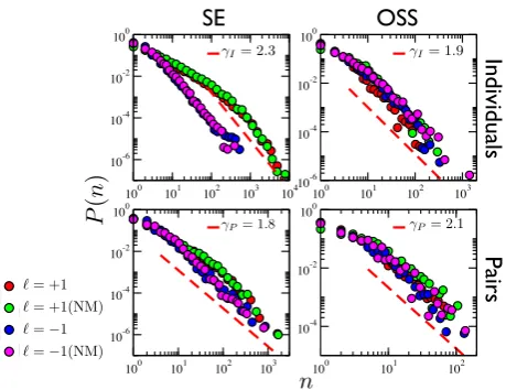
Figure 2: Sequence of consecutive interactions on the same layer. Probability of finding a numbern of consecutive interactions occurring on the same layer `, not interrupted by interactions on the other layer, P`(n), for different data sets considered and for the corresponding data randomized according the null model (NM). Probability distribution P`(n) for aggregated point processes constituted by the interactions of a single individuals (top panels) and a pair of individuals (bottom panels). Power-law decays,P`(n)∼n−γ, with different exponent for pairs,γP, and individuals,γI, are plotted in dashed line.

Data shown are, from left to right: RM contact networks, data set SE, and OSS collaboration network.

The point processes mapping social interactions are non-stationary as the inter-event time distributions follow a power law form with an exponentαin general smaller than one, and therefore with a diverging first moment, typical of non-Markovian dynamics33_{. However, standard techniques to detect the presence of correlations between related}

point processes, such as the cross-correlation function, the spike distance measurements34, and the Ripley K function35 are mainly aimed at exploring the properties of stationary signals, i.e., processes that do not change when shifted in time. Therefore, new quantities able to capture the possible presence of temporal correlations between the layers of temporal multiplex networks are needed. We discuss several possibilities below.

Sequence of consecutive interactions within the same layer

A simple observable able to quantify the presence of correlated behavior between different layers is the distribution

P`(n) of the numbernof consecutive events occurring within the same layer`, not interrupted by any event occurring

on other layers `0 6= `. The presence of large sequences of interactions occurring on one layer may be associated to reinforcement mechanisms within the same layer. On the contrary, assuming lack of inter-layer correlations, one would expect that continuous bursts of activity in the same layer tend to be interrupted by activity in other layers, leading to bounded (exponential) distributionsP`(n) of consecutive events in layer`. In support of this picture, the

analysis of uncorrelated multivariate Poisson point processes indicates the presence of exponential distributionsP`(n),

see Supplementary Information.

Fig. 2 shows the empirical probability distribution P`(n) computed from the SE contact and OS collaboration

networks (see Supplementary Fig. 6 for the FF and APS datasets). Point processes constituted both by the interactions of single individuals i in a layer `, {p`,i}, and by the interactions of a pair individuals iand j in a layer `, {p`,i,j}

are shown. In all casesP`(n) is broad tailed and compatible with a power law,P`(n)∼n−γ. The exponent depends

on considered data set, is slightly different between point processes constituted by individuals,γI, or pairs, γP (with

the exception of APS networks, see Supplementary Fig. 6, probably due to the scarcity of pairs of scientists with intense activity), and appears to be independent on the layer considered. The presence of uninterrupted sequences of consecutive interactions in the same layer might be interpreted as consequence of temporal correlations between layers, with interactions of one kind depressing interactions of the other kind. For example, it could be speculated that the tendency of an individual to relate with other peers through f2f contacts may reduce his probability to interact with them through calls or texts. However, this interpretation does not take into account the role played by the burstiness of social interactions. Indeed, the presence in both layers of a broad tailed interevent time distribution,ψ(τ) represents a sufficient condition for the observed shape of P`(n), even if the layers are completely uncorrelated. Specifically,

SE

OSS

Di

stri

buti

on

Sca

tter

-0.5 -0.4 -0.3 -0.2 -0.1 0.0 0.00

0.05 0.10 0.15 0.20 0.25

∆t = 103

∆t = 103 (NM)

∆t = 104 ∆t = 104 (NM)

-0.8 -0.6 -0.4 -0.2 0.0 0.2 0.00

0.10 0.20 0.30 0.40

∆t = 104

∆t = 104 (NM)

∆t = 105

∆t = 105 (NM)

-0.4 -0.2 0.0

-0.4 -0.2

0.0 ∆t = 10 3

∆t = 104

-0.8 -0.6 -0.4 -0.2 0.0 0.2 -0.8

-0.6 -0.4 -0.2 0.0

0.2 ∆t = 10

4

∆t = 105

P

(

r

)

r

r

r

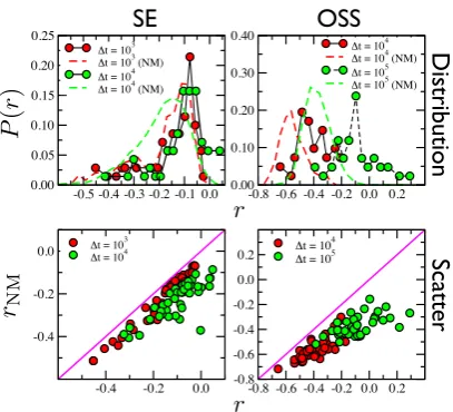
Figure 3: Multitasking index of individuals. Comparison of the multitasking index of the original data, r, with the corresponding index rN M of data randomized according the null model. Probability distribution of the multitasking index of the original and randomized data, P(r) and P(rN M) (top row), and scatter plot of the multitasking index of the original versus randomized data,rvs. rN M (bottom row), for different time window ∆tand different data sets. In scatter plots, only individuals withrwith a p-value smaller than 0.05 or greater than 0.95 with respect to the null model are plotted. Data shown are, from left to right: RM contact networks, data sets SE and FF (∆texpressed in seconds), OSS collaboration network and

APS collaboration network (∆texpressed in days).

by any event of the other series, will follow a power-law form,P`(n)∼n−1−α−`/α` (see Supplementary Information).

Thus, the sequences of consecutive events of the same kind observed in the data is explained by the bursty nature of social acts. This fact is confirmed by a comparison of the original data with a null model which randomizes the multiplex networks by completely washing out temporal correlations between layers, but separately preserving the interevent time distribution ψ`(τ) of each layer (see Supplementary Information). Fig. 2 (see also Supplementary

Fig. 6) shows that there is no significant difference between original and randomized data, and indicates that the long tailed form of the distribution of consecutive interactions does not represent a signature of inter-layer correlations.

Multitasking index of individuals

Another helpful observable is obtained by comparing the number of interactions, n`(∆t) and n−`(∆t), that an

individual performs in a time interval ∆tin two different layers`and−`. Amultitasking index ri(∆t) of individuali

can be defined as the Pearson correlation coefficient between the set of variables{n`(∆t), n−`(∆t)}, where each pair

(n`(∆t), n−`(∆t)) is measured in layers ` and −` at different time intervals of fixed length ∆t. If ri(∆t) is grater

than zero (i.e. if the values ofn`(∆t) andn−`(∆t) attain comparable values in the time window), then individualiis

simply distributing his activity among the two layers and he/she is likely to interact indistinctly in both layers at the same time; on the contrary, ifri(∆t))<0 (i.e. if a largen`(∆t) is associated with a smalln−`(∆t), and vice-versa in

the same time window), then he/she is likely to be concentrating her activity on one of the two layers.

Fig. 3 (top row) shows the probability distribution of the multitasking index r(∆t), P(r), measured for each node of the SE contact and OS collaboration networks (see Supplementary Fig. 7 for the FF and APS datasets), for different values of the time interval ∆t, obtained by cutting the whole temporal sequence into consecutive slices. The multitatsking index is generally negative, for every data set considered. This result is in agreement with the presence of large sequences of uninterrupted social acts of the same kind discussed in the previous section. In a given time interval ∆t, an individual is more likely to relate with the others only through face-to-face interactions, or only through calls or texts, and less likely to use both channels equally. In the context of the OSS collaboration network, this translates into developers more likely either to communicate or to co-work, not doing both actions at the same time. In APS networks, see Supplementary Fig. SM-3, it implies that authors are more likely to collaborate in a sequence of papers in the same journal, instead of switching among different journals. As expected, a larger time window ∆tthe anti-correlation is mitigated by large time windows of observation.

corresponding coefficientr_iN M(∆t) obtained by randomizing the original data according to the null model preserving the interevent time distributions. Fig. 3, bottom row (see also Supplementary Fig. 7), shows a scatter plot between coefficientsr(∆t) andrN M(∆t), for each node of the contact and collaboration networks, for different time intervals

∆t. Only individuals whose coefficientr(∆t) is significantly different fromrN M(∆t) (with a p-value smaller than 0.05

or greater than 0.95, see Supplementary Information) are plotted. One can see that almost all significant individuals have a multitasking coefficientr(∆t) greater than the corresponding coefficientrN M(∆t) obtained in the null model,

as highlighted by the diagonal line. The only partial exception is the APS collaboration network, where the majority of scientists fulfillr(∆t)> rN M(∆t), while few of them follow the opposite behavior.

As a further check, the right plot of Supplementary Fig. 7 also shows the coefficients rs_{(∆t) and r}s

N M(∆t) of a

synthetic temporal multiplex network generated by uncorrelated layers (see Supplementary Information), of the same size of the APS collaboration network. Only few nodes (less than 0.1%) have a multitasking coefficientrsignificantly different from the one obtained in the null model, rN M, and they are equally distributed between a group with r < rN M and another group withr > rN M. Thus, a broad tailed interevent time distribution alone is not a sufficient

condition to explain the values of the multitasking coefficient found in real social networks.

Influence and predictability between layers

Temporal correlations between layers may lead to a certain degree of predictability in terms of influence of the interactions in one layer on the interactions on the other one. Let us consider a case in which an individualiswitches from one kind of interaction to another one, e.g. s/he sends an email to a colleague and then he co-edits some code with another collaborator. This is represented with a link between node i and node j in layer `1 at time t1 and a

link between node iand nodek (including the case j=k) in layer `2 at timet2, witht1< t2 or viceversa. We are

interested in understanding if an individual i, after having an interaction with individual j in layer `1, chooses his

next partnerkin layer`2 at random, or if there is a certain degree of predictability in his choice.

We address this issue with an entropy and mutual information analysis, widely used to capture the randomness of sequences of events, and to extract its degree of predictability in, e.g. , human mobility36_{, conversation patterns}37 _or

online games38. The uncorrelated entropyH_iu(`) of individuali in layer`is defined as

H_iu(`) =−X

j`

pi(j`) ln[pi(j`)], (1)

wherepi(j`) is the probability that individualiinteracts with individual j in layer`. The uncorrelated entropy thus

measures the degree of heterogeneity in the interactions pattern of an individual in one layer. If individuali relates much more with some of his peers with respect to others in layer`, thenHu

i(`) will be small; instead, if he interacts

equally with all his contacts, thenH_iu(`) will be large.

The conditional entropyH_ic(`→ −`) of individualifrom layer`to layer−`is defined as

H_ic(`→ −`) =−X

j` pi(j`)

X

k−`

pi(k−`|j`) ln[pi(k−`|j`)], (2)

where pi(k−`|j`) is the conditional probability that individual iinteracts with individual k in layer −` immediately

after interacting with individual j in layer `. The conditional entropy, thus, takes into account the influence of one layer on the other one. If an interaction of an individuali withj in layer` is likely to prompt a specific interaction with individualkon layer−`, then the conditional entropy will be small, otherwise if the interaction pattern between layers is random, it will be large.

We quantify the predictability of layer−`due to the influence of layer`by the mutual information, defined for each individual i as the difference between uncorrelated and conditional entropy, Ii(` → −`) = Hiu(−`)−Hic(` → −`),

thus

Ii(`→ −`) =

X

j`,k−`

pi(j`, k−`) ln

_p

i(j`, k−`) pi(j`)pi(k−`)

, (3)

wherepi(k−`, j`) is the joint probability that individualiinteracts first with individualkin a layer−`and immediately

after with individualj in a layer`. Since it holds thatHu

i ≥Hic, the mutual informationIi is always positive, and it

is equal to zero only if the interaction patterns of individualion the two layers−`and`are temporally uncorrelated. Therefore,Ii(`→ −`) measures the degree of predictability of the interaction pattern of individualiin layer−`, and

SE

OSS

M

utua

l

Inf

orma

tio

n

Entr

op

y

0.0 0.5 1.0 1.5 2.0 2.5 3.0 0.0

0.5 1.0 1.5 2.0 2.5 3.0

0.0 0.5 1.0 1.5 2.0 2.5 3.0 0.0

0.5 1.0 1.5 2.0 2.5 3.0

0.0 1.0 2.0 3.0 4.0 5.0 6.0 0.0

1.0 2.0 3.0 4.0 5.0 6.0

0.0 1.0 2.0 3.0 4.0 5.0 6.0 0.0

1.0 2.0 3.0 4.0 5.0 6.0

Hu Hc

Hu( 1) vsHc(+1! 1)

Hu(+1) vsHc( 1!+1)

I( 1_!+1)

I

(+1

!

1)

Figure 4: Entropy and mutual information between layers. Scatter plots of the uncorrelated vs conditional entropy of individuali(bottom row),Hiu(`) vsHic(`→ −`), and mutual information between layers, Ii(+1→ −1) vsIi(−1→+1), for different data sets. Only individuals with a conditional entropy with a p-value smaller than 0.05 with respect to the null model

are plotted. Data shown are, from left to right: RM contact networks, data set SE, and OSS collaboration network.

Fig. 4 (bottom panels) shows the relation between uncorrelated and conditional entropy of each individuali, on the SE contact and OS collaboration networks (see Supplementary Figure 8 for the FF and APS datasets). To avoid spurious effects due sample size issues, we perform a bootstrap analysis (see Supplementary Information), retaining only those individuals who have a value of the conditional entropy significantly smaller than the one obtained by rewiring the network according to a null model, which destroys inter-layer temporal correlations. One can see that several individuals show a significant entropy difference, resulting in a certain degree of predictability, in each data set under consideration. For the case of RM contact networks, data set SE has a greater number of individuals with a significant entropy difference, with larger values of the conditional entropyHc

i and mutual informationIi, with respect

to data set FF, probably due to its larger duration T (see Supplementary Table I). For both data sets FF and SE, the uncorrelated and conditional entropy obtained in the physical layer (`= +1) are larger than the ones obtained in digital layer (`=−1), because the former is characterized by a richer pattern of interactions, with a larger density and heterogeneity (see Supplementary Table I). The same behavior is observed in the OSS collaboration network, with the more dense communication layer (` =−1) shows larger values of the uncorrelated and conditional entropy than the ones obtained in co-work layer (` = +1). On the contrary, in the APS collaboration network the layers have a similar densities, and show similar entropy values. Fig. 4 (top panels), see also Supplementary Fig. 8, shows the relation between the predictability of an individual i in layer ` =−1 obtained by layer ` = +1, Ii(+1 → −1),

and viceversa,Ii(−1 →+1). One can see that there is no dominant pattern of influence between layers. For some

individuals interactions in layer`= +1 influences interactions on the other`=−1,I(+1→ −1)>0, for some others the opposite is true, I(−1 → +1) >0, and for many individuals there is a mutual influence between layers, both

I(+1→ −1)>0 andI(−1→+1)>0.

Discussion

In this paper we have considered, for the first time together, both the temporal and multiplex dimensions of real social networks. We have concentrated on how the activity an individual shows in one layer influences her behaviour on the other. We have proposed different measures of increased complexity, pointing out that the bursty human activity within each layer is responsible for spurious inter-layer correlations. More careful analysis based on the multitasking index we have introduced show that temporal correlations between layers are actually present in multiplex networks, and that their effect in general is to reduce the tendency of individuals to engage in large sequences of interactions within the same layer, which is the natural outcome of the broad tailed form of the interevent time distribution. Finally, we have addressed the mutual influence that layers exert on each other. While we showed that there is a clear signature of mutual influence between the activity on different layers, the analysis of our datasets seems to indicate that the precise nature of this influence shows a large variability across individuals.

and mutiplex properties of social networks. On the other hand, in doing so we have proposed a number of measures able to reveal the presence and nature of inter-layer temporal correlations on any tipe of time-varying multiplex networks. We therefore expect the results presented here to be relevant for the wide community of researchers interested in Social Systems and, more broadly, Network Science.

Acknowledgements We thank Prof. Vladimir Filkov for sharing the data of the Open Source Software networks. M.S. acknowledges financial support from the James S. McDonnell Foundation. R.P.-S. acknowledges financial support from the Spanish MINECO under project No. FIS2013-47282-C2-2, and ICREA Academia, funded by the Generalitat de Catalunya.

Appendix: Empirical data

We consider three different kinds of empirical temporal multiplex networks, all formed by two layers (duplex): human contact networks, recorded by the RM experiment25, OSS collaboration networks, reconstructed by means of data provided by the Apache software foundation27, and scientific collaboration networks, reconstructed by means of the APS data set for research29_{. The RM experiment}25 _{is conducted by the MIT Media Lab and composed by}

data sets ”Social Evolution” (SE) and ”Friends and Family” (FF). It records proximity data by means bluetooth sensors, forming a layer of physical interactions,`= +1, and digital communications, as given by phone calls and text messages, merged in a layer of digital interactions`=−1. The Apache software foundation27 provides data of email communications between developers and their commits to edit files of several OSS project. We focus on “Apache Axis2/Java, one of the project involving the largest number of developers, and consider a layer of co-work,`= +1, formed by co-commits to edit the same file, and a layer of communication, `=−1, formed by email messages. The APS dataset29 _{provides information about all papers published by the APS since 1893. A multiplex network can}

be constructed by considering the co-authorship of a paper published in any of the APS journals. We consider a layer formed by co-authorship in the journal Physical Review Letters (PRL),`= +1, and coauthorship in other APS journal, excluding PRL,`=−1.

1 _{M. Jackson,Social and economic networks (Princeton University Press, 2010).} 2

J. L. Moreno,Who shall survive? (Beacon House Inc., Beacon N. Y., 1953), 2nd ed. 3

M. E. J. Newman,Networks: An introduction (Oxford University Press, Oxford, 2010).

4 _{A. Barrat, M. Barth´elemy, and A. Vespignani, Dynamical Processes on Complex Networks (Cambridge University Press,}

Cambridge, 2008). 5

R. Pastor-Satorras, C. Castellano, P. Van Mieghem, and A. Vespignani, Rev. Mod. Phys.87, 925 (2015). 6 _{P. Sen and B. K. Chakrabarti,Sociophysics: An Introduction (Oxford University Press, Oxford (UK), 2013).} 7 _{J. Leskovec, L. A. Adamic, and B. A. Huberman, ACM Trans. Web1, 5 (2007), ISSN 1559-1131.}

8

S. Wasserman and K. Faust,Social Network Analysis: Methods and Applications(Cambridge University Press, Cambridge, 1994).

9 _{L. M. Verbrugge, Social Forces57, 1286 (1979), http://sf.oxfordjournals.org/content/57/4/1286.full.pdf+html, URLhttp:}

//sf.oxfordjournals.org/content/57/4/1286.abstract.

10

S. Boccaletti, G. Bianconi, R. Criado, C. del Genio, J. G´omez-Garde˜nes, M. Romance, I. Sendi˜na-Nadal, Z. Wang, and M. Zanin, Physics Reports544, 1 (2014), ISSN 0370-1573.

11

M. Kivel¨a, A. Arenas, M. Barth´elemy, J. P. Gleeson, Y. Moreno, and M. A. Porter, J. Complex Networks2, 203 (2014). 12

K.-M. Lee, B. Min, and K.-I. Goh, Eur. Phys. J. B88, 48 (2015), ISSN 1434-6028, 1502.03909, URLhttp://link.springer.

com/10.1140/epjb/e2015-50742-1.

13

M. De Domenico, A. Sol´e-Ribalta, S. G´omez, and A. Arenas, Proceedings of the National Academy of Sciences111, 8351 (2014), ISSN 0027-8424, 1306.0519, URLhttp://dx.doi.org/10.1073/pnas.1318469111.

14 _{S. V. Buldyrev, R. Parshani, G. Paul, H. E. Stanley, and S. Havlin, Nature464, 1025 (2010).} 15

O. Yagan, D. Qian, J. Zhang, and D. Cochran, Selected Areas in Communications, IEEE Journal on31, 1038 (2013), ISSN 0733-8716.

16 _{M. Dickison, S. Havlin, and H. E. Stanley, Physical Review E85, 066109 (2012).} 17 _{P. Holme and J. Saram¨aki, Physics Reports519, 97 (2012).}

18

P. Holme, Eur. Phys. J. B88, 234 (2015), ISSN 1434-6028, arXiv:1508.01303v1, URLhttp://link.springer.com/10.1140/

epjb/e2015-60657-4.

19 _{J. G. Oliveira and A.-L. Barabasi, Nature437, 1251 (2005).} 20

J. Stehl´e, N. Voirin, A. Barrat, C. Cattuto, L. Isella, J.-F. Pinton, M. Quaggiotto, W. Van den Broeck, C. R´egis, B. Lina, et al., PLoS ONE6, e23176 (2011).

21 _{M. Kivela, R. Kumar Pan, K. Kaski, J. Kertesz, J. Saramaki, and M. Karsai, J. Stat. Mech. p. P03005 (2012).}

22

23

A. Vazquez, B. R´acz, A. Luk´acs, and A.-L. Barab´asi, Phys. Rev. Lett.98, 158702 (2007).

24 _{R. Parshani, M. Dickison, R. Cohen, H. E. Stanley, and S. Havlin, EPL (Europhysics Letters)90, 38004 (2010).} 25 _{N. Eagle and A. Pentland, Personal and Ubiquitous Computing10, 255 (2006).}

26

Q. Xuan, H. Fang, C. Fu, and V. Filkov, Phys. Rev. E 91, 052813 (2015), URL http://link.aps.org/doi/10.1103/

PhysRevE.91.052813.

27 _{(????), URLhttp://www.apache.org/.} 28

M. E. J. Newman, Proc. Natl. Acad. Sci. USA98, 404 (2001). 29

American Physical Society. Data sets for research.(2013), URLhttps://publish.aps.org/datasets. 30 _{M. Starnini, A. Baronchelli, A. Barrat, and R. Pastor-Satorras, Phys. Rev. E85, 056115 (2012).} 31

D. Cox and V. Isham,Point Processes, Chapman & Hall/CRC Monographs on Statistics & Applied Probability (Taylor & Francis, Cambridge, U.K., 1980), ISBN 9780412219108.

32 _{D. R. Cox,Renewal Theory(Methuen, London, 1967).} 33

J. H. P. Schulz, E. Barkai, and R. Metzler, Phys. Rev. X4, 011028 (2014), ISSN 2160-3308. 34

M. C. W. van Rossum, Neural Computation13, 751 (2001).

35 _{B. D. Ripley, Spatial statistics, Wiley series in probability and mathematical statistics (J. Wiley & Sons, Hoboken, NJ,}

1981), ISBN 0-471-08367-4, includes indexes. 36

C. Song, Z. Qu, N. Blumm, and A.-L. Barab´asi, Science327, 1018 (2010), ISSN 0036-8075. 37 _{T. Takaguchi, M. Nakamura, N. Sato, K. Yano, and N. Masuda, Phys. Rev. X1, 011008 (2011).} 38 _{M. Szell, R. Sinatra, G. Petri, S. Thurner, and V. Latora, Sci. Rep.2, 457 (2012).}

39

J. Kingman,Poisson Processes, Oxford Studies in Probability (Clarendon Press, Oxford, 1992), ISBN 9780191591242. 40

SUPPLEMENTARY INFORMATION

I. DETAILED DESCRIPTION OF THE EMPIRICAL DATASETS

A. RM contact network

The “Reality Mining” experiment provides two different data sets, both involving different groups of individuals interacting daily for a large period: “Friends and Family” (FF), involving a family residential adjacent to a university in the US, and “Social Evolution” (SE) performed on an undergraduate dormitory. Both provide data of three different kinds of social interactions: proximity or face-to-face (f2f) contacts, recorded by Bluetooth (BT) sensors, and phone calls, and text messages. Each data set is represented by a temporal duplex network, constituted by two different layers: a physical layer (`= +1), formed by f2f interactions, and a digital layer (`=−1), built by merging phone calls and text messages data. In order to reconstruct the multiplex network, we select only those individuals interacting in both layers. In calculating the multitasking index, we consider only those individuals with at 10 interactions in each layer.

Proximity interactions are recorded by BT technology every 5 minutes, while phone calls and text messages timing is recorded with precision of one second. We note that f2f interactions are not recorded exactly every 5 minutes, but there is a dispersion around this value. Therefore, we consider that a f2f contact between individuals iand j is interrupted if and only if the gap time between two consecutive records of an interactions betweeniandj is greater than 10 minutes. Since the resolutions of physical and digital contacts are considerably different (1 second versus 300 seconds or more), we decide not to aggregate interactions over an elementary time step. This choice ensures no data loss, given that aggregating calls and texts over a time window of 300 seconds (the proximity interactions time scale) would have lead to lost bursts of short-term interactions, a typical feature of the digital layer (e.g. bursts of text messages exchanged between a pair of individuals within a short time window). We consider the links formed by text messages as bidirectional, and neglect the temporal duration of interactions, representing social interactions as point-like events occurring at the first instant of their duration.

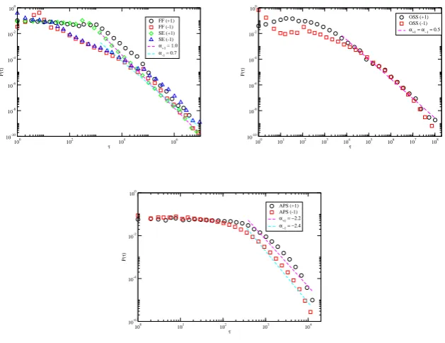
The main average properties of the FF and SE data sets are summarized in Table I. FF and SE have a similar number of nodesN, and a very large durationT: Data set SE, in particular, covers the full academic year 2008/2009 and it is much longer than data set FF. Fig. 5 shows that the distribution of gap times τ between consecutive interactions of an individuals within the same layer`, ψ`(τ), is compatible with a power law,ψ`(τ)∼τ−(1+α`). The

exponent α` is similar between physical (`= +1) and digital (`= +1) layer,α+1= 1.0 andα−1 = 0.7, and notably

it is the same between data sets FF and SE. Note that in the physical layer (`= +1) interevent gap times are larger than the minimum interval between consecutive interactions between the same pair, equal to 600 seconds. Since the large durationT, the aggregated multiplex network has a large average strengthhsi, which means that the links have a large weight, i.e. each pair of individuals interact many times. The physical layer is much more dense than the digital one, and the overlap O between them is very large, almost all links of the digital layer are present in the physical layer.

Interaction Data set Start date N T O Layer` E hki hsi

Contact

SE 27/09/2008 73 242 d 255 Phys. `= +1 2422 66.4 25803 Virt. `=−1 261 7.15 354

FF 19/10/2010 74 156 d 122 Phys. `= +1 1958 52.9 10725 Virt. `=−1 143 3.86 575

Collaboration

OSS 04/10/2001 52 11 y 237 Work`= +1 256 9.85 184 Comm.`=−1 647 24.9 398

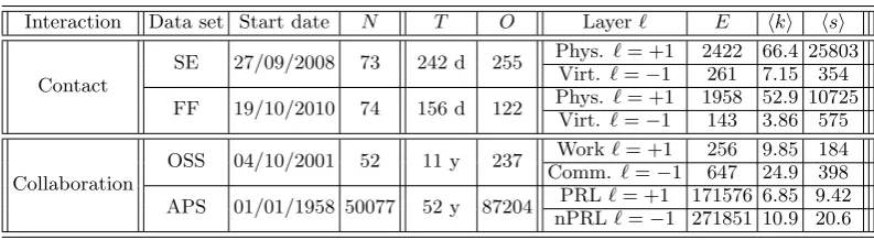
APS 01/01/1958 50077 52 y 87204 PRL`= +1 171576 6.85 9.42 nPRL`=−1 271851 10.9 20.6

Table I: Some properties of the temporal multiplex networks under consideration, the RM contact networks, constituted by data sets FF and SE, and the OSS and APS collaboration network. Properties shown are: Kind of social interaction (contact or collaboration); type of data set; starting date;N, number of nodes of the network;T, duration of the temporal network (in days for the contact networks and years for the collaboration network);O, overlap between layers in the aggregated multiplex; layer considered, `=±1;E number of edges in each layer of the aggregated multiplex; hki` =N−1P_ik`i average degree of

each layer`of the aggregated multiplex;hsi`=N−1Pijw `

100

102

104

106

τ

10-10

10-8

10-6

10-4

10-2

100

P(

τ)

FF (+1) FF (-1) SE (+1) SE (-1)

α+1 = 1.0

α-1 = 0.7

100

101

102

103

104

105

106

107

108

τ

10-10

10-8

10-6

10-4

10-2

100

P(

τ)

OSS (+1) OSS (-1)

α+1 = α−1 = 0.5

100

101

102

103

104

τ

10-6

10-4

10-2

100

P(

τ)

APS (+1) APS (-1)

α+1 = −2.2

α−1 = −2.4

Figure 5: Interevent time distributionψ`(τ) of gap times between consecutive interactions of an individual in the same layer `. Data shown are, from left to right: RM contact networks (expressed in seconds), data sets SE and FF, OSS collaboration network, and APS collaboration network (expressed in days). The interevent time distributions are compatible with power-law decay,ψ`(τ)∼τ−(1+α`)_{, with an exponent depending on the data set considered, but similar between different layers. We note}

that the data sets FF and SE show a common behavior.

B. OSS collaboration network

We focus on the ”Apache Axis2/Java”, an open source software (OSS) project that is part of the Apache software foundation.27_{We reconstruct a duplex network by considering two layers, corresponding to co-commits by developers}

to the same code (work,`= +1), and email communications between them (talk,`=−1). In the OSS collaboration network nodes represent developers, connected by a link in layer`=−1 at timet1 if they communicate by email at

timet1, and connected in layer`= +1 at timet2if co-commit to the same file, within a time-window of 24 hours, at

timet2. In order to reconstruct the multiplex network, we select only those developers who interacted at least once in

the time window considered in both layers. In calculating the multitasking index, we consider only those developers with at least 5 interactions in each layer.

The main average properties of the OSS network are summarized in Table I. The OSS network is the smallest network considered, with only 52 nodes, however, its large durationT = 11 years ensures rich temporal patterns. Fig. 5 shows that the distribution of gap timesτ between consecutive interactions of an individual within the same layer

`, ψ`(τ), is compatible with a power law,ψ`(τ)∼τ−(1+α`). The exponent α`is the same between co-work (`= +1)

and communication (`= +1) layer, α+1 =α−1= 0.5. Since the large duration T, the aggregated multiplex network

has a large average strengthhsi, which means that the links have a large weight, i.e. each pair of individuals interact many times. The communication layer is more dense than the co-work layer, and the overlap between them is very large, almost all links of the co-work layer are present in the communication layer.

C. APS collaboration network

The American Physical Society (APS) data sets for research29 _{provide full information about all papers published}

those authors who have at least a publication in both layers. In each layer`=±1, two authors are thus connected by and edge at time t if they co-authored a paper published by APS, which has been received at time t. Since we consider as t the receiving date, the precision of the temporal interval is one day. In order to capture only actual social interactions in scientific collaboration, we select only papers with no more than 10 authors. In calculating the multitasking index, we consider only those authors with at least 10 publications in each layer.

Table I summarizes the main properties of the APS network. The large durationT of the data, 52 years, from 1958 up to 2010, ensures a large number of authors, N = 50077. Fig. 5 shows the distribution of gap times τ between consecutive collaborations of a scientist in the same layer`,ψ`(τ). The decay ofψ`(τ) for largeτ is compatible with

a power law form, ψ`(τ) ∼τ−(1+α`), with similar exponents between different layers. Note that since we consider

the date of the paper reception by APS, and not the publishing date, also very small intervalsτ between consecutive papers are present. The aggregated multiplex network is characterized by layers with similar densities, with the non-PRL layer more dense and with larger average strengthhsiwith respect to the non-PRL layer. The overlapOis quite large but is much smaller than the contact networks ones, half of the link of the PRL layer not present in the other layer.

II. EMPIRICAL ANALYSIS OF ADDITIONAL DATASETS

A. Sequence of consecutive interactions within the same layer

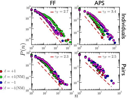
100 101 102 103

10-6

10-4

10-2

100

100 101 102

10-6

10-4

10-2

100

100 101 102 103

10-6

10-4

10-2

100

100 101 102

10-4

10-2

100

n

P

(

n

)

FF

APS

Ind

ivi

dua

ls

Pa

irs

100 101 102 103 104

10-6 10-4 10-2 100

100 101 102 103

10-6 10-4 10-2 100

100 101 102 103

10-6 10-4 10-2 100

100 101 102

10-4 10-2 100

`= +1 `= +1(NM) `= 1 `= 1(NM)

I= 2.7 I= 3.4

P= 2.3 P= 2.5

Figure 6: Probability of finding a number n of consecutive interactions occurring on the same layer`, not interrupted by interactions on the other layer,P`(n), for different data sets considered and for the corresponding data randomized according the null model (NM). Probability distributionP`(n) for aggregated point processes constituted by the interactions of a single individuals (top panels) and a pair of individuals (bottom panels). Power-law decays,P`(n)∼n−γ, with different exponent for pairs,γP, and individuals,γI, are plotted in dashed line. Data shown are, from left to right: RM contact networks, data set

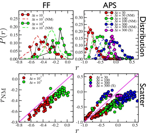
B. Multitasking index of individuals

-0.8 -0.6 -0.4 -0.2 0.0 0.00

0.05 0.10 0.15 0.20

0.25 ∆t = 10

3

∆t = 103 (NM)

∆t = 104

∆t = 104 (NM)

-1.0 -0.5 0.0 0.5 0.00

0.05 0.10 0.15 0.20 0.25 0.30

∆t = 30 ∆t = 30 (NM) ∆t = 100 ∆t = 100 (NM) ∆t = 300 ∆t = 300 (NM) ∆t = 300 (S)

-0.8 -0.6 -0.4 -0.2 0.0 -0.8

-0.6 -0.4 -0.2

0.0 ∆t = 103

∆t = 104

-1.0 -0.5 0.0 0.5 -1.0

-0.5 0.0

0.5 ∆t = 30

∆t = 100 ∆t = 300 ∆t = 300 (S)

FF

APS

Di

stri

buti

on

Sca

tter

P

(

r

)

r

r

r

Figure 7: Comparison of the multitasking index of the original data,r, with the corresponding indexrN Mof data randomized according the null model. Probability distribution of the multitasking index of the original and randomized data,P(r) and P(rN M) (top row), and scatter plot of the multitasking index of the original versus randomized data,rvs.rN M (bottom row), for different time window ∆tand different data sets. In scatter plots, only individuals withrwith a p-value smaller than 0.05 or greater than 0.95 with respect to the null model are plotted. Data shown are, from left to right: RM contact networks, data set FF (∆texpressed in seconds) APS collaboration network (∆texpressed in days). In the APS panels, we also plot the multitasking index of an uncorrelated synthetic network (labeled with S in plots) with the same number of nodes of the APS

C. Influence and predictability between layers

0.0 0.2 0.4 0.6 0.8 1.0 0.0 0.2 0.4 0.6 0.8 1.0

0.0 1.0 2.0 3.0 4.0

0.0 1.0 2.0 3.0 4.0 5.0

0.0 1.0 2.0 3.0 4.0 5.0 6.0 0.0 1.0 2.0 3.0 4.0 5.0 6.0

0.0 1.0 2.0 3.0 4.0 5.0 6.0 7.0 0.0 1.0 2.0 3.0 4.0 5.0 6.0 7.0

FF

APS

M

utua

l

Inf

orma

tio

n

Entr

op

y

H

H

Hu( 1) vsHc(+1! 1)

Hu(+1) vsHc( 1!+1)

I

( 1

!

+1)

I

(+1

!

1)

Figure 8: Scatter plots of the uncorrelated vs conditional entropy of individual i(bottom row),Hiu(`) vs Hic(`→ −`), and mutual information between layers,Ii(+1→ −1) vsIi(−1→+1), for different data sets. Only individuals with a conditional entropy with a p-value smaller than 0.05 with respect to the null model are plotted. Data shown are, from left to right: RM

contact networks, data set FF and APS collaboration network.

III. NULL MODELS OF UNCORRELATED TEMPORAL MULTIPLEX NETWORKS

We consider as a null model of uncorrelated temporal duplex network a multivariate point process formed by two renewal processes32_{, one in each layer`∈ {+1,−1}, with interevent time distributionsφ}

`(τ).

A. Poissonian interevent time distributions

Let us consider in the first place, and as the simplest example, the scenario in which both layers obey a Poisson process39 _{with rateλ}

`, i.e. φ`(τ) = λ`e−τ λ`. Focusing on layer `, assume two consecutive interactions in layer −`

at times t? and t?+τ?, with τ? a random number distributed according toφ−`(τ?). The number nof consecutive,

uninterrupted interactions in layer ` in the interval [t?, t? +τ?] is given by a Poisson distribution32 P`(n|τ?) =

(λ`τ?)ne−λ`τ?/n!. Therefore, the probability of observingn >1 consecutive interactions in layer`is

P`(n) =

Z ∞

0

φ−`(τ?)

P`(n|τ?)

P∞

n0₌₁P`(n0|τ?) dτ?=

λ−` λ`

ζ

n+ 1,λ`+λ−` λ`

∼

_λ

` λ`+λ−`

n

, (4)

in the largen limit, whereζ(x, a) is the Riemann Zeta function. That is, P`(n) shows an exponential decay with a

characteristic number of consecutive events n`,c= 1/ln

_λ

`+λ−`

λ`

. The result in Eq. (4) can be generalized for any interevent time distributions with finite first moment hτi`. In this case, the probability that a random interaction

takes place in layer ` is q` =hτi−_{`</sub>1/(hτi−<sub>`}1+hτi−₋1_`), and the probability of observing n consecutive interactions in

layer`is given by

P`(n) = (1−q`)(q`)n=

hτi−₋1_{`</sub> hτi−<sub>`}1+hτi−₋1_`

hτi−_{`</sub>1 hτi−<sub>`}1+hτi−₋1_`

!n

, (5)

B. Power-law interevent time distribution

Calculations in the Poissonian case are much simplified by the memoryless nature of these processes39_{. In the}

general case of non-Poissonian interevent time distributions, they become more involved, especially in the case of long tailed interevent time distributions, as those found in empirical temporal multiplex networks. Focusing again in layer

`, let us assume two consecutive events in layer−`, at timest?andt?+τ?. The number of eventsnin this interval in

layer` will depend also of the time of the last interaction in this layer, occurring at timet`< t?, i.e. the number of

eventsn depends on the aging timeta =t?−t`. The probability for the number of consecutive interactions in layer `will then be given by

P`(n) =

Z ∞

0

φ−`(τ?)P`(n|ta, τ?)dτ?, (6)

where P`(n|ta, τ?) is the probability of observing n renewal events in layer ` in the interval [t?, t?+τ?], knowing

that the last renewal in ` took place at time t`. Analytic expressions for this function can be obtained in Laplace

space33_{. They are however quite cumbersome, so, for the sake of simplicity, we will consider the non-aged caset}

a = 0,

in which we assume that the last interaction in layer ` happened simultaneously with the first interaction of the interval considered in layer−`,t?=t`. Under this assumption, if we consider power-law forms of the interevent time

distributions, φ`(τ) = α`c`(c`τ+ 1)−1−α`, where c` is some scale parameter, we can approximate33, in the limit of

largen/(c`τ?)α`,

P`(n|0, τ?)∼(c`τ?)−α`e−A(n/τ

α`

? )1/(1−α`)_{, (7)}

whereAis a positive constant, depending on the parameters (c`, α`) of the interevent time distributions. From here,

using Eq. (6), we can obtain, within the non-aging approximation, the scaling form

P`(n)∼n−1−α−`/α`, (8)

IV. NULL MODEL OF A RANDOMIZED TEMPORAL MULTIPLEX NETWORK BY PRESERVING

THE INTEREVENT TIME DISTRIBUTION

In order to evaluate the relevance of the probability distribution of consecutive interactions within the same layer

`,P`(n), and the multitasking index of individualsr, obtained in the empirical networks, we compute this quantities

on a randomized networks. Therefore, we build a null model (NM) of a randomized temporal multiplex network in which we preserve the interevent time distributionψ`(τ) for each layer`, while destroying temporal correlations

between layers. To this end, we define a randomization procedure as follows: For each individual i, we swap all his interactions within the same layer, i.e. we consider the set of pairs{(j1, t1),(j2, t2), . . . ,(jn, tn)}, where a pair (ji, ti)

represents an interaction with individual ji at time ti, we randomize the order of the individuals, {j1, j2, . . . , jn},

and create random pairings with the set of contact timing{t1, t2, . . . , tn}. This procedure ensures that the interevent

time set τ={τ1, . . . , τn−1}, whereτi=ti+1−ti, is kept constant, and so it is the interevent time distributionψ(τ).

At the same time, temporal correlation between layers are washed out. We generate 200 bootstrap replicas for each temporal multiplex by following this procedure, and perform the analysis described in the Sections as done for the original network. We build the distribution of consecutive interactions obtained in the null model of rewired networks,

PN M

` (n), for each layer `, and compare with the original distributionP`(n). For each individual, we calculate his

multitasking coefficient in the rewired network, rN M(∆t), and verify the null hypothesis that this value is only due

to the form of the interevent time distribution. We estimate the probability (p-value) thatrN M(∆t) is as small or as

large as the observed coefficientr(∆t), and reject the null hypothesis if the p-value is smaller than 0.05 or bigger than 0.95. The multitasking index is also computed on a synthetic temporal duplex network, rS(∆t), where each layer

correspond to a temporal network generated independently by using the Non-Poissonian activity driven (NoPAD) model40_{, to ensure the lack of correlation between layers. We choose the same interevent time distributionψ}

`(τ) for

the two layers, power law distributed,ψ(τ) =αc(cτ+ 1)−1−α_{, withα= 1.0 andc= 1.0.}

V. NULL MODEL OF A RANDOMIZED TEMPORAL MULTIPLEX NETWORK BY PRESERVING

THE UNCORRELATED ENTROPY

information is equal to zero, and we estimated the probability (p-value) that the conditional entropy defined in Eq. 2 in the main paper is at least as low as the observed value. We perform a bootstrap resampling for each individual and we reject the null hypothesis if the p-value is smaller than 0.05.

The resampling procedure is performed in a way to keep constant the uncorrelated entropy defined in Eq. 1 in the main paper. To this end, for each individuali we select the set of pairs of consecutive interactions occurring in different layers,{(e`

j1, e −` k1),(e

` j2, e

−`

k2), . . . ,(e

` jn, e

−

kn`)}, where (e

` j, e−

`

k ) is a pair of interactions of individualiwithj in

layer ` and with k in layer −`. To resample these pairs, we randomized the order of the set of second interactions occurring on layer−`,{e−<sub>k</sub>`

1, . . . , e −`

kn}and created random pairings with the set of first interactions occurring on layer`,

{e`

j1, . . . , e

`

jn} thus destroying any temporal correlation between layers. After aggregating the transition probabilities

for the random pairings, we calculated the conditional entropy for the randomized data. We repeated this procedure 200 times and calculate the p-value of each individual.

1 _{M. Jackson,Social and economic networks (Princeton University Press, 2010).} 2

J. L. Moreno,Who shall survive? (Beacon House Inc., Beacon N. Y., 1953), 2nd ed. 3

M. E. J. Newman,Networks: An introduction (Oxford University Press, Oxford, 2010).

4 _{A. Barrat, M. Barth´elemy, and A. Vespignani, Dynamical Processes on Complex Networks (Cambridge University Press,}

Cambridge, 2008). 5

R. Pastor-Satorras, C. Castellano, P. Van Mieghem, and A. Vespignani, Rev. Mod. Phys.87, 925 (2015). 6 _{P. Sen and B. K. Chakrabarti,Sociophysics: An Introduction (Oxford University Press, Oxford (UK), 2013).} 7

J. Leskovec, L. A. Adamic, and B. A. Huberman, ACM Trans. Web1, 5 (2007), ISSN 1559-1131. 8

S. Wasserman and K. Faust,Social Network Analysis: Methods and Applications(Cambridge University Press, Cambridge, 1994).

9 _{L. M. Verbrugge, Social Forces57, 1286 (1979), http://sf.oxfordjournals.org/content/57/4/1286.full.pdf+html, URLhttp:}

//sf.oxfordjournals.org/content/57/4/1286.abstract.

10

S. Boccaletti, G. Bianconi, R. Criado, C. del Genio, J. G´omez-Garde˜nes, M. Romance, I. Sendi˜na-Nadal, Z. Wang, and M. Zanin, Physics Reports544, 1 (2014), ISSN 0370-1573.

11

M. Kivel¨a, A. Arenas, M. Barth´elemy, J. P. Gleeson, Y. Moreno, and M. A. Porter, J. Complex Networks2, 203 (2014). 12

K.-M. Lee, B. Min, and K.-I. Goh, Eur. Phys. J. B88, 48 (2015), ISSN 1434-6028, 1502.03909, URLhttp://link.springer.

com/10.1140/epjb/e2015-50742-1.

13

M. De Domenico, A. Sol´e-Ribalta, S. G´omez, and A. Arenas, Proceedings of the National Academy of Sciences111, 8351 (2014), ISSN 0027-8424, 1306.0519, URLhttp://dx.doi.org/10.1073/pnas.1318469111.

14 _{S. V. Buldyrev, R. Parshani, G. Paul, H. E. Stanley, and S. Havlin, Nature464, 1025 (2010).} 15

O. Yagan, D. Qian, J. Zhang, and D. Cochran, Selected Areas in Communications, IEEE Journal on31, 1038 (2013), ISSN 0733-8716.

16 _{M. Dickison, S. Havlin, and H. E. Stanley, Physical Review E85, 066109 (2012).} 17 _{P. Holme and J. Saram¨aki, Physics Reports519, 97 (2012).}

18

P. Holme, Eur. Phys. J. B88, 234 (2015), ISSN 1434-6028, arXiv:1508.01303v1, URLhttp://link.springer.com/10.1140/

epjb/e2015-60657-4.

19 _{J. G. Oliveira and A.-L. Barabasi, Nature437, 1251 (2005).} 20

J. Stehl´e, N. Voirin, A. Barrat, C. Cattuto, L. Isella, J.-F. Pinton, M. Quaggiotto, W. Van den Broeck, C. R´egis, B. Lina, et al., PLoS ONE6, e23176 (2011).

21 _{M. Kivela, R. Kumar Pan, K. Kaski, J. Kertesz, J. Saramaki, and M. Karsai, J. Stat. Mech. p. P03005 (2012).}

22

L. E. C. Rocha, F. Liljeros, and P. Holme, PLoS Comput Biol7, e1001109 (2011). 23

A. Vazquez, B. R´acz, A. Luk´acs, and A.-L. Barab´asi, Phys. Rev. Lett.98, 158702 (2007).

24 _{R. Parshani, M. Dickison, R. Cohen, H. E. Stanley, and S. Havlin, EPL (Europhysics Letters)90, 38004 (2010).} 25

N. Eagle and A. Pentland, Personal and Ubiquitous Computing10, 255 (2006). 26

Q. Xuan, H. Fang, C. Fu, and V. Filkov, Phys. Rev. E 91, 052813 (2015), URL http://link.aps.org/doi/10.1103/

PhysRevE.91.052813.

27

(????), URLhttp://www.apache.org/. 28

M. E. J. Newman, Proc. Natl. Acad. Sci. USA98, 404 (2001). 29 _{American Physical Society. Data sets for research.(2013), URL}

https://publish.aps.org/datasets.

30 _{M. Starnini, A. Baronchelli, A. Barrat, and R. Pastor-Satorras, Phys. Rev. E85, 056115 (2012).} 31

D. Cox and V. Isham,Point Processes, Chapman & Hall/CRC Monographs on Statistics & Applied Probability (Taylor & Francis, Cambridge, U.K., 1980), ISBN 9780412219108.

32 _{D. R. Cox,Renewal Theory(Methuen, London, 1967).} 33

J. H. P. Schulz, E. Barkai, and R. Metzler, Phys. Rev. X4, 011028 (2014), ISSN 2160-3308. 34

M. C. W. van Rossum, Neural Computation13, 751 (2001).

35 _{B. D. Ripley, Spatial statistics, Wiley series in probability and mathematical statistics (J. Wiley & Sons, Hoboken, NJ,}

36

C. Song, Z. Qu, N. Blumm, and A.-L. Barab´asi, Science327, 1018 (2010), ISSN 0036-8075. 37 _{T. Takaguchi, M. Nakamura, N. Sato, K. Yano, and N. Masuda, Phys. Rev. X1, 011008 (2011).} 38 _{M. Szell, R. Sinatra, G. Petri, S. Thurner, and V. Latora, Sci. Rep.2, 457 (2012).}

39