City, University of London Institutional Repository
Citation
:
Borges, Rafael, Garcez, A. & Lamb, L. C. (2011). Learning and Representing
Temporal Knowledge in Recurrent Networks. IEEE Transactions on Neural Networks,
22(12), pp. 2409-2421. doi: 10.1109/TNN.2011.2170180
This is the accepted version of the paper.
This version of the publication may differ from the final published
version.
Permanent repository link:
http://openaccess.city.ac.uk/11837/
Link to published version
:
http://dx.doi.org/10.1109/TNN.2011.2170180
Copyright and reuse:
City Research Online aims to make research
outputs of City, University of London available to a wider audience.
Copyright and Moral Rights remain with the author(s) and/or copyright
holders. URLs from City Research Online may be freely distributed and
linked to.
City Research Online:
http://openaccess.city.ac.uk/
[email protected]
Learning and Representing Temporal Knowledge in
Recurrent Networks
Rafael V. Borges
†, Artur d’Avila Garcez
†, and Luis C. Lamb
∗,
Member, IEEE
†City University London, London EC1V OHB, United Kingdom [email protected], [email protected] ∗
Federal University of Rio Grande do Sul, Porto Alegre RS, 91501-970, Brazil [email protected]
Abstract—The effective integration of knowledge representa-tion, reasoning and learning in a robust computational model is one of the key challenges of Computer Science and Artificial Intelligence. In particular, temporal knowledge and models have been fundamental in describing the behaviour of Computational Systems. However, knowledge acquisition of correct descriptions of a system’s desired behaviour is a complex task. In this paper, we present a novel neural-computation model capable of representing and learning temporal knowledge in recurrent networks. The model works in integrated fashion. It enables the effective representation of temporal knowledge, the adaptation of temporal models given a set of desirable system properties and effective learning from examples, which in turn can lead to temporal knowledge extraction from the corresponding trained networks. The model is sound, from a theoretical standpoint, but it has also been tested on a case study in the area of model verification and adaptation. The results contained in this paper indicate that model verification and learning can be integrated within the neural computation paradigm, contributing to the development of predictive temporal knowledge-based systems, and offering interpretable results that allow system researchers and engineers to improve their models and specifications. The model has been implemented and is available as part of a neural-symbolic computational toolkit.
Index Terms—Neural-symbolic computation, Integrating do-main knowledge into non-linear models, Temporal knowledge learning, Recurrent neural networks, Model verification, Knowl-edge extraction, Temporal logic reasoning.
I. I
A
LTHOUGH non-linear methods such as neural networks and support vector machines will often provide the most accurate predictions, they are generally unsuitable in domains where validation is required because of their black-box nature. This also complicates maintenance and model integration with existing legacy systems. As a result, the use of neural networks has remained restricted in a number of important application areas. White-box models seek to solve this problem in different ways; neural-symbolic computation [1] offers one way of implementing white-box non-linear prediction. In particular, neural-symbolic systems seek to open the black-box by integrating non-linear modelling with domain knowledge and rule extraction, thus providing insight into the reasoning made by the non-linear prediction. The construction of such principled, integrated models can provide an enriched understanding of the techniques and tools used in Neural Computation, Cognitive Science and Artificial Intelligence (AI). Specifically, temporal models have been fundamental inthese areas. In addition, the problem of knowledge acquisition of sound descriptions of a system’s desired behaviour is a complex and important task in Computer Science [2], [3].
In this paper, we present a neural-computation model ca-pable of (i) representing temporal knowledge operators in recurrent neural networks, (ii) adapting temporal knowledge models given a set of desirable system properties, (iii) training the networks from examples of system behaviours and (iv) extracting a revised temporal knowledge from the trained networks. In the proposed model, symbolic background knowl-edge described by a temporal logic formalism is translated into a recurrent neural network. Modified gradient-descent methods are proposed for learning both from examples and system properties, and the trained network can be translated back into a temporal symbolic representation incorporating the initial knowledge revised by the examples and properties. This process is known as the neural-symbolic cycle [1], [4], [5].
We have implemented the proposed model as part of a neural-symbolic toolkit and performed experiments on bench-mark case studies in the area of model verification and adapta-tion. The results illustrate how model verification and learning can be integrated within a neural computation paradigm, and indicate that the integration of methodologies from symbolic AI and connectionism is relevant for building robust and sound intelligent systems [1], [3], [6].
More specifically, we present a translation algorithm that takes temporal knowledge as input (in the form of temporal logic rules) to produce a NARX network. The fragment of temporal logic used is an extension of the logic used in [14] with a richer language containing both future and past operators. Following the neural-symbolic methodology [1], [15], [16], [17], [18], [19], we then prove that this translation is correct with respect to well-established temporal logic-programming semantics. We then apply a simple pedagogical method [20] for temporal knowledge extraction from trained NARX networks to validate the application. The extraction method is also sufficient for the extraction of trained partial models. This closes the neural-symbolic cycle allowing the encoding of temporal background knowledge into networks, learning from examples and sequence learning by the net-works, and the decoding of the learned models into a re-vised temporal knowledge for understanding and validation of system properties. The application of the neural-symbolic model to the problems of software model verification and adaptation allows the integration of different dimensions of temporal knowledge, including temporal learning and rea-soning about time. The networks are capable of evolving incomplete software specifications from observed examples of system behaviour. Furthermore, information about certain desired properties of the system can be verified against the networks by combining the abstract syntax and the verification capacities of a model checking tool with our learning model. The remainder of the paper is organised as follows. Section II introduces the basics of temporal reasoning, recurrent net-works and neural-symbolic computation. Section III presents a language for temporal knowledge representation by recurrent networks, and show correspondence between the symbolic language and the NARX recurrent networks. Section IV shows how the approach is used for learning from sequences of examples and temporal domain knowledge. In Section V, we apply the approach to a relevant case study showing how the approach can be used for software model verification and adaptation. Finally, we discuss the results, conclude and point out directions for further research.
II. B RW
A. Temporal Reasoning
Temporal logics have been highly successful for represent-ing temporal knowledge about computrepresent-ing systems [8]. For example, Linear Temporal Logics (LTL) and Computation Tree Logics (CTL) are broadly used in Computer Science to analyse models and properties of a system [7], [8]. While LTL uses a linear deterministic approach to the flow of time, CTL allows for the representation of different possible successors for each time point. For simplicity, in this work we focus on the linear approach; more specifically we use a specific logic programming language, taking as reference several works that use temporal logics [8], [21]. We shall consider several past and future temporal operators. The past operators include the representation of the previous time point (denoted by ), always in the past (), sometime in the past (), and the weak and strong variations (Z and S, respectively) of since.
Their complementary future operators are, respectively, the next time point operator (denoted by), always in the future (), sometime in the future (♦), unless (W) and until (U), formally defined in the next section.
Model Checking is one of the most successful applications of temporal logic. It offers a set of automated tools to perform the formal verification of a system’s properties. The system is described as a temporal model so that the satisfiability of a property can be verified automatically. While model checking presents all the advantages of a formal static verification (when compared to the dynamic process of testing), it reduces the need for human intervention [7]. Our experiments include a model checking application as detailed in the sequel. Adding a temporal dimension to the knowledge model imposes some challenges to the task of learning. Symbolic learning systems such as Inductive Logic Programming (ILP) [22] can in principle be adapted for application in temporal domains, but will typically require the use of a correct background knowledge (which may not be possible when dealing, for example, with evolving system specifications). ILP may also turn out to be too brittle for modelling dynamic systems and the task of temporal learning, where a large number of very small adjustments may be required to guarantee robustness, rather than concept-level learning [23].
B. Recurrent Networks
Recurrent networks extend the simple feedforward models by allowing activation propagation to neurons in previous layers, thus adding a loop to the network. As a result, such activation values are considered in future computations of the network. A typical recurrent network used for temporal learning is theElman network[24] which adds neurons in the input layer calledcontext unitsto recurrently receive the output values of hidden neurons. Another way of propagating values through time in neural networks is through delay units. Such units output the result of a function applied to the last values received by the input. The most elementary delay unit outputs the value applied to the input at the previous time point. The
Nonlinear Auto-Regressive eXogenous model (NARX) has a feedforward core with delay units before the input layer, and delayed recurrent links from the output to the input layer. They have been proven equivalent to Turing machines [12].
Definition 1 Let xi(t)denote the value of the i-th input neuron
at time t. Let yj(t)denote the value of the j-th output neuron
at time t. NARX allows the use of xi(t)and yj(t)as input at the
next time points t+1, t+2, etc. If xi is connected to a delay
unit z−1, it will be available at t+1. A chain of such units can get the value shifted through time and available at t+2, etc. It is this variable-size chain that makes NARX convenient for temporal reasoning.
MLP (core) z
z
z
z
Output Input -1
-1
-1
[image:4.612.105.245.52.149.2]-1
Fig. 1. The NARX architecture
the error component at the input is propagated through the recurrent links to the output neurons in order to be processed by the next backpropagation and weight change step.
C. Neural-Symbolic Computation
Recent studies in artificial intelligence and evolutionary psychology have produced a number of cognitive models of reasoning, learning and language that are underpinned by neural computation [26], [27], [28]. In addition, recent efforts in computer science have led to the development of computational models, called neural-symbolic systems, inte-grating learning, reasoning and action [4], [1], [29], [30], including first-order logic systems [31], [32]. Such systems have shown promise in a range of applications, including computational biology, fault diagnosis, fraud prevention [16] and other applications such as, more recently, assessment and training in simulators [33]. The connectionist inductive learning and logic programming (CILP) system [16] is a neural-symbolic system showing a one-to-one correspondence between logic programming and neural networks that are trainable by backpropagation [25].
Definition 2 A logic program is a set of rules of the form A← L1,L2, ...,Ln, where A is known as an atom and Li(1 ≤
i≤n)are called literals. A literal is either an atom (A) or its negation (∼A). A rule like A←L1,L2, ...,Ln states that A is
true if L1and L2and, ...,and Lnare true. When n=0 we have
simply A←, and A is said to be a fact1
The CILP translation from logic programs to neural networks produces single-hidden layer feedforward networks that map each of L1,L2, ...,Ln to input neurons and A to an output
neuron. The networks use a bipolar activation function so that an interval (−1,−Amin] represents truth-value false, interval
[Amin,1) represents truth-valuetrue, and (−Amin,Amin) denotes
unknown. Positive weights are used to represent positive liter-als, while negative weights represent negative literals. Hidden neurons implement a logical and of the input, and output neurons implement a logical or of the hidden neurons. The CILP translation algorithm (described in Fig. 2) sets weights and biases in the network so that the network can be proved equivalent to the original logic program [16]. In other words, the network becomes a computational model for symbolic logic programming. In the algorithm, we have the following parameters:
1As is usual, we consider the ground instances of a (first-order) logic
program and assume it is finite.
k(l) denotes the number of literals in the body of a clauseCl;
µ(l) is the number of clauses with the same head asCl.
Maxkµis the maximum among the values ofk(l) andµ(l), and
among every clauseCl∈ P.
Amin is defined in such a way that
1−Maxkµ
1+Maxkµ <Amin<1. φ(x) is the bipolar sigmoid function 1+2e−βx−1, whereβis the parameter that defines the slope of the function;ψ(x) is a linear function (identity).
W is the weight of the positive connections,−W is the weight of negative connections.W is defined as a value greater than
ln(1+Amin)−ln(1−Amin)
Maxkµ(Amin−1)+Amin+1·
2
β to guarantee equivalence (see [16] for the
proofs). Figure 3 shows a CILP network that represents the
CILP Translation(P)
foreachCl∈Clauses(P)do InsertHiddenNeuron(N,hl); foreachA∈Body(Cl)do
ifinA<Neurons(N)then InsertInputNeuron(N,inA); Activation(inA)←ψ(x); Connect(N,inA,hl,W); end
foreach∼A∈Body(Cl)do ifinA<Neurons(N)then
InsertInputNeuron(N,inA); Activation(inA)←ψ(x); Connect(N,inA,hl,−W); end
ifoutHead(Cl)<Neurons(N)then InsertOut putNeuron(N,outHead(Cl));
Connect(N,hl,outHead(Cl),W);
Bias(hl)← −(1+Amin)(k(l)
−1)
2 W;
Bias(outHead(Cl))← −
(1+Amin)(1−µl)
2 W;
Activation(hl)←φ(x); Activation(outHead(Cl))←φ(x);
end
foreachA∈Atoms(P)do
if(inA∈Neurons(N))∧(outA∈Atoms(N))then Connect(N,outA,inA,1)
end returnN;
[image:4.612.313.566.219.488.2]end
Fig. 2. CILP translation algorithm
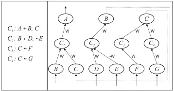
logic program A ← B,C; B ← D,∼ E; C ← F;C ← G. The CILP system uses the translation to add background knowledge (provided in the form of the logic-program rules) to the neural network. This network can be trained by examples in the usual way. The training examples can change or extend the background knowledge. An extraction algorithm then closes the learning cycle, deriving a revised logic program from the trained network. This process of knowledge revision using neural networks and background knowledge is the main
C : A B, C1
C : B D, 2 ~E
C : C F3
C : C G4
C1 C2 C3 C4
A B C
B C D E F G
W W W W
W W -W W W W
[image:4.612.348.527.633.727.2]application of the CILP system.
III. TK RN
A. The Sequential Connectionist Temporal Logic (SCTL)
To allow the representation of temporal knowledge in an integrated reasoning and learning system, we consider the use of a language both simple, to allow the integration with a neural-symbolic engine, and powerful enough to describe sequences of events and the temporal behaviour of systems. Thus, we extend the usual logic programming syntax with the modal operators of linear temporal logic (LTL), as follows.
Definition 3 An expressionαis defined as a temporal formula if and only if one of the following holds:
(i)α=A, where A is a propositional variable;
(ii)α=β,α=β,α=β,α=βSγorα=βZγ(to represent
the past), whereβand γare also temporal formulas;
(iii) α = β, α = β, α = ♦β, α = βUγ or α = βWγ (to
represent thefuture), whereβand γare temporal formulas.
The operators considered above represent the traditional set of LTL operators, where α (known as the yesterday operator) means that α is true at the previous time point, α (known as the tomorrow operator) means that α is true at the next time point,αmeans thatαis always true in the past and♦α
means thatαwill eventually be true in some future point. The
ZandWbinary operators are the weak version of theSandU
operators, i.e. whileαSβrepresents thatαhas been true since the last occurrence ofβ,αZβwill also be true ifαhas always been true, even ifβnever occurred.U(until) andW (unless) are the future operators corresponding to SandZ.
Definition 4 A temporal clause is an expression αi ←
λ1, λ2, ..., λn, whereαis a temporal formula, andλi(1≤i≤n)
are literals. A literal λcan be either a temporal formula (α) or the negation of a formula (∼α). A temporal logic program
Pis a set of temporal clauses.
We will consider that temporal knowledge is defined by a temporal logic program P. In order to define the semantics of the program, we define the operator TP and use the usual fixed-point approach [34]. The semantics ofPis given by an interpretationFt
P, which assigns a truth-value to each temporal formula α at each individual time point t. We consider a sequential approach whereby information about the past Ft−1
P is defined before the current values of Ft
P are calculated. By definition, Ft
P is a least fixed-point of the meaning operator TP (known as the immediate consequence operator).
B. Formalizing the Temporal Language and Semantics
The iTP operator below defines a consequence relation between the body and the head of the clauses, and the semantics of the(previous time) and(next time) operators.
Definition 5 The immediate consequence operator iTP of a
temporal program P is a mapping from interpretations to interpretations of P. The application of iTP over an
inter-pretation IPt at a time point t results in a new interpretation at t (iTP(IPt)) that assigns true to an atom α if any of the
conditions below hold:
(1) α is head of a clause in the form α← λ1, λ2, ..., λn and IPt(λ1∧λ2∧...∧λn)is true.
(2) αis an atom in the formβ, and βis true inFPt−1.
(3) αis true in Ft−1
P .
In order to derive some properties of this consequence opera-tor, we will need sometimes to restrictPto programs that ad-mit a single supported model, so that the consequence operator will provably converge to this unique model. Examples of such programs are acyclic programs, as defined below, although the class of such useful programs is more general. The reader is referred to [34] for more details.
Definition 6 The consequence graph GP of a programPis a
directed graph defined by a different vertex to represent each different temporal expression α in P. If an expressionβ (or
∼ β) is in the body of a clause α ← ..., β, ... then GP will
contain an edge from the vertex representing β to the vertex representing α(the head of the clause). A programPis said to be acyclic if GP is an acyclic graph.
If P is acyclic, the recurrent network representing P will converge in a specific time pointtto a fixed-point that contains all of the logical consequences ofP.
Theorem 7 Given any acyclic temporal program P, iTP
converges to a fixed point iTPν =iTν−1
P with νP given by the
maximum length amongst all of the paths in the graph GP.
Proof: Let G0 denote the set of vertices inGP that are not a target of any edge, i.e. the set of vertices representing expressions not appearing as head of any clause inP. Every expression represented by nodes in G0 will have a constant
value assigned throughout the executions of iTP at t. This value is either given by an input assignment or it is false by default. LetG1denote the set of vertices inGPthat are targets of edges with sources exclusively inG0. For the expressions
represented by the vertices inG1, a single execution ofiTP is sufficient for convergence. This is because the interpretations of the body of these expressions will not change after the first execution. An inductive application of this idea to G2 (i.e.
nodes with edges departing fromG1 andG0only),G3, and so
on, is sufficient to prove that the interpretations will converge for every expression, and that the maximum path withinGP gives the number of executions of iTP that is sufficient to reach such a fixed point.
Recall that we use Ft
P to denote the fixed point of iTP at each time point t. In order to calculateiTP at a time pointt, we assume that νP executions of iTP were performed at the previous time pointt−1. We assume a time flow starting at
t =1 and a virtual time point t =0 where α is true in F0
P only ifαis an expression of the formαor αZγ. Otherwise,
α is false in F0
P. Let us now define the full set of temporal operators under a consequence operator TP. We continue to adopt the sequential approach adopted before.
Definition 8 The immediate consequence operator TP of a
temporal program P is a mapping from interpretations to interpretations of P. The application ofTP over an
true to any atom αwhen one of the following conditions hold (the definitions below follow the intuitive definitions of the past and future operators as discussed informally earlier, including the variations taking into account the current time point):
1) iTP(ItP)(α)is true;
2) α=βand bothFPt−1(β)and IPt(β)are true;
3) α=βand eitherFPt−1(β)or IPt(β)are true;
4) α=βSγand either ItP(γ)is true or bothF
t−1
P (βSγ)and
IPt(β)are true;
5) α=βZγand either IPt(γ)is true or bothF
t−1
P (βZγ)and
IPt(β)are true;
6) IPt(α)is true;
7) α=βandFt−1
P (β)is true; 8) α=♦β,Ft−1
P (♦β)is true andF
t−1
P βis false;
9) There exists some formulaβ such that IPt(βUα) is true and It
P(β)is false; 10) α=βUγ,Ft−1
P (βUγ)is true and I
t
P(γ)is false; 11) There exists some formulaβsuch that It
P(αWβ) is true
and It
P(β)is false; 12) α=βWγ,Ft−1
P (βUγ)is true and I
t
P(γ)is false.
C. Representing SCTL in NARX Networks
To incorporate the above extended semantics into SCTL we make use of a useful symbolic manipulation. More specifically, we extend the original logic programPwith clauses that can represent the different temporal operators through the use of the operator. Basically, we use a recursive definition w.r.t. the prior and present time points. In this way, a formula α
is true at t=1 if αis true att=0. αis true at time points
t >1 if α is true att andα is true att−1. The complete list of definitions is given in the algorithm of Fig. 4. This will allow the representation of any of the temporal operators in the NARX model.
We turn now to showing that the translation obtained from the algorithm of Fig. 4 is logically sound. This result will be needed later to show soundness of the NARX model.
Lemma 9 LetPandP1 be temporal logic programs. LetP1
be the output of the algorithm in Fig. 4 given input P. For every formula α inP,α is true in TP(It) if and only ifα is
also true in iTP1(It).
Proof: The algorithm adds clauses to the program re-specting the semantic definitions of the operators. We can verify this by analysing each case. Take the case of the
S operator. The first clause inserted (βSγ ← γ) represents
exactly the first option in item 5 of Definition 8. Since α represents information about αat time pointt−1, the clause
βSγ←β,(βSγ) represents the second option in the definition ofS. The remaining of the proof is as follows: (→) Assuming that TP(It)(α) is true, we have two possibilities: ifiTP(It)(α) is true then clearly the clauses inserted do not change α’s truth-value and iTP1(It)(α) will be true. If not, a clause will
be inserted by the algorithm, and the interpretation of the conjunction of the literals in the body of this clause will be true; thus iTP1(It)(α) will be true. (←) If TP(It)(α) is false then none of the clauses inserted by the algorithm will change the interpretation ofα, andiTP1(It)(α) will also be false.
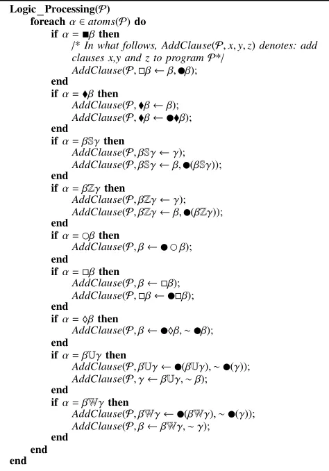
Logic Processing(P) foreachα∈atoms(P)do
ifα=βthen
/*In what follows, AddClause(P,x,y,z)denotes: add clauses x,y and z to programP*/
AddClause(P,β←β,β);
end
ifα=βthen
AddClause(P,β←β);
AddClause(P,β←β);
end
ifα=βSγthen
AddClause(P, βSγ←γ);
AddClause(P, βSγ←β,(βSγ)); end
ifα=βZγthen
AddClause(P, βZγ←γ);
AddClause(P, βZγ←β,(βZγ)); end
ifα=βthen
AddClause(P, β← β);
end
ifα=βthen
AddClause(P, β←β);
AddClause(P,β←β);
end
ifα=♦βthen
AddClause(P, β←♦β,∼β);
end
ifα=βUγthen
AddClause(P, βUγ←(βUγ),∼(γ));
AddClause(P, γ←βUγ,∼β); end
ifα=βWγthen
AddClause(P, βWγ←(βWγ),∼(γ));
AddClause(P, β←βWγ,∼γ); end
[image:6.612.315.552.61.400.2]end end
Fig. 4. Logic processing of different temporal operators
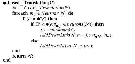
In what follows, we will use the CILP translation to define the feedforward core of the NARX model. We will then make use of the NARX recurrent connections and delay units to implement the temporal operators on top of the feedforward core. As mentioned above, we use a temporal representation based on a sequential approach, where the knowledge about the past is used in the inference of new information about the future. Following this approach, our strategy to represent temporal knowledge is based on the propagation of values through a time flow, from a time pointt−1 to its subsequent time point t. The semantics adopted for our temporal logic programs follows strictly this idea. Our next step is to see how to implement the delayed propagation of information in the neural-network model.
of the network is a key difference between SCTL and CILP, where there are no delays or sequence of inputs. In SCTL, the delay units cater for the representation of value propagations over time. For example, this allows a neuron representing a formulaαto receive as input the value ofαcomputed at the previous time point by the network, and produce the correct output. In the same way, an input neuron representing αcan receive att the value ofαcomputed att−1. In this section, we present an algorithm to translate SCTL into NARX and show that the translation is correct w.r.t. the semantics of the temporal operators.
We have considered different ways of representing SCTL in a neural network. The first idea was to use only (delayed) recurrent links to carry the value of an output neuron rep-resenting a formula α into an input neuron representing α. Whenαappears in the head of a clause, the CILP translation generates an output neuron representing α. Whenαdoes not appear in the head of a clause, CILP will not have α in the output, and, in the temporal case, it would not be possible to linkαtoαand respect the semantics of theoperator. One solution to this is to add clauses of the form α ← α every time a formula α appears in a program P and α is not in the head of any clause in P. In this case, the value of νP is incremented by one due to the insertion of a new clause.
Another approach makes a better use of the available resources of NARX and produces a smaller network. This approach is to use the delay units before the input units to compute the value of α before computing the value ofαin the input. In this case,αdoes not appear in the output because it is not in the head of any clause. In this way, we avoid having to add clauses to the program and produce a smaller network as a result. For each formula of the form nα, we insert the delay units as follows (below, we use the notationoperatornα
to denote n applications of an operator over α, for example, 3αdenotes α):
• If a formulaiαappears as head of a clause inPwhere 0≤i<n, create a recurrent link from the output neuron representingmax(i)αto the input neuron representingnα and setn−max(i) as the number of delay units. • If no formula iα appears as head in P, add n delay
units before the input neuron representing nα (so that this neuron will receive the value ofαat time pointt−n). • If a formula nα appears as head of a clause in P (n > 0), create a recurrent link from the output neuron representing nα to the input neuron representing the formulaiαwithmax(i)<n and setn−i as the number of delay units.
The algorithm of Fig. 5 takes a temporal logic program as input and produces a NARX model. It is an adaptation of the CILP algorithm and it produces networks with an appropriate set-up of the delay units to implement the temporal constraints.
Theorem 10 Given a temporal logic program P, a NARX neural network N can be built such thatN computes TP.
Proof:For the first time pointt=1, given arbitrary initial values for the •α formulas, we have that the computation of TPis the same as in CILP networks, and it converges to a least fixed point [16]. Inductive step: at a time pointt0, eitherN is
-based Translation(P)
N ←CILP T ranslation(P);
foreachinα∈Neurons(N)do if(α=nβ)then
if∃i<n(outiβ∈neurons(N))then j←maximum(i);
AddDelayLink(N,n−j,outjβ,inα);
else
AddDelayInput(N,n,inα);
end returnN;
[image:7.612.317.536.63.168.2]end
Fig. 5. Translation of temporal logic programs into NARX networks
stable withαinFt0
P(I) or the value of αis given as an input. For any formula•nα, if the value of•iα(i<n) is represented
in the output of the network, the recurrent link withn−idelay units will apply the correct value to the input of•nα. If•iαis
not represented in the output for anyi<n, the input value of the neuron•nαis given by the chain of n delay units in the input. This completes the proof.
A corollary of the above theorem is that for acyclic programs, and more generally for any program P admitting a single supported model the corresponding recurrent NARX network N converges to a least fixed point ofTPdenoting the intended meaning ofP. We say thatN computesP; in other words, the neural and symbolic representations become interchangeable. In what follows, we exploit this result to allow learning of symbolic temporal knowledge in NARX networks.
IV. L TKD
Suppose that, in a given application domain, partial sym-bolic knowledge is available in the form of temporal rules (known as a model description). The algorithm of Fig. 5 offers a simple and efficient way of adding knowledge to a NARX model. Suppose, further, that examples are available for training (we call thoseobserved examples). In this section, we describe how the NARX model can be trained with such examples. We also consider a third source of information:
system properties, i.e. properties to be satisfied by the model description.
Let us consider the above three sources of information in the context of an example. In a water pump system (this is our case study to be discussed in more detail in the next section), an engineer seeks to produce a model description of the system so that it can be implemented and formally verified for errors (since it is a safety-critical system). The engineer starts by defining certain rules, for example, at any time, if the engine temperature is too high, the pump should be turned offno more than five time steps later. This is part of the partial model description that can be directly translated into the NARX model by the algorithm of Fig. 5. Producing a sound and complete description is a difficult task, but our engineer might have access to input-output examples that might help (e.g.at time t1 the temperature was registered as too high, at time t2
the pump was turned off, at time t3, the pump was turned on
logs of the current partial model description itself. These are our observed examples to be trained by backpropagation in the NARX model after the partial description has been translated into it. Finally, the engineer may need to verify certain properties (e.g.it must never be the case that the water level is high and the level of methane is high and yet the pump is on), and indeed train the NARX model further to try and satisfy these properties when they have not been verified.
In what follows, the temporal logic programs Pwill form part of the model description. A model description consists, in addition to the temporal program, of a number of input variables and state variables. Input variables are those whose values are set externally to the model, while state variables have their values defined according to the model’s behaviour. In the NARX networks, the state variables are represented by the neurons that are recurrently connected. Given observed examples and system properties, sets of input-output examples will be produced for the training of the NARX network. The resulting network is expected to encode a revised model description, be capable of sequence learning and property verification, and produce a final model description that can satisfy the system properties. The learning process will consist of the application of examples to the network in a supervised way. Each training example will be defined as a vector of input values and desired output values in the usual way. An error between desired and obtained network outputs will be minimised through gradient-descent in a backpropagation-like learning process. Below, we give a general definition that includes the case where information about an output is absent.
Definition 11 Amodel descriptionis a tuple M=hS t,In,Pi, where S t is a set of state variables α, In is a set of input variables β, and Pis a set of temporal clauses of the form α←α1, ..., αn, β1, ..., βm.
Each observed example should assign values to all the input variables and to a subset of the state variables. In other words, the model allows partial observation of state variables. The examples are, thus, defined as follows.
Definition 12 An observed example E at time point t is a tuple Et = hIt,Dt+1i, where the mapping It : In → {−1,1}
assigns values to the input variables and Dt+1 :S t→ {−1,0,1}
makes an assignment of desired values to the state variables at the next time point, where 0denotes that no information is available about the corresponding variable.
As mentioned above, we use gradient-descent on the set of tuples {Et}, 0 ≤ t ≤ n. First, background knowledge P can
be added to the network using the translation algorithm from the previous section. Then, for observed examples, standard backpropagation applies since each tuple relates ti with ti+1.
For each time point t, the usual two-stage computation takes place. In the forward step, the network computes the next state
St+1 given the values of the input vector It and the current
state St (which may be unknown, as defined above). In the
backpropagation step, the error is calculated as the difference between St+1 and Dt+1, and the weights are adjusted in the
usual way [25]. In the case of system properties, the learning above needs to be modified to account for gaps in the sequence
of examples, as detailed below. System properties express the expected behaviour of a system after an entire sequence of inputs and associated states are presented to the system. Formally:
Definition 13 Asystem propertyXis defined by a tupleX= {S0,I,Dn}, where S0 is a initial state, Dn is a desired final
state, and I is a sequence of input variables I0, ...,In−1 with
Sk:S t→ {−1,0,1}and Ik:In→ {−1,0,1}.
Definition 14 Avalue assignmentto the state variables St is
said to correspond to a state condition Skif for everyα∈S t,
St(α) =Sk(α) or Sk(α) =0. The definition is analogous for
input variables.
A property, thus, defines that if the current state of the system at time point t corresponds to S0, the input applied to the
system corresponds to I0, and thereafter each input applied
to the system at time pointt+kcorresponds to Ik until k is
equal to a predefined sizen, then the new state of the system
Sn must correspond to the desired stateDn. When a value of
zero is assigned by a state (or input) condition to a variable
α∈St (or β∈In) then that condition should not impose any
constraint on the value ofα(orβ).
Property learning requires the propagation of errors through the recurrent connections as described in Section II-B. In the forward step, the network computes stateS1 given the values
of the input vector I0 and the current state S0, but also S2
givenI1 andS1 and so on, up toSn. In the backpropagation
step, the error is calculated as the difference between Sn and
Dn and propagated back through the network and its recurrent
connections n times before the weights are updated in batch mode in the usual way.
A. System Implementation
We have implemented the above algorithms as part of a unified neural-symbolic system. The system allows the translation of SCTL knowledge into NARX networks, learning from examples and properties, and knowledge extraction from trained NARX networks (discussed in the sequel). Among the several functionalities, it allows the creation of NARX networks from temporal logic programs, as well as the creation of arbitrary architectures of feedforward and NARX networks without background knowledge. The networks can then be subject to learning, with a functionality for evaluating training and test-set performances using cross-validation. The system allows the combination of different sources of information, notably, learning from observed examples and properties. It can also handle learning from multiple properties. Moreover, it includes a tool for automated pedagogical extraction of revised SCTL knowledge from trained NARX networks, rule simpli-fication and visualization through state-transition diagrams.
When both examples and multiple properties are to be learned simultaneously, the system keeps a record of active properties (initially empty) and an index k for each active property. At each time pointt, if the current state corresponds to the initial state conditionS0of a propertyXthenXbecomes
position Ink of each active property X, eliminating from the
list of active properties all the properties not satisfying this condition. When a property becomes inactive, the assignments to the state variables given by the final state condition Sn
are used to define the desired output values then used as part of the learning process. The above mechanism is also used when no examples, but only properties are available. In this case, the properties provide the desired output of the network and the inputs to be applied at each time step. At each time-point, a property is selected from the list of active properties randomly. When no information is provided about the desired value of a state variableα, the system uses the value obtained by the network as desired value, i.e. Dt+1 = St+1. This
implements a form of expectation maximization. In this way, the error will be null for that neuron and it will not affect the weight correction in the network. Finally, when there is an inconsistency between the values of properties (or between a property and an example), the system adds up the values into a variable sum, and takes Dt+1 = 1 if sum > 0, Dt+1 = −1
if sum < 0 and Dt+1 = 0 otherwise. Other alternatives are
possible here, and might be considered as part of future work. For example, one could assign priorities to properties and rank them in order to mitigate conflicts. The system implementation and the results from our experiments with water pump case study (described below) are available in
http://vega.soi.city.ac.uk/˜abct616/?cont=2
B. Towards Validating the Model Using Knowledge Extraction
Several approaches to knowledge extraction have been proposed in the literature [35], [36], [37], [5]. In our work, extraction is used as a was of validating our model. Below, we sketch the implementation of the extraction tool, which takes a trained NARX network as input and produces temporal logic programs. The implementation is based on pedagogical strate-gies [20], whereby examples are presented to the network, and the obtained outputs are used to define symbolic rules. In pedagogical extraction, one needs to generate a set of examples (input vectors) to be applied to the network. This set must be large enough to offer a good representation of the domain, but not so large that the extraction becomes computationally intractable. Different approaches trying to strike this balance can be found in the literature. In [35], for example, a partial ordering is imposed on the set of input vectors according to the structure of the network so that certain input vectors become preferred over others for querying the network and rule creation. Although not optimized for efficiency, the simple pedagogical approach user here turned out to be sufficient for our purposes of validating the case study, as detailed later.
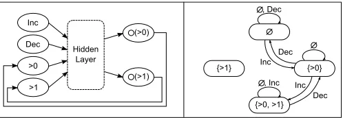
Consider, first, NARX networks where input information is applied directly to the neurons without delay units, and the temporal recurrent links are delayed only by one time point. With these restrictions, at each time point we can associate the input vector I applied to the network to the temporal formulas represented by input neurons. We then run the network once to obtain activation values for the output neurons and, through the recurrent connections, new values for some of the input neurons. Such input neurons that receive
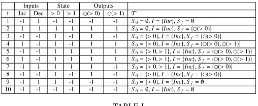
Inc
Dec
>0
>1
(>0)
(>1) Hidden
Layer
{>0} {>1}
{>0, >1} Inc
Dec
Inc Dec , Inc
[image:9.612.315.564.52.138.2], Dec
Fig. 6. Example of extraction procedure
information from the output are known as context units. It is useful to distinguish input units (those associated with input vector I) and context units (the values of which define a new state given I). Our system implementation extracts symbolic knowledge from NARX networks by creating a state transition diagram mapping the state of the context units to a new state given the input, according to the following definition. Notice that the state diagram is created for visualization purposes, each transition corresponding directly to a temporal rule that can be extracted from the network.
Definition 15 A transition T is a tuple nS0,I,Sf,w,count
o
containing asourcestate S0and atargetstate Sf giveninput
I. Variables w and count are auxiliary information represent-ing aweightand the number of occurrences, respectively.
For each time point, a new transitionT is stored: Irepresents the input vector applied to the network,S0contains the values
of the context units andSf contains the values of the output
units. We assign truth-value true (value 1) to positive values inSf and false (value -1) otherwise, but we use the auxiliary
weight w, calculated as a function of the absolute values obtained in the network’s output, to calculate a confidence interval on the assignment of truth-values. After a set of inputs is applied to the network, all the occurrences of transitionT with the sameS0,IandSf are grouped into a single transition
T0, wherewT0
is the sum of the individual weights andcountT0
is the number of transitions grouped. This information is then used to generate a transition diagram that will visually indicate the behaviour of the network.
As an example, consider a simple case where an input (Inc) is used to increment the value of a counter, an input (Dec) is used to decrement this value, and the output identifies if the value is greater than zero. Assume that this counter is capable of counting from 0 to 2, and therefore a state variable is needed to record if the value is greater than 1. Figure 6 shows a network that represents this example on the left hand side, and a state transition diagram extracted from the network on the right hand side. Table I shows a number of extracted state transitions. When grouping the transitions, those in time-points t = 3 and t = 8 will be grouped in a transition T, while the others remain the same (cf. Fig. 6, right hand side). Besides generating the diagrams, our system implementation also represents the extracted knowledge as temporal logic programs. To do so efficiently, the most important transitions are identified with the use of the auxiliary weight andcount
TABLE I
TE E F. 6
Each remaining transitionT0is rewritten as a set of clauses -one clause for each output variable. The body of each clause will contain all the input and state variables either in positive or negative form according to the assignments of values to
S0 andI. The head of each clause will be one of the output
variables: eitherα, ifSf(α)=1, or¬α, ifST 0
f (α)=−1. To
allow a better understanding of the rule set, rules obtained from different transitions can also be simplified. A technique based on Karnaugh maps is used, whereby complementary literals can be removed from the body of rules with otherwise the same body and the same head, e.g.:a←b,canda←b,∼c can be simplified into a single rule a←b.
The extraction method can be extended to deal with more delays in the network. For delay units inserted in the input, the rule containing that input neuron will have a operator for each delay unit in the network. If, for example, literalαis associated with an input neuron with two delay units,2αwill be used in the rule. The same process can be used for extra delays in recurrent links: if α is associated with output neuron out, and this neuron is connected through two delay units to an input neuron inthenα is added to the rule.
V. CS: ISCTL VT
The intended application of SCTL is in model verification and adaptation. The integration of learning and verification has been considered an important research endeavour [10]. We combine the abstract syntax and the verification capacities of a model checking tool [38] with SCTL/NARX as a repre-sentation language and learning system. Model checking tools have three main components: a description languageused to represent the model, aspecification languageused to represent the properties that should be satisfied by the model and the
verification enginethat will perform the actual verification. If the model does not satisfy the given properties, the engine will generate a set of counter-examples, i.e. sequences of events where a violation of the property occurs. Below, we integrate all these different sources of information into the SCTL learning system, and show how an iterative process of learning and verification can be used in the revision of temporal models.
In order to illustrate the different steps of the approach, we consider the pump system testbed used by [11]. The pump system monitors and controls the levels of water in a mine to avoid the risk of overflow. There are three state variables:
CrMeth indicating that the level of methane is critical,
HiWater indicating a high level of water, and PumpOn
indicating that the pump is turned on. In order to turn on and off such indicators, six different input signals are considered:
sC MOn (switch CrMeth on), sC MO f f (switch CrMeth
off), sHiW (switch HiWater on), sLoW (switch HiWater
off), T urnPOn(switch PumpOn on) and T urnPO f f (switch
PumpOn off). Some of the rules of the system are listed below, where e.g. if at any time the critical methane switch is turned on then, at the next time, the level of methane indicator will be at critical (first rule). Similarly, if the level of methane indicator is at critical at time t and it is not the case that the pump switch is turned off then the pump indicator will be on at time t+1 (last rule). Below, ∼stands for (logic programming) negation.
CrMeth←sC MOn
CrMeth←CrMeth,∼sC MO f f
HiWat←sHiW
HiWat←CrMeth,∼sLoW
PumpOn←T urnPOn
PumpOn←CrMeth,∼T urnPO f f
A. The Description Language Used for Verification
Within the logic programming representation, we will con-sider a fragment of SCTL, allowing the representation of the main aspects of a model checking tool [38]. This fragment satisfies all the properties of the original SCTL language w.r.t. its semantics and translation into NARX. In addition, all the programs in this fragment have the property of being acyclic withνP=1. For simplicity, we restrict the types of variables allowed and we assume that the pump system is deterministic (although it should not be too difficult to handle nondetermin-istic problems given our treatment of unobserved states). An input or state variable can be either boolean or scalar (i.e. may assume one value from an enumerated set). From now on, it will be useful having a clear distinction between input and state variables. The following slight variation of our temporal logic programs definition captures this formally.
Definition 16 A temporal logic program description P is a tuple P= nS tP,InP,InitP,CP,GrPo, where S tP is the set of state variables α, InP is the set of input variables β, InitP is the initial state, defined by a mapping from InP ∪S tP
to {true,f alse} and CP is a set of clauses in the form
α ← α1, ..., αn, β1, ..., βm, denoting that α is true at time t
ifα1, ..., αn, β1, ..., βmis true at time t−1. GrP is defined as a
set of elements in2InP ∪2S tP
.
MODULEPumpSystem
IVAR
s :{sCMOn, sCMOff, sHiW, sLoW, , TurnPOff};
VAR
CrMeth :boolean; HiWat :boolean; PumpOn :boolean;
ASSIGN
init(CrMeth) :=FALSE;
init(HiWat) :=FALSE;
init(PumpOn):=FALSE;
next(CrMeth) :=
case
s=sCMOn :TRUE; s=sCMOff:FALSE;
esac;
next(HiWat) :=
case
s=sHiW :TRUE; s=sLoW :FALSE;
esac;
next(PumpOn) :=
case
s=TurnPOn :TRUE; s=TurnPOff:FALSE;
esac;
TABLE II
M PS
B. Learning from Counter-examples and Properties
If all the properties specified are satisfied by the model description, the model checker returns a positive answer and the process can stop. Otherwise, the checker returns what is known as counter-examples. These are traces that show why a property has been violated, as formally defined below. In our case study, these examples will be turned into the training examples used so far to help SCTL learn a new model description. The expectation is that, after a number of iterations, all the properties will eventually be satisfied.
Definition 17 A counter-example X is defined as a tuple
X=nSX0,IX,SXno, where SX0 is the initial state condition, SnX is the final state condition, and IX consists of a sequence of input conditions (I0X, ...,IXn−1). Each condition assigns a boolean value to a subset of variables.
A specific state stis said to match a conditionSXi if, for every variable α with values assigned by SXi , SiX(α) = st(α). The same idea will be used for inputs. Using this idea, counter-examples can produce a large set of sequences to be used for training in SCTL/NARX. Counter-exampleX represents that if the current state of the system at time point t matchesSX0, the applied input matches IX0, and the following inputs at time point t+k match IkX (until k is equal to n), the state of the system must not matchSXn (notice that each counter-example
is a sequence of inputs and states that lead to a violation of a property). In order to train the SCTL/NARX, we negate the final state of Xand use the new sequence ending in∼SXn as
a training example in the usual way.
To exemplify this idea, consider the model description of Table II and a safety property expressed in LTL as
G¬(CrMeth ∧HiWat∧ PumpOn), meaning that the pump should not beonwhen the level of methane is critical and the water is high. Table III shows the counter-example produced by the checker. From the counter-example, we obtain a new
system property X0, such that:
SX00={¬CrMeth,¬HiWat,¬PumpOn},I0X0={sC Mon},I1X0=
{sHiW},I1X0={turnPOn}andSnX0 ={¬PumpOn}, withn=2.
Notice thatX0keeps all the information of the initial state and the sequence of inputs and alters the final state in order to relax the constraint on the variable that regulates the actual state of the pump, in this case. Alternative, more sophisticated methods of generating positive examples from counter-examples exist [39], and may be considered as part of future work. The SCTL/NARX learning process could be greatly facilitated, if, for example, the intervention of an expert was possible at this stage. An expert could identify undesirable states in the middle of a counter-example sequence and propose better positive examples than the above, or reduce the specificity of the counter-example to the right level in one fell swoop by identifying a number of undesired cases in one goal.
t State Input
1 ∅ sC Mon
2 {CrMeth} sHiW
3 {CrMeth,HiWater} turnPon
4 {CrMeth,HiWater,PumpOn}
TABLE III
I -
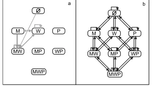
Let us now use the pump system to illustrate the complete iterative process of verification and learning. A sequence of 1000 input-output patterns were used in our experiments. All the state variables were observable and the examples were generated from the model description in Table II. A NARX network was created without any background knowledge and was subject to the successive presentation of these examples. Figure 7 shows a state transition diagram representing the knowledge extracted from the network before (Fig. 7(a)) and after (Fig. 7(b)) the network was trained. In Fig. 7, M representscritical methane(CrMeth), W representshigh water
(HiWat) and P represents that the pump is on (PumpOn). As can be observed in Fig. 7, the NARX starts with a
M
MW MP
MWP WP
W P
O
M
MW MP
MWP WP
W P
O
[image:11.612.356.522.257.318.2]a b
Fig. 7. Transition diagrams: the effects of learning from examples
[image:11.612.362.513.523.609.2]M
MW MP
MWP WP
W P
O
M
MW MP
MWP WP
W P
O
[image:12.612.357.515.49.223.2]a b
Fig. 8. Transition diagrams representing effects of adapting to properties
t State Input
1 ∼CrMeth,∼HighWater∼PumpOn sC Mon
2 {CrMeth,∼HighWater,∼PumpOn} turnPon
3 {CrMeth,∼HighWater,PumpOn} sHiW
4 {CrMeth,HighWater,PumpOn} −
TABLE IV
NC-
Next, let us add to the training the new system property obtained from the counter-example of Table III. In this part of the experiment, we compare the network trained from the examples and the new property with a network created by translating the original rules above and then trained with the new property. Figure 8 shows the transition diagrams extracted in either cases. Notice that in diagram a, the only situation where the pump switches fromo f f toonis when bothCrMeth
and HiWat are false. In diagram b, the only change is in the case where both variables CrMeth and HiWat are true. Considering casebto continue our analysis, one can represent the trained network (with extracted rules) in the form of a new model description. As can be seen from the figure, the new description includes a new condition when turning the pump on. This learned condition does not include the input telling the pump to turn on when the water is high and the methane is at a critical level. It is therefore general enough to deal with different sequences than the one provided in the counter-example. However, the system still does not deal with the case where the pump needs to be turned off because a new input leads to an undesired state. In other words, the new model description still does not satisfy the safety property; this can be verified by a second running of the model checker, as described below.
C. Iterating Verification and Learning
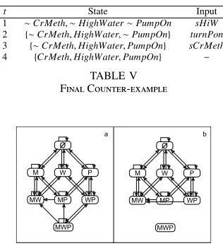
Early work on the integration of verification and learning indicates that a cycle of analysis and revision might converge to a correct specification that satisfies system properties [40]. Our proposal in this paper follows this idea. Therefore, we apply the model checking tool to verify the same property, now on the revised model description. A new counter-example is obtained (Table IV). From the new counter-example, we define a new sequence for training: {} → sC MOn → sHiW
→ T urnPOn → {∼PumpOn}. After this, the diagram shown in Fig. 9(a) was extracted. One can see that the original LTL property is still not satisfied. After verification again, this time we obtain a final counter-example (below). After adapting to this final counter-example, we finally obtain the diagram shown in Fig. 9(b). When applying the model checker to this
t State Input
1 ∼CrMeth,∼HighWater∼PumpOn sHiW
2 {∼CrMeth,HighWater,∼PumpOn} turnPon
3 {∼CrMeth,HighWater,PumpOn} sCrMeth
4 {CrMeth,HighWater,PumpOn} −
TABLE V FC-
M
MW MP
MWP WP
W P
O
M
MW MP
MWP WP
W P
O
[image:12.612.104.245.53.135.2]a b
Fig. 9. Transition diagrams representing effects of iterating properties
new description, the property is finally satisfied (as should be already clear from the diagram).
VI. C FW
We have presented a novel neural-computational model capable of representing and learning temporal knowledge in different domains. The white box methodology presented here is based on solid ideas from AI, Cognitive Science and Neural Computation. The use of a neural-symbolic approach enables the integration of temporal domain knowledge into a non-linear recurrent network model, learning from sequences, counter-examples and system properties, and temporal logic rule extraction from the trained models. The extracted rules can also be visualised through the use of a state diagram tool, and a cycle of learning and verification was implemented through the translation of the model checker into the model. The use of the neural-symbolic methodology enables the use of recurrent networks in domains where traditionally only symbolic methods were used. We seek to promote a robust and effective learning of temporal representations through the use of a connectionist model of computation, yet maintaining sound temporal reasoning and transparency as required by the application. The mains results presented in this paper are: (1) A formal approach that allows the integration of tempo-ral knowledge representation, learning and reasoning into a unified model, making use of a robust connectionist approach for learning, but also providing tools to integrate background information and extracting the learned knowledge. Therefore the proposed methodology overcomes some of the strongest criticisms to neural networks found in literature.
checking tool with several functionalities has led to results clearly useful in relevant application domains [38].
Limitations of the approach include, as discussed and analysed throughout the paper the difficulty in fully-automating the entire process, in particular the process of converting counter-examples into useful training sequences for learning. Extrac-tion is generally perceived as the bottleneck of the neural-symbolic methodology and this is no exception in this paper. Perhaps it is even more so in the case of recurrent networks. Nevertheless, the extraction and validation of partial models has been possible. This opens up a number of research avenues in the area of rule extraction from recurrent networks, which may lead to a range of new applications, as suggested in [39]. In summary, we believe that this paper has described a rich methodology for temporal knowledge representation, learning and verification, shedding new light on predictive temporal models not only from a theoretical standpoint, but also with respect to a potentially large number of applications in Computational Intelligence, Software Engineering, Neural Computation and Cognitive Science.
A
We would like to thank the anonymous referees and Pascal Hitzler for their suggestions which helped improve the pre-sentation of the paper. This work is partly supported by the Brazilian Research Council CNPq.
R
[1] A. S. d’Avila Garcez, L. C. Lamb, and D. M. Gabbay,Neural-Symbolic Cognitive Reasoning, ser. Cognitive Technologies. Springer, 2009. [2] E. A. Feigenbaum, “Some challenges and grand challenges for
compu-tational intelligence,”Journal of ACM, vol. 50, no. 1, pp. 32–40, 2003. [3] L. G. Valiant, “Three problems in computer science,”Journal of ACM,
vol. 50, no. 1, pp. 96–99, 2003.
[4] S. Bader and P. Hitzler, “Dimensions of neural-symbolic integration - a structured survey,” inWe Will Show Them! Essays in Honour of Dov Gabbay, S. Art¨emov, H. Barringer, A. d’Avila Garcez, L. Lamb, and J. Woods, Eds. College Publications, International Federation for Computational Logic, 2005, pp. 167–194.
[5] J. Lehmann, S. Bader, and P. Hitzler, “Extracting reduced logic programs from artificial neural networks,”Applied Intelligence, vol. 32, no. 3, pp. 249–266, 2010.
[6] I. Cloete and J. Zurada, Eds.,Knowledge-Based Neurocomputing. Cam-bridge, MA: MIT Press, 2000.
[7] E. M. Clarke, E. A. Emerson, and J. Sifakis, “Model checking: algorith-mic verification and debugging,”Commun. ACM, vol. 52, no. 11, pp. 74–84, 2009.
[8] M. Fisher, D. Gabbay, and L. Vila, Eds., Handbook of temporal reasoning in artificial intelligence. Elsevier, 2005.
[9] A. Pnueli, “The temporal logic of programs,” inFOCS ’77: 18th IEEE Symp. Found. Comp. Sci. IEEE Computer Society, 1977, pp. 46–67. [10] D. Zhang and J. Tsai, Machine Learning Applications in Software
Engineering. River Edge, NJ: World Scientific, 2005.
[11] D. Alrajeh, J. Kramer, A. Russo, and S. Uchitel, “Learning operational requirements from goal models,” inProc. ICSE, 2009, pp. 265–275. [12] H. Siegelmann, B. Horne, and C. L. Giles, “Computational capabilities
of recurrent NARX neural networks,” University of Maryland at College Park, College Park, MD, Tech. Rep., 1995.
[13] T. Lin, B. Horne, P. Tino, and C. L. Giles, “Learning long-term dependencies in NARX recurrent neural networks,”IEEE Transactions on Neural Networks, vol. 7, no. 6, pp. 1329–1338, 1996.
[14] L. C. Lamb, R. V. Borges, and A. S. d’Avila Garcez, “A connectionist cognitive model for temporal synchronization and learning,” inTwenty Second AAAI Conference on Artificial Intelligence (AAAI07), 2007, pp. 827–832.
[15] R. Sun, “Robust reasoning: integrating rule-based and similarity-based reasoning,”Artificial Intelligence, vol. 75, no. 2, pp. 241–295, 1995.
[16] A. d’Avila Garcez, K. Broda, and D. Gabbay,Neural-Symbolic Learning Systems: Foundations and Applications, ser. Perspectives in Neural Computing. Springer, 2002.
[17] A. d’Avila Garcez and L. Lamb, “A connectionist computational model for epistemic and temporal reasoning,” Neural Computation, vol. 18, no. 7, pp. 1711–1738, 2006.
[18] A. d’Avila Garcez, L. Lamb, and D. Gabbay, “Connectionist compu-tations of intuitionistic reasoning,”Theoretical Computer Science, vol. 358, no. 1, pp. 34–55, 2006.
[19] ——, “Connectionist modal logic: Representing modalities in neural networks,”Theoretical Computer Science, vol. 371, no. 1-2, pp. 34–53, 2007.
[20] R. Andrews, J. Diederich, and A. B. Tickle, “A survey and critique of techniques for extracting rules from trained artificial neural networks,”
Knowledge-based Systems, vol. 8, no. 6, pp. 373–389, 1995.
[21] H.Barringer, M. Fisher, D. Gabbay, G. Gough, and R. Owens, “METATEM: An introduction.” Formal Asp. Comput., vol. 7, no. 5, pp. 533–549, 1995.
[22] S. Muggleton and L. Raedt, “Inductive logic programming: Theory and methods,”J. Logic Programming, vol. 19/20, pp. 629–679, 1994. [23] T. M. Mitchell,Machine Learning. McGraw-Hill, 1997.
[24] J. L. Elman, “Finding structure in time,” Cognitive Science, vol. 14, no. 2, pp. 179–211, 1990.
[25] D. E. Rumelhart, G. E. Hinton, and R. J. Williams, “Learning internal representations by error propagation,” Parallel distributed processing, vol. 1, pp. 318–362, 1986.
[26] S. Pinker, M. A. Nowak, and J. J. Lee, “The logic of indirect speech,”
Proc. Nat. Acad. Sci. U.S.A., vol. 105, no. 3, pp. 833–838, 2008. [27] L. Shastri, “Shruti: A neurally motivated architecture for rapid, scalable
inference,” inPerspectives of Neural-Symbolic Integration, B. Hammer and P. Hitzler, Eds. Springer, 2007, pp. 183–203.
[28] R. Sun, “Theoretical status of computational cognitive modeling,” Cog-nitive Systems Research, vol. 10, no. 2, pp. 124–140, 2009.
[29] L. Valiant, “A neuroidal architecture for cognitive computation,”Journal of the ACM, vol. 47, no. 5, pp. 854–882, 2000.
[30] B. Hammer and P. Hitzler, Eds.,Perspectives of Neural-Symbolic Inte-gration. Springer, 2007.
[31] H. Gust and K.-U. Kuehnberger, “Learning symbolic inferences with neural networks,” in CogSci 2005: XXVII Annual Conference of the Cognitive Science Society, 2005, pp. 875–880.
[32] S. Bader, P. Hitzler, S. Holldobler, and A. Witzel, “A fully connectionist model generator for covered first-order logic programs,” inProceedings of the International Joint Conference on Artificial Intelligence IJCAI-07. Hyderabad, India: AAAI Press, 2007, pp. 666–671.
[33] L. de Penning, A. S. d’Avila Garcez, L. C. Lamb, and J. J. Meyer, “A neural-symbolic cognitive agent for online learning and reasoning,” in
Twenty Second International Joint Conference on Artificial Intelligence (IJCAI-11), Barcelona, July 2011.
[34] P. Hitzler and A. K. Seda, “Characterizations of classes of programs by three-valued operators,” in 5th Intl. Conf. Logic Programming and Non-Monotonic Reasoning LPNMR99. Springer, 1999, pp. 357–37. [35] A. S. d’Avila Garcez, K. Broda, and D. M. Gabbay, “Symbolic
knowledge extraction from trained neural networks: A sound approach,”
Artificial Intelligence, vol. 125, no. 1-2, pp. 155–207, 2001.
[36] R. Setiono, W. Leow, and J. Zurada, “Extraction of rules from artificial neural networks for nonlinear regression,”IEEE Transactions on Neural Networks, vol. 13, no. 3, pp. 564–577, 2002.
[37] R. Setiono, B. Baesens, and C. Mues, “Recursive neural network rule extraction for data with mixed attributes,”IEEE Transactions on Neural Networks, vol. 19, no. 2, pp. 299–307, 2008.
[38] A. Cimatti, E. M. Clarke, F. Giunchiglia, and M. Roveri, “Nusmv: A new symbolic model verifier,” inCAV ’99. Springer, 1999, pp. 495–499. [39] S. Goedertier, D. Martens, J. Vanthienen, and B. Baesens, “Robust process discovery with artificial negative events,”J. Mach. Learn. Res., vol. 10, pp. 1305–1340, 2009.
[40] A. S. d’Avila Garcez, A. Russo, B. Nuseibeh, and J. Kramer, “An analysis-revision cycle to evolve requirements specifications,” in
ACM/IEEE Intl. Conf. Automated Software Engineering (ASE-2001). Los Alamitos, CA: IEEE, 2001, pp. 354–358.
[41] D. Alrajeh, O. Ray, A. Russo, and S. Uchitel, “Using abduction and induction for operational requirements elaboration.”Journal of Applied Logic, vol. 7, no. 3, pp. 275–288, 2009.
[42] D. Peled, M. Y. Vardi, and M. Yannakakis, “Black box checking,”
Rafael V. BorgesRafael Borges received a B.Sc. in Computer Science from the Federal University of Pelotas, Brazil (2004), and M.Sc. in Computer Science from the Federal University of Rio Grande do Sul, Porto Alegre, Brazil (2007). Currently, he is a Ph.D. student at City University London, UK. His research interests include the integration of the symbolic and connectionist paradigms of Artificial Intelligence and formal methods of model specifica-tion and verificaspecifica-tion in Software Engineering.
Artur S. d’Avila GarcezDr. Artur d’Avila Garcez is a Reader in Neural-Symbolic Computation at the School of Informatics, City University London. He holds a Ph.D. in Computer Science (2000) from Im-perial College London. He is a fellow of the British Computer Society. Garcez has an established track record of research in Neural Computing, Artificial Intelligence and Computer Science Logic. He has co-authored two books: Neural-Symbolic Cognitive Reasoning, with Lamb and Gabbay (Springer 2009), and Neural-Symbolic Learning Systems: Founda-tions and ApplicaFounda-tions, with Broda and Gabbay (Springer 2002). His re-search has led to publications in Behavioral and Brain Sciences, Theoretical Computer Science, Neural Computation, Journal of Logic and Computation, Artificial Intelligence and Studia Logica.