City, University of London Institutional Repository
Citation
:
Li, Y. & Sayma, A. I. (2014). Computational fluid dynamics simulations of blade damage effect on the performance of a transonic axial compressor near stall. Proceedings of the Institution of Mechanical Engineers Part C: Journal of Mechanical Engineering Science, doi: 10.1177/0954406214553828This is the accepted version of the paper.
This version of the publication may differ from the final published
version.
Permanent repository link:
http://openaccess.city.ac.uk/7906/Link to published version
:
http://dx.doi.org/10.1177/0954406214553828Copyright and reuse:
City Research Online aims to make research
outputs of City, University of London available to a wider audience.
Copyright and Moral Rights remain with the author(s) and/or copyright
holders. URLs from City Research Online may be freely distributed and
linked to.
City Research Online: http://openaccess.city.ac.uk/ [email protected]
CFD simulations of blade damage effect on the
performance of a transonic axial compressor near stall
Yan-Ling Lia,∗, Abdulnaser Saymab
aThermo-Fluid Mechanics Research Centre, University of Sussex, Brighton, United
Kingdom
bDepartment of Mechanical and Aeronautical Engineering, City University London,
United Kingdom
Abstract
Gas turbine axial compressor blades may encounter damage during service
for various reasons such as damage by debris from casing or foreign objects
impacting the blades, typically near the rotor’s tip. This may lead to
de-terioration of performance and reduction in the surge margin. The damage
breaks the cyclic symmetry of the rotor assembly thus computational fluid
dynamics (CFD) simulations have to be performed using full annulus
com-pressor assembly. Moreover, downstream boundary conditions are unknown
during rotating stall or surge and simulations become difficult.
This paper presents unsteady CFD analyses of compressor performance
with tip curl damage. Computations were performed near the stall boundary.
The primary objectives are to understand the effect of the damage on the
flow behaviour and compressor stability. Computations for the undamaged
rotor assembly were also performed as a reference case. A transonic axial
∗Corresponding author
compressor rotor was used for the time-accurate numerical unsteady flow
simulations, with a variable area nozzle downstream simulating an
experi-mental throttle. Computations were performed at 60% of the rotor design
speed. Two different degrees of damage for one blade and multiple damaged
blades were investigated. Rotating stall characteristics differ including the
number of stall cells, propagation speed and rotating stall cell characteristics.
Contrary to expectations, damaged blades with typical degrees of damage do
not show noticeable effects on the global compressor performance near stall.
Keywords:
Tip curl damage, compressor performance, compressor surge margin,
rotating stall
1. Introduction
Compressor performance plays an important role in gas turbine engines.
It is normally characterised by pressure rise versus mass flow function as
shown in Figure 1. The operating range of the compressor is bounded by the
choke and surge boundaries at a given rotational speed. The surge margin
indicates how close the operating condition of a compressor is to the surge
line. Flow under most of the operating conditions on the map is normally
steady in the rotor’s frame of reference and axisymmetric. When compressors
operate near the surge boundary, mass flow is reduced due to high positive
incidence. When the incidence is beyond the critical value, instability may
it could lead to surge. Surge is a global phenomenon, which is normally
characterised by large mass flow and pressure fluctuations or flow reversal.
Two types of surge are commonly reported in the literature: classic surge and
deep surge. Classic surge normally occurs with large periodic oscillations of
mass flow and pressure while deep surge is a more severe phenomena that
could lead to flow reversal. More details regarding the classification of surge
can be found in Greitzer [1] and de Jager [2].
Figure 1: Part of characteristic map of NASA Rotor 37
Another phenomenon compressors normally encounter before surge is
ro-tating stall, which is the focus of this study. It is commonly associated with
blade vibrations and at extreme conditions can lead to component failure.
Compared to surge, rotating stall is a localised phenomenon to a particular
rotor in which a compressor could operate without failure and may recover.
It consists of one or more stall cells covering one or more blade passages that
shaft speed. The number of stall cells and the propagation speed may vary
at different operating conditions in different compressors, but typically, the
propagation speed is around half of the shaft speed. Rotating stall initiation
mechanisms and characteristics are still the subject of continuous scientific
debate. However, it generally starts with a localised flow perturbation which
causes flow separation on one or more blades due to excessive positive
in-cidence as shown in Figure 2 Iura et al. [3]. The flow separation on the
suction side resulting in the formation of a stall cell which reduces the flow
passing into the passage. Then the blockage diverts flow around the blade so
that the incidence increases on the blade on the right hand side and decreases
on the blade on the left hand side, in the rotating frame of reference. This
leads to the stall cell moving to the passage to the right. This is the start of
propagation of stall cells around the annulus.
Figure 2: Typical stall cells propagation in an axial compressor [3]
There are two well-known routes leading to rotating stall reported by Vo
other starts from a short length-scale or spike inception, distinguished by the
type of initial disturbances in pressure or velocity signals. Modal inception
normally has a small amplitude disturbance with wavelength seen in the
pressure/velocity time histories and requires a large number of revolutions to
develop. Spike inception normally has larger amplitudes with a propagation
speed of 70-80% of the rotor speed. Spike initiated rotating stall is predicted
in this paper.
Although investigations on roating stall drew attention since the 1950’s
and a lot of work in this area has been done so far, surge and/or rotating
stall continue to occur for the reasons such as blade damage, as reported
by Levine [5]. Compressor blades may encounter damage during service for
various reasons such as loose casing liner, Foreign Object Damage (FOD) or
ice formation at the intake. FOD from other sources, such as tire fragments,
injection of bird (bird strike) and runaway debris or animals, may also be
en-countered. This may results in deterioration of the compressor performance
and in extreme conditions, may cause compressor instability. During the
de-sign process, it is important to be able to predict the aerodynamic behaviour
of the compressor in such events to enable the design of robust blades capable
of coping with these events.
A literature search showed that the aerodynamic effects for blade-damaged
compressors have been overlooked. Most of the available material is about
fan blades damaged by bird strike. A 3D simulation of a bird-damaged
was investigated using two damaged blades with different degrees of
dam-age. It was found that flutter stability was reduced and stall was observed
at higher mass flow compared to the undamaged fan.
Another investigation by Frischbier et al. [7] using advanced numerical
methods was reported on bird ingestion in a multistage turbofan. However,
the results showed that the model could not correctly predict the fluid mass
going into the low pressure compressor. Recent studies using the commercial
code ANSYS/LS-DYNA by Meguid et al. [8] and Guan et al. [9] focused
on analysis of structural deformation of fan blades caused by bird strike and
no aerodynamic studies were attempted.
A study of the performance, forced response and surge caused by
ice-damaged blades in Intermediate Pressure (IP) compressor assemblies was
reported by Dhandapani et al. [10]. Results showed that the surge margin
was reduced by increasing the number of damaged blades and the severity of
performance degradation depended on both the number of damaged blades
and their distribution around the annulus.
An aerodynamics study of the effect of bird strike using NASA Rotor 67
was reported by Bohari et al. [11] using CFD. Two damaged assemblies
were simulated at different rotational speeds. It was found that the surge
margin deteriorated at higher rotational speeds and stall was observed before
reaching the working line for both assemblies.
The main objective of this paper is to investigate flow characteristics of
of blade damage on their performance.
2. Description of the compressor
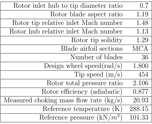
A transonic axial compressor, NASA Rotor 37, was chosen for this study
because of the availability of geometry and experimental data in the public
domain that can be used for numerical model validation. The rotor was
designed as the inlet rotor for a core compressor of an aircraft engine at
NASA Lewis Research Centre in the late 1970 ’s. The rotor has 36
multiple-circular-arc (MCA) blades, a tip speed of 454.14 m/s and a design pressure
ratio of 2.106 at the mass flow rate of 20.19 kg/s with an isentropic efficiency
of 87.7%. The inlet relative Mach number is 1.13 at the hub and 1.48 at the
tip at the design speed of 17,188.7 rpm. The rotor blade has a hub-tip ratio
of 0.7, an aspect ratio of 1.19, and tip solidity of 1.288. The tip clearance
at design speed is 0.356 mm. The main specifications of the compressor are
listed in Table 1 [12].
3. Numerical methodology
3.1. The 3D flow solver
The CFD code used in this investigation is an in-house code, SURF, which
is an implicit time accurate 3D compressible solver based on the methodology
developed by Sayma et al. [13]. It uses an edge-based data structure for
Reynolds-Rotor inlet hub to tip diameter ratio 0.7 Rotor blade aspect ratio 1.19 Rotor tip relative inlet Mach number 1.48 Rotor hub relative inlet Mach number 1.13 Rotor tip solidity 1.29 Blade airfoil sections MCA Number of blades 36 Design wheel speed(rad/s) 1,800 Tip speed (m/s) 454 Rotor total pressure ratio 2.106 Rotor efficiency (adiabatic) 0.877 Measured choking mass flow rate (kg/s) 20.93 Reference temperature (K) 288.15 Reference pressure (kN/m2) 101.33
Table 1: Specifications of Rotor 37
Averaged Navier-Stokes Equations. The Spalart and Allmaras one-equation
turbulence model was used in this investigation.
A mixture of second- and fourth-order matrix artificial dissipation is
ap-plied to stabilise the central difference scheme. For unsteady flow simulations,
dual time stepping is applied with an outer Newton iteration procedure where
time steps are dictated by the physical constraints and fixed throughout the
solution domain. Within the Newton iterations, the solution is advanced
to convergence using the traditional acceleration techniques associated with
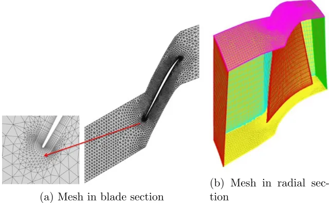
steady state flow solutions [14]. The mesh generation tool provides a
semi-unstructured mesh combining the advantages of structured and semi-unstructured
meshes. A typical mesh used for the rotor is shown in Figure 3. Tip
the casing, which is meshed allowing the flow to pass over the tip. The tip
clearance used in this paper is the same as the one obtained from the
ex-periment at 60% of design speed [15]. Because the flow equations are solved
in a rotating frame of reference, the grid points on the casing are given zero
rotational speed. Hence, it is inherently assumed that a given blade sees the
same mesh points on the casing all the time.
(a) Mesh in blade section
[image:10.612.144.464.278.476.2](b) Mesh in radial sec-tion
Figure 3: Typical mesh used for Rotor 37
3.2. Computational geometry and solution domain
The method used to initiate stall involved gradually throttling the
op-erating point up to the stability limit using steady state simulations. Then
unsteady computations started from solutions obtained from the steady state
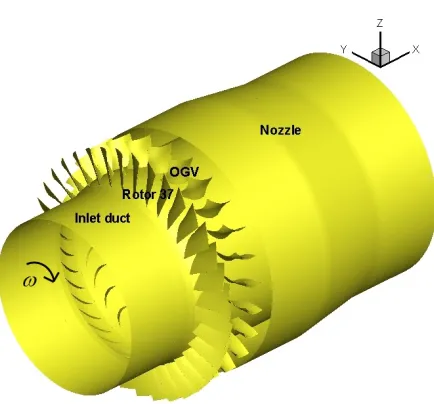
simulations. The domain for steady state computations is shown in Figure 4.
OGV was used to remove the flow swirl downstream of the rotor. Mixing
planes were used between blade rows for the steady state simulations. Since
the axisymmetry of the flow will be broken by rotating stall, it is desirable
to be simulated with a full annulus model. The assembly used in unsteady
computations consists of the same components used in the steady state
anal-ysis, but in full annulus fashion which is shown in Figure 5. Sliding planes
were used at the interfaces of the blade rows instead. Most of the unsteady
simulations were performed by introducing damaged blades into the rotor
as-sembly. The corresponding computational domain contains about 10 million
grid points.
Figure 4: Model for steady state computation
A major difficulty in rotating stall simulations is to specify the
down-stream boundary conditions when there are fluctuations in mass flow and
pressure rise. In this investigation, a methodology reported by Vahdati et
al. [16] using a choked nozzle to control downstream flow boundary
condi-tions was used. The inlet boundary is located at about three chord lengths
upstream of the rotor blade. At the inlet, ambient conditions were assumed
and uniform total pressure and temperature were applied. The nozzle has a
Figure 5: Representing model for unsteady time accurate simulations
Figure 4. Different performance points on the compressor characteristic map
can be achieved by adjusting the size of the downstream nozzle with a
con-stant back pressure. If fixed static pressure profile is provided downstream
of the compressor, the flow is stable under most of the operating conditions.
However, numerical difficulties could be encountered when the compressor
is approaching stall where the downstream boundary conditions are neither
known nor fixed. Therefore, this approach could provide better boundary
condition for rotating stall studies than prescribed pressure profiles. More
4. Model validation
4.1. Grid independence study
It could take a large number ofcompressor revolutions for rotating stall
computations, requiring extensive computational resources. Hence it is
im-portant to strike a balance between grid refinement and the required accuracy
of the solutions, so that fundamental flow features pertinent to rotating stall
are not significantly affected by the grid quality. An extensive investigation
was carried out during this study to choose a suitable grid quality for the
code validation and unsteady computations. Although the primary purpose
of this analysis is to perform unsteady computations, it was only practical to
conduct a grid independence study using steady state single passage analysis
within limited time scale and available computing resources. Only the main
comparisons are presented here, as it is not the main objective of this paper.
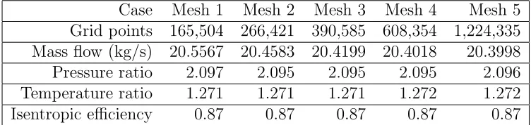
The grid independence study was investigated at the design speed for
a point close to peak efficiency. Five grids of increased refinement in all
directions were used. The number of grid points and a summary of the
resulting solutions are shown in Table 2. As seen in the table, the main
flow parameters changed very little when the grid was refined gradually.
The maximum difference was less than 1%. To examine the flow in detail,
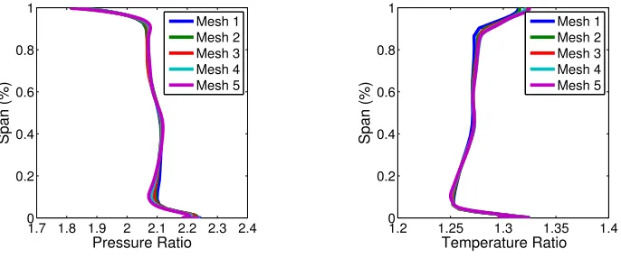
a comparison of pressure profiles at 95% span is shown in Figure 6 and
comparisons of radial distributions of the circumferentially averaged pressure
ratio and temperature ratio are shown in Figure 7. Results show that there
differences mainly around the shock and close to hub and tip in the radial
profiles. Close examinations of the differences show that they decrease as
the grid is refined. Solution on mesh 1 shows the largest difference in most
aspects. However the maximum difference in the pressure rise is much less
than 1%. Mesh 1 and mesh 5 are also investigated at the near stall condition.
The results show that both meshes can capture similar flow pattern and mesh
1 can also capture the key features of the flow near stall. Therefore as limited
by the computational costs, it was decided to use mesh 1 for the unsteady
simulations, but the steady state code validation results presented in the next
subsection were performed on mesh 3.
Case Mesh 1 Mesh 2 Mesh 3 Mesh 4 Mesh 5
Grid points 165,504 266,421 390,585 608,354 1,224,335 Mass flow (kg/s) 20.5567 20.4583 20.4199 20.4018 20.3998
Pressure ratio 2.097 2.095 2.095 2.095 2.096
Temperature ratio 1.271 1.271 1.271 1.272 1.272
[image:14.612.117.493.369.458.2]Isentropic efficiency 0.87 0.87 0.87 0.87 0.87
Table 2: Overall performance comparison for five different grids
4.2. Model validation
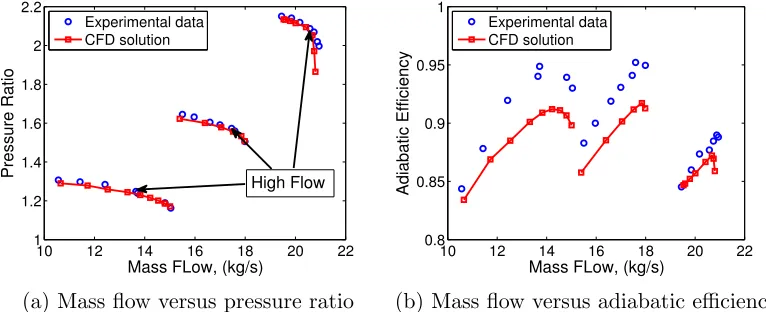
This subsection presents comparisons between experimental data [15] and
CFD simulations. Comparisons of compressor characteristic map at three
different rotational speeds are shown in Figure 8. It can be seen that CFD
solutions have a good agreement with the experimental data for the pressure
ex-0 0.2 0.4 0.6 0.8 1 0 50 100 150 200 250 300 350
Positions on the blade
Norm alised Pressure Mesh 1 Mesh 2 Mesh 3 Mesh 4 Mesh 5
0.4 0.5 0.6 0.7 0.8
60 80 100 120 140 160 180 200
Positions on the blade
[image:15.612.210.386.129.414.2]Norm alised Pressure Mesh 1 Mesh 2 Mesh 3 Mesh 4 Mesh 5
Figure 6: Pressure profile comparison at 95% span
1.7 1.8 1.9 2 2.1 2.2 2.3 2.4 0 0.2 0.4 0.6 0.8 1 Pressure Ratio Span (%) Mesh 1 Mesh 2 Mesh 3 Mesh 4 Mesh 5
1.2 1.25 1.3 1.35 1.4
0 0.2 0.4 0.6 0.8 1 Temperature Ratio Span (%) Mesh 1 Mesh 2 Mesh 3 Mesh 4 Mesh 5
[image:15.612.133.476.455.598.2]plained firstly by referring to Denton [12]. Measurements do not capture
accurately the high loss regions boundary layer due to limitations of the
in-strumentation, which also explains why the pressure ratio matching is much
less affected. Secondly nominal uniform tip clearance values were used for
the three speeds in this study, which are likely to have differences from those
prevailing during the experiment. In addition, CFD predictions may be
af-fected by the use of wall functions and one-equation turbulence model. A
combination of these factors may have contributed to the differences observed
in efficiency.
10 12 14 16 18 20 22
1 1.2 1.4 1.6 1.8 2 2.2
Mass FLow, (kg/s)
Pressure Ratio
Experimental data CFD solution
High Flow
(a) Mass flow versus pressure ratio
10 12 14 16 18 20 22
0.8 0.85 0.9 0.95 1
Mass FLow, (kg/s)
Adiabatic Efficiency
Experimental data CFD solution
[image:16.612.114.497.351.507.2](b) Mass flow versus adiabatic efficiency
Figure 8: Compressor map comparisons (Right to left: design speed, 80% speed and 60% speed)
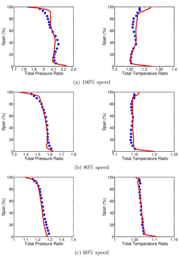
Total pressure ratio and temperature ratio distributions in the spanwise
direction for the three speeds are shown in Figure 9. The solutions from
CFD were circumferentially averaged. Those distributions were obtained at
high flow operating conditions, which were marked in the pressure ratio map
It can also be seen that the code is capable of predicting a typical pressure
deficit at the tip and hub.
These general and detailed agreements between the steady-state solution
and experimental data gave confidence in the ability of the code for
perform-ing accurate predictions for the present study. Since there was no unsteady
experimental data available, further validations using this case were not
pos-sible. However, the methodology was previously validated for unsteady
sim-ulations (See reference [18]).
5. Results and discussion for unsteady simulations
5.1. Unsteady simulation away from stall condition
All unsteady simulations were performed at 60% of the design speed. The
main reason for the choice of this speed is that rotating stall is typically
ob-served at compressor part speed. Before considering the unsteady simulation
of rotating stall, it would be useful to look at the flow field and its behaviour
when operating away from surge line. To capture the unsteady flow
charac-teristics, eight sets of numerical sensors were located in the stationary frame,
positioned about 76% of chord length upstream of leading edge of the rotor.
They were placed 45 degrees apart along the circumferential direction. The
numerical sensors used for all unsteady cases were located at same locations.
8 numerical sensors at different circumferential positions on the casing will
be noted as n1, n2, ..., n8, respectively.
1.7 1.8 1.9 2 2.1 2.2 2.3 0 20 40 60 80 100
Total Pressure Ratio
Span (%)
1.2 1.25 1.3 1.35 1.4 0 20 40 60 80 100
Total Temperature Ratio
Span (%)
(a) 100% speed
1.3 1.4 1.5 1.6 1.7 1.8
0 20 40 60 80 100
Total Pressure Ratio
Span (%)
1.1 1.15 1.2 1.25
0 20 40 60 80 100
Total Temperature Ratio
Span (%)
(b) 80% speed
1 1.1 1.2 1.3 1.4 1.5
0 20 40 60 80 100
Total Pressure Ratio
Span (%)
1 1.05 1.1 1.15
0 20 40 60 80 100
Total Temperature Ratio
Span (%)
[image:18.612.126.476.130.635.2](c) 60% speed
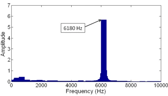
was the only fluctuation observed which shows the periodicity in one rotor
rotation. There are 36 spikes which indicate 36 rotor blades passing the
same sensor in one rotor revolution. In Figure 11, the dominant frequency
is the blade-passing frequency (BPF). The time averaged values of the main
flow parameters from the solution of this case were also compared with the
steady state results. The maximum difference was less than 0.2%. This
also provided confidence to perform the unsteady simulation at near stall
[image:19.612.152.459.320.498.2]condition.
Figure 10: Unsteady static pressure time history at the inlet of rotor without rotating stall
5.2. Unsteady calculations near stall
For the damaged blade study, the investigation was carried out on
as-semblies with different degrees of one damaged blade and multiple damaged
Figure 11: Fourier transform components from one of the numerical sensors on the casing
and flow behaviour when the compressor was operating near stall
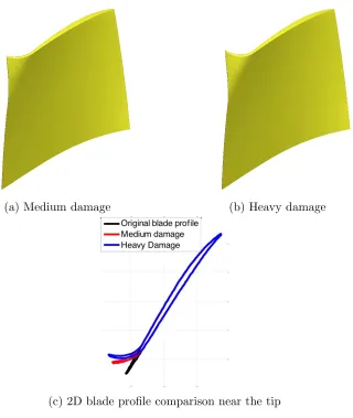
bound-ary. Two different degrees of damaged blades were used as shown in Figure
12. Each damage starts at the leading edge to 20% of chord on the tip and
from 70% span increasing its spanwise extent linearly up to the tip forming
a typical tip curl damage.
Before considering blade damage effect, it is useful to examine the flow
be-haviour and rotating stall characteristics for a case without damaged blades.
It is important to identify a methodology to initiate rotating stall without
excessive computational time. It is well known that in actual geometries
there are small manufacturing tolerances which are believed to contribute to
the onset of rotating stall at specific locations in an assembly.
Computa-tional domains resulting from repeating a single passage mesh are, however,
perfectly symmetric. Previous numerical simulations on those geometries,
(a) Medium damage (b) Heavy damage
[image:21.612.156.476.123.502.2](c) 2D blade profile comparison near the tip
Figure 12: Curl damage at leading edge
are possible. It is likely that accumulated round off errors eventually lead
to some differences among passages leading to the onset of stall at specific
locations. However, that requires the simulation of many rotor revolutions
before the onset of rotating stall happens. It was also found that introducing
small asymmetry of the same order of manufacturing tolerances could lead
significant computer time savings. Therefore, all blades in the computational
domain were randomly staggered between −0.2o and 0.2o to create the
re-quired asymmetry. As reported by Vahdati et al. [19], a larger variation of
stagger pattern was used and it was verified that the results were not affected
regardless of the pattern used.
One operating point (rotor speed: 10313.2 rpm, mass flow: 10.09 kg/s)
was chosen for all unsteady simulations. This point was the near stall point
obtained from steady state simulations which was used as an initial solution
for the unsteady simulation. The unsteady simulation of one rotor revolution
requires about 25 hours using 32, 2.5 GHz Intel Xeon cores. 1350 time steps
per rotor rotation were used for all unsteady simulations reported in this
paper. The unsteady simulation without damaged blades will be discussed
first.
5.2.1. Rotating stall for undamaged assembly
The overall compressor performance during rotating stall for this case is
shown together with the steady state solution in Figure 13. The unsteady
mass flow rate was obtained in the last 10 revolutions. The time averaged
mass flow rate with rotating stall was similar to the near stall point from the
steady state solution but the pressure ratio decreased by approximately 1%.
Figure 14 shows a comparison of the circumferentially averaged axial velocity
profile downstream of the rotor. It can be seen that from about 75% span
that obtained from the steady state solution with no stalled cells. Further
investigation of the detailed flow behaviour allows explaining this. Figure 15
shows Mach number contour comparison at 75% span. It can be seen that
downstream the unstalled passages, the Mach number is higher than that in
the steady simulations due to the low or negative incidence. This indicates
higher mass flow through unstalled passages in the upper part of the passage,
which appears to compensate for the mass deficit in the stalled regions and
the lower part of the passage.
9 10 11 12 13 14 15 16
1.1 1.15 1.2 1.25 1.3
Mass Flow (kg/s)
Pressure Ratio
Steady state solution
[image:23.612.190.402.331.496.2]Unsteady solution without damage
Figure 13: Compressor performance during rotating stall with steady state solutions
5.3. Unsteady calculations near stall
As seen in the full time history from numerical sensors in Figure 16a, after
the initial numerical transient, three different types of spikes can be observed
which indicate three different patterns of stall cells. Rotating stall started
20 40 60 80 100 120 140 160 0
20 40 60 80 100
Axial velocity (m/s)
Span (%)
[image:24.612.201.404.132.251.2]CFD solution for steady state case CFD solution for the undamaged case
Figure 14: Circumferentially averaged axial velocity profile comparison downstream the rotor
(a) Steady state (b) Undamaged case
Figure 15: Mach number contour comparison at 75% span of the rotor
regular pattern was formed at around the 40th revolution with 6 stall cells.
It can be seen that 5 spikes representing 5 rotating stall cells passed the same
sensor in Figure 16b in one engine revolution. Therefore, the propagation
speed of rotating stall cells could be worked out which was 83% of rotor
speed. This information could also be worked out from Figure 17. Three
[image:24.612.117.495.300.491.2]harmonic.
(a) Full time history
[image:25.612.150.456.144.546.2](b) Time history in one rotor revolution
Figure 16: Unsteady static pressure time history from numerical sensors on the casing for the undamaged assembly
For the flow behaviour during rotating stall, the instantaneous negative
axial velocity near the tip of the rotor is shown in Figure 18. It was obtained
Figure 17: Fourier transform components of numerical sensor 7 on the casing
with similar size and approximately equally spaced. Each of them covered
about 60% of the axial domain in the rotor. Rotating stall for this rotor at
design speed was investigated using multi-passage model [20]. For that case,
rotating stall predicted also has 6 stall cells with a propagation speed of 80%
of the rotor speed based on the available data. Stall cells covered about 40%
span of rotor blades and about 4 passages in the circumferential direction.
The spanwise extent of rotating stall is larger than the present study and
could be caused by the interaction between shock waves, boundary layer and
tip clearance flow at design speed while present predictions are performed
at 60% of the design speed. In addition, their simulations were performed
over two engine revolutions only and the solution could have developed to
a different pattern if the simulations were continued beyond that. Figure
19 shows the negative axial velocity on an axial cut in the rotor at the
length downstream from the leading edge at the hub. It also shows stall
cells equally spaced in the circumferential direction and covered about 17%
in radial span. This shows that stall cells are found only near the tip region.
That is a typical behaviour of spike type rotating stall as reported by Day
[21] which shows that stall cells tend to be confined to the tip region of the
rotor suggesting that tip clearance flow is mostly responsible for its inception.
Spike type disturbances have also been experimentally measured to have a
[image:27.612.222.394.326.484.2]circumferential extent of two to three blade passages ([21], [22], [23]).
Figure 18: Instantaneous negative axial velocity near the tip of the rotor
Figure 20 shows 3D streamlines contoured by the negative axial velocity.
The inflow comes from the leading edge of one blade, and the back flow
was reversed at the trailing edge of the neighbouring blade and going into
the passage. It meets the tip clearance flow and the vortex of the stall cell.
The interface between the streamwise inflow and with tip clearance flow is
Figure 19: Instantaneous negative axial velocity on an axial cut plane
of the flow features for the spike initiated rotating stall proposed by Vo et
al [3]. Inside the stall cell the blocked flow diverts the oncoming flow to
the neighbouring area. Outside the stall cell, flow is passing the passages
smoothly without blockage. Stall cell also formed a radial vortex attached to
the blade and the casing. The concept of radial vortex was proposed by Inoue
et al. [24] and also recently confirmed by Weichert et al. [25] and Pullan
et al. [26]. The similarity predicted in this study is due to the design of
this rotor, some blades encounter higher incidence beyond the critical value
near the tip region which leads to separations from the suction side. The
stalled region constitutes a radial vortex attached to the suction side and the
casing. As shown in Figure 20 in the rotor reference frame, when the cell is
propagating in the anti-clockwise direction, the vortex leaves the suction side
of one blade and moves towards the pressure side of the next blade, which
pressure building up which forms the spike in the unsteady pressure signal
time history. This is different from the stall pattern found by Pullan et al.
[26], who predicted a radial vortex starting from the blade‘s leading edge at
the suction side which could be due to the different compressor blade design
used in their analysis where the blades have lower hub to tip ratio and thus
[image:29.612.207.402.270.412.2]rotor blades have much less twist near the tip than Rotor 37.
Figure 20: 3D stream trace inside the stall cell
5.3.1. Rotating stall with one damaged blade
In this subsection the comparison of one damaged blade with different
degrees of damage is discussed. The case with one medium damaged blade
and one heavy damaged blade will be noted as Damaged Case 1 and
Dam-aged Case 2 respectively. A comparison of compressor performance is shown
in Figure 21. For Damaged Case 1, the overall compressor performance
was very similar for the mass flow but the pressure ratio decreased slightly
compared to the undamaged case, which could be caused by rotating stall
slightly larger variation for mass flow and pressure ratio than Damaged Case
1. However, both cases do not have significant influence on the overall
com-pressor performance. The reason for that is the same as for the undamaged
case, the results are similar as shown in Figures 14 and 15. Therefore, they
are not shown here to avoid repetition.
9 10 11 12 13 14 15 16
1.1 1.15 1.2 1.25 1.3
Mass Flow (kg/s)
Pressure
Ratio
Steady state solution Solution without damage
Solution with one medium damaged blade
9.95 10 10.05 10.1
1.27 1.275 1.28 1.285 1.29
Mass Flow (kg/s)
Pressure
Ratio
Steady state solution Solution without damage
Solution with one medium damaged blade
9 10 11 12 13 14 15 16
1.1 1.15 1.2 1.25 1.3
Mass Flow (kg/s)
Pressure
Rat
io
Steady state solution
Solution with one medium damaged blade Solution with one heavy damaged blade
9.95 10 10.05 10.1
1.27 1.275 1.28 1.285 1.29
Mass Flow (kg/s)
Pressure
Rat
io
Steady state solution
[image:30.612.150.452.258.483.2]Solution with one medium damaged blade Solution with one heavy damaged blade
Figure 21: Compressor performance during rotating stall with one damaged blade
It was observed that stall cells started from the damaged blade and
ro-tated in the opposite direction to rotor rotation seen in the relative frame. For
Damaged Case 1 in Figure 22a, after the initial numerical transit, rotating
stall started after 2 revolutions. Then the transition process of 28 revolutions
took place untill a clear pattern was established after the 30th revolution.
of rotating stall. It can be seen from Figure 23a that when increasing the
damage, it takes longer for the flow to settle. In Figures 22b and 23b, it can
be seen that 5 and 6 cells passed the same sensors in that time period for
Damaged Case 1 and Damaged Case 2 respectively. There are small kinks
at the beginning of some of the spikes for both cases with damage, circled
on the plot. That could be the effect that the cell just passed the damaged
blade. Compared to the undamaged case, the rotating stall characteristic is
the same for Damaged Case 1. For the Damaged Case 2, there are 7 rotating
stall cells instead. The propagation speed of rotating cells is very similar to
the other two unsteady cases.
Figure 24 shows the instantaneous negative velocity near the tip. For both
cases with damage, 6 and 7 rotating cells could be observed respectively at
the same time with similar size, shape and approximately equally spaced.
Compared with the undamaged case, the difference is that a non-rotating
stall cell covered the neighbouring region around the damaged blade all the
time after rotating stall started. It is caused by the presence of the damage,
which always diverts the flow. When a rotating stall cell passes through the
damaged blade passage, it merges with the non-rotating cell. After it passes
by, the non-rotating cell recovers to its original state. That could be seen
clearly in the animation. The extent of stall cells in the radial direction can
be seen in Figure 25, which shows the negative axial velocity on an axial
cut plane at 40% chord downstream from the leading edge at the hub. For
(a) Full time history for Damaged Case 1
[image:32.612.170.438.125.420.2](b) Time history in one revolution for Damaged Case 1
Figure 22: Unsteady static pressure signal time history from numerical sensors on the casing for Damaged Case 1
case. The non-rotating stall cell is smaller in the radial direction covering
about 11% of the blade span. For Damaged Case 2, the rotating cells covered
from about 10% to 18% of the span and non-rotating cell covered about 12%.
Figure 26 shows 3D structure of stall cells after a clear rotating stall
pattern obtained for Damaged Case 1. Figure 26a shows the non-rotating
stalled region including the damaged blade. Figure 26b which is obtained
at a consequent time to Figure 26a shows one stall cell was merging with
(a) Full time history for Damaged Case 2
[image:33.612.170.439.124.420.2](b) Time history in one rotor revolution for Damaged Case 2
Figure 23: Unsteady static pressure signal time history from numerical sensors on the casing for Damaged Case 2
radial and circumferential directions. When rotating cells passed the
non-rotating stall region, the structure of the non-non-rotating stall region recovers
after rotating cell passes by as mentioned earlier. The structures of other cells
at other locations seem to be very similar as in the undamaged case. Again,
it showed that the non-rotating stall cell was caused by the damaged blade
because the flow was always diverted by the damage feature at the leading
Figure 24: Instantaneous negative velocity near the tip of the rotor
Figure 25: Instantaneous negative velocity on an axial cut plane
slightly larger in all extent. It can be concluded that both Damaged Case 1
and Damaged Case 2 do not have noticeable effect on the overall compressor
[image:34.612.118.492.362.563.2]of stall cells and the extent of the non-rotating stall cell.
Figure 26: Stall cell structure for Damaged Case 1
5.3.2. Rotating stall with multiple damaged blades
The last case investigated was a rotor assembly with six damaged blades of
medium degree of damage. This case will be labelled as Damaged Case 3. The
rotor assembly used is partially shown in Figure 27. The six damaged blades
were allocated next to each other for the reason that it was believed that
it was likely to provide the most negative effect on compressor performance
with this arrangement.
Figure 28 shows a comparison of overall compressor performance with
steady state simulation during the last 10 revolutions of the simulation.
Com-pared to the steady state solution, the mass flow was very similar and on the
Figure 27: Part of the rotor assembly for Damaged Case 3
about 1.2%. Compared to other unsteady cases, mass flow has large
varia-tion. However, it could also be seen that there was no significant change on
the compressor overall performance. This case does not have a clear pattern
of rotating stall and it is believed that it will not have one. Due to the limited
time scale for this study, it is not possible to prove at this stage.
9 10 11 12 13 14 15 16
1.1 1.15 1.2 1.25 1.3
Mass Flow (kg/s)
Pressure
Rat
io
Steady state solution Solution without damage
Solution with six medium damaged blade
9.95 10 10.05 10.1
1.265 1.27 1.275 1.28 1.285 1.29
Mass Flow (kg/s)
Pressure
Rat
io
Steady state solution Solution without damage
[image:36.612.114.488.474.611.2]Solution with six medium damaged blade
Figure 28: Compressor performance for Damaged Case 3
numerical sensors. The case was simulated more than 90 revolutions with
the mass flow still changing. That indicates that with six damaged blades in
the rotor assembly, it could take a much longer time for the flow to settle.
In Figure 29b, the rotating stall pattern was very different from other cases.
There was rotating stall cell passing the large non-rotating stall region, which
was circled in the plot.
(a) Time history in 10 revolutions
[image:37.612.148.458.273.607.2](b) Time history in one rotor revolution
Figure 30 shows the instantaneous negative axial velocity near the tip of
the rotor and the contour plot was captured afterthe 91st revolution, which
was close to the end of the simulation. There was a very large non-rotating
stalled region covering the damaged blades and some of the neighbouring
area, from the animation. In the meantime, there were three other cells
in much smaller size which were propagating around the annulus. Another
negative axial velocity contour plot was obtained on an axial cutting plane,
which was 40% of chord length downstream, the leading edge of the rotor on
the hub in Figure 31. As clearly seen from the plot, the large non-rotating
stalled region covered about 9 blade passagesand three smaller cells covered
about two passages each and up to 17% of the radial span. Since the flow
is still changing, it was difficult to determine the propagation speed of stall
[image:38.612.220.393.436.619.2]cells.
Figure 31: Instantaneous negative velocity on an axial cutting plane through the rotor blade
6. Conclusions
A compressor rotor assembly with three different blade damage patterns
was simulated. The undamaged assembly was also simulated for
compari-son. Spike type initiated rotating stall was predicted in all cases and the
corresponding flow features were found to be similar to those reported in
the literature. The assembly with one medium damaged blade had a similar
stable and clear rotating stall pattern to the undamaged assembly except
for one additional non-rotating stalled region caused by the damaged blade.
When increasing the degree of damage of one blade, spike type rotating stall
was found as well but with a different pattern. Both the number of stall
cells and the non-rotating stalled region were increased. In the case with
multiple damaged blades with identical medium damage, a large stationary
and three other smaller stall cells rotated around the annulus. It was found
that it is more difficult for the flow to settle to a regular pattern when the
degree of damage or number of damaged blades is increased. For all cases
with rotating stall except the one with multiple damaged blades, mass flow
was not significantly affected compared to steady-state simulations because
the flow deficit was compensated by increased flow in the unstalled passages.
For one damaged blade with two different degrees of damage the stall
cells rotated in the same direction of rotor rotation with a propagation speed
about 83% of the shaft speed. Stall cells were approximately equally spaced
and covered two rotor passages in the circumferential direction and about
17% of the passage in the spanwise direction. The flow features regarding
the radial vortex and its propagation mechanism conforms to those reported
in the literature for undamaged assemblies.
Contrary to expectation, tip curl damage investigated did not have
sig-nificant effects on compressor overall performance near stall. This result
may not be generalised and further investigations of different damage
pat-terns are required to make firm conclusions. Since the unsteady full annulus
simulations require extensive computational resources, it was not possible
to perform a detailed parametric study to find the degree of damage, which
References
[1] Greitzer, E. M., “The stability of pumping systems-The 1980 Freeman
Scholar Lecture”,ASME J. Fluids Eng., Vol. 103(2), pp.193-242, (1981).
[2] de Jager, B., “Rotating stall and surge control: A survey”, Proceedings
of the 34th Conference on Decision & Control, (1995).
[3] Iura, T. and Rannie, W. D., “Experimental investigations of propagating
stall in axial-flow compresors”,Transactions of ASME, Vol. 76, pp.
463-471, (1954).
[4] Vo, H. D., Tan, Ch. S. and Greitzer, E. M. “Criteria for spike initiated
rotating stall”, ASME: Journal of Turbomachinery, Vol. 130, (2008).
[5] Levine, P., “Axial compressor performance and maintenance guide”,
Electric Power Research Institute, Inc., (1998).
[6] Kim, M., Vahdati, M. and Imregun, M. “Aeroelasti stability analysis of
a bird-damaged aeroengine fan assembly”, Aerospace Science and
Tech-nology, Vol. 5, pp. 469-482, (2001).
[7] Frischbier, J. and Kraus, A. “Multiple stage turbofan bird ingestion
analysis with ALE and SPH methods”, MTU Aero Engines GmbH
ISABE-2005, D-80976 Muenchen, Germany, (2005).
ef-fects of an artificial bird striking an aeroengine fan blade”,International
Journal of Impact Engineering, Vol. 35, pp. 487-498, (2008).
[9] Guan, Y., Zhao, Zh., Chen, W. and Gao, D. “Foreign object damage
to fan rotor blades of aeroengine Part II: Numerical simulation of bird
impact”, Chinese Journal of Aeronautics, Vol. 21, pp. 328-334, (2008).
[10] Dhandapani, S., Vahdati, M. and Imregun, M. “Forced response and
surge behaviour of IP core-ompressors with ice-damaged rotor blades”,
Proceedings of ASME Turbo: Power for Land, Sea and Air,
GT2008-50335, (2008).
[11] Bohari, B. and Sayma, A. I. “CFD analysis of effects of damage due
to bird strike on fan performance”, Proceedings of ASME Turbo Expo:
Power for Land, Sea and Air, GT2010-22365, (2010).
[12] Denton, J. D. “Lessons from Rotor 37”, Journal of Thermal Science,
Vol. 6, pp1-13, (1996).
[13] Sayma, A. I., Vahdati, M., Sbardella, L. and Imregun, M. “Modelling
of 3D viscous compressible turbomachinery flows using unstructured
hybrid grids”, AIAA Journal, Vol. 38, pp. 945-954, (2000).
[14] Sayma, A. I. “Towards virtual testing of compression systems in gas
turbine engines”, The NAFEMS International Journal of CFD Case
[15] Suder K. L. “Blockage development in a transonic axial compressor
ro-tor”, NASA TM-113115, (1997).
[16] Vahdati, M., Sayma, A. I., Freeman, C. and Imregun, M. “On the use
of atmospheric boundary conditions for axial-flow compressor stall
sim-ulations”, Journal of Turbomachinery, Vol. 127, pp. 349-351, (2005).
[17] Wu, X., Vahdati, M., Sayma and Imregun, M. “A numerical
investiga-tion of aeroacoustic fan blade flutter”,Proceedings of ASME Turbo Expo
2003, GT2003-38454, (2003).
[18] Choi, M., Smith, N. H. S. and Vahdati, M. “Validation of numerical
simulation for rotating stall in a transonic fan”, Proceedings of ASME
Turbo Expo, GT2011-46109, (2011).
[19] Vahdati, Simpson, G. and Imregun, M. “Unsteady flow and
aeroelastic-ity behaviour of aeroengine core compressors during rotating stall and
surge”, Journal of Turbomachinery, Vol. 130, pp. 031017-1-031017-9,
(2008).
[20] Zhang, Y., Lu, X., Chu, W. and Zhu, J. “Numerical investigation of
the unsteady tip leakage flow and rotating stall inception in a transonic
compressor”, Journal of Thermal Science, Vol. 19, pp. 310-317, (2010).
[21] Day, I. J. “Stall inception in axial flow compressors”, ASME Journal of
[22] Silkowski, P. D. “Measurements of rotor stalling in a matched and
mis-matched multistage compressor”,Massachusetts Institute of Technology,
GTL Report No. 221, (1995).
[23] Day, I. J. and Freeman, C. “The unstable behaviour of low and high
speed compressors”, ASME Journal of Turbomachinery, Vol. 116, pp.
194-201, (1994).
[24] Inoue, M., Kuroumaru, M., Tanino, T., and Furukawa, M. “Propagation
of multiple short-length-scale stall cells in an axial compressor rotor”,
ASME Journal of Turbomachinery, Vol. 122, pp. 45-54, (2000).
[25] Weichert, S. and Day, I. “Detailed measurement of spike formation in
an axial compressor”,Proceedings of ASME Turbo Expo, GT2012-68627,
(2012).
[26] Pullan, G., Young, A. M., Day, I. J., Greitzer, E. M. and Spakovszky,
S. “Origins and structure of spike-type rotating stall”, Proceedings of