International Journal of Innovative Technology and Exploring Engineering (IJITEE) ISSN: 2278-3075,Volume-8 Issue-12, October 2019
Abstract: Spillway is an important component of the storage structure, meant to discharge excess amount of water in the reservoir. It also acts as a measure to control floods and protect the structure from overtopping and failure. For the safety of the structure, an appropriate energy dissipator is provided at the toe of the spillway. Of many alternatives, a flip buclet is often provided as a energy dissipater and its design plays a significant role. The design involves an accurate estimation of various parameters viz., trajectory jet velocity, angle of throw, length and height of the trajectory jet. The present study was carried out to analytically estimate the design parameters and compare them with the ANSYS-CFD simulation results. A new equation is proposed by means of user-defined function, based on the macro generated VOF - multiphase analysis. The analytical results estimated by the proposed equations were observed to have a good consonance with the simulation results having a variation less than 5%.
Keywords : Tajectory length and height, Fluent, User Defined Function
I. INTRODUCTION
A spillway is used to regulate the floods either in combination with flood control sluices or outlet works, or as an independent device. When water glides over the spillways, due to acceleration of the flowing fluid, high velocities are generated. Suitable energy dissipation arrangements play a crucial role in dissipating the energy of the flowing water. In addition, these devices help in preventing the resulting damage on the downstream side of the toe of the spillway. The failure of dam generally occurs because of either improperly designed spillway and/or insufficient capacity of the spillways.
Simulation models are very effective in predicting the behavior of the contemplated projects. Further, they are also useful for the performance evaluation of the existing projects. Therefore, they can be an appropriate substitute for physical models. Hence, the present study was taken-up with the following objectives:
To analytically evaluate
trajectory-jet angle at the lip level of the bucket
height above of the lip level of the bucket.
throw distance of the jet at the toe of the spillway The study was also extended to compare the same with the simulation results.
Simpiger and Bhalerao (2016) conducted physical model studies to estimate the throw distance by developing a new
Revised Manuscript Received on October 05, 2019.
Prasanna SVSNDL, Civil Engineering Department, College of Engineering, Osmania University, Hyderabad – 500007, Telangana State, India, Email: [email protected]
Suresh Kumar N, Civil Engineering Department, College of Engineering, Osmania University. Hyderabad – 500007, Telangana State, India, Email: [email protected]
equation. The throw distances were also calculated using approaches suggested by BIS, USBR and Kawakani (Nov 1973). The results of the equation proposed by Simpinger were compared with the other equations and it was found that the (Bhelarao and Simpinger (2016)) equation can be well applied for computing the prototype trajectory length. For their study, a geometrically similar model of rock fill dam having a scale of 1:70 was adopted. The performance of the bucket was analyzed with two additional lip angles of 30° and 35° along with the original 38° angle. The author concluded from their study that, trajectory bucket performed satisfactorily for 35° angle with the chute slope of 1: 7.734 instead of original angle of 38° and the slope of 1:11 [1].
II. CASESTUDY
The present investigation was carried out for Nagarjuna Sagar project. It is built at 2.4 km downstream of Nandikonda village of Miryalaguda Mandal of Nalgonda District in Telangana State. It is located at 79°18' 47" E longitude and 16°34'23" N latitude. The project comprises of 124.66 m (409 ft) high masonry dam with total volume of 199 million cu ft. The salient features of the case study are highlighted in Table 1 [2].
Table 1 Salient Feature of NS Dam Description of Parameters Details
Maximum Water Level (MWL) 181.100 m Full Reservoir Level (FRL) 179.832m
Discharge (Q) 58,340 /s
Top of the Dam (TOD) 184.40 m
Crest level of Spillway 166.421 m Height of the spillway 166.421 – 67.06 = 99.361m Maximum height of the dam 124.66 m
Length of spillway 470.916 m
Pier thickness 4.572m
Average River Bed Level 59.74 m
Size of each bay of crest gates 13.716 x 13.41m Shape Constants Kp = 0.01 and Ka = 0.1
III. METHODOLOGY
The investigation was carried out to focus and prove the efficient application of numerical methods. The study involves estimation of different flow parameters on the spillway profile to specify the behavior of the structure.
Several standard Ogee shaped spillway profiles were developed by U.S. Army Corps of Engineers at Waterways Experiment Station (WES). Such shapes are known as WES standard spillway shapes. In the present study, the spillway crest upstream profile was estimated by eq. (1) with origin at the crest of the spillway [3]. The downstream spillway profile was designed by the use of eq.
(2) detailed below [3].
Simulation and Analytical Estimation of
Spillway Flip Bucket Parameters
The curve extends upto 0.270Hd (Xc) on upstream and till
0.125Hd (Yc) below the crest point of the spillway as shown
[image:2.595.45.291.85.372.2]in the Fig. 1.
Fig. 1 WES Profile
0.126 0.4315 0.375
0.27
0.625 85. 0
85 . 1 27 . 0 724 . 0
d H X d H d H d
H d H X
Y
(1)
Y . H . K
Xn dn1 ……….. (2) where
X, Y = coordinates of the upstream and downstream profile, m
n, K = variable parameters which depend on the inclination of the upstream face of the dam, (n = 1.85 and K = 2.0)
d
H
= Design head, mThe flow velocity over the crest of the spillway was computed by taking into account the total design head on the crest including velocity head (Hd ) and the length of the
spillway sections.
By equating the total energies on the upstream side of the spillway and at the lip level of the bucket, the trajectory jet velocity (Vj(c)) was computed.
The jet exit angle at the lip level of the bucket was estimated using the following relation in eq. (3). The relation detailed in eq. (3) was developed for cases F1 < 8 and can also
be adopted for F1 > 8 by neglecting minus sign.
8 000091
.
0 3
2
j H
R F
gd V
F j c
(3)
The eq. (4) is derived from the projectile motion theory for analytical estimation of maximum height of jet trajectory. The vertical component of ‘Y’’ is taken at the distance of
(X/2) and is referred as x’ in the following eq. (4).
2 2
2
cos 2
' tan
j c j j
V gx x
Y
(4)
where
F = Froude’s number
d2 = depth of flow at the lip level of the bucket, m
R = radius of the flip bucket, m
αj = angle of trajectory jet at the lip level of the bucket,
degrees
g = acceleration due to gravity, m/s2
H = Elevation difference from the crest of the spillway to the bucket invert, m
Y' = Height of jet, m
Vj(c) = Velocity of the trajectory jet at the lip level of the
bucket, m/s
The proposed eq. (5) is for the anal tical estimate of Y that was deduced from the projectile motion theory based on the Volume of Fluid (VOF) simulation analysis. The height of jet trajectory above the lip level of the bucket is taken at the midpoint of the trajectory.
2 2
2
cos 2
'
j c j
V gx Y
(5)
For a given velocity of the trajectory jet angle of 45°, the range will be maximum. Then, the equation for the length of the trajectory jet ( ) can be written as in eq. (6) deduced from the projectile motion theory.
j
v j j
c j
H Y g
V
X 2 sin * sin
2
(6)
The proposed eq. (7) is for the analytical estimate of the length of the jet trajectory in comparison with the
simulation analysis obtained by user-defined function.
j v j j
c j
H Y g
V
X sin * 2sin
2
(7)
where
X' = Throw distance from the lip level of the bucket, m x’ = Half the trajectory jet length (X/2), m
g = acceleration due to gravity, m/s2
j
v
H = Trajectory jet velocity head, m A. Analytical Calculations:
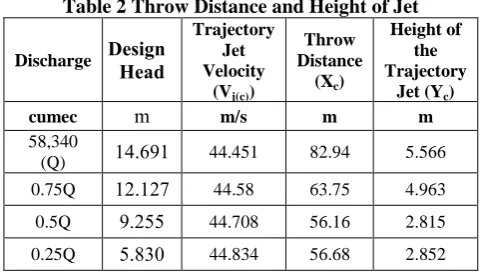
[image:2.595.92.246.98.231.2] [image:2.595.306.547.475.611.2]The study aims to estimate the impact point of the trajectory jet ejecting at the lip level of the flip bucket with the proposed eq. (5) and eq. (7) as detailed in Table 2 below.
Table 2 Throw Distance and Height of Jet Discharge ngiseD
dneH
Trajectory Jet Velocity
(Vj(c))
Throw Distance
(Xc)
Height of the Trajectory
Jet (Yc)
cumec m m/s m m
58,340
(Q) 196.41 44.451 82.94 5.566
0.75Q 126121 44.58 63.75 4.963
0.5Q 46299 44.708 56.16 2.815
0.25Q 968.5 44.834 56.68 2.852
B.
Simulation Analysis:International Journal of Innovative Technology and Exploring Engineering (IJITEE) ISSN: 2278-3075,Volume-8 Issue-12, October 2019
For the simulation of spillway, the geometry was created in a two dimensional plane with Cartesian coordinate system. The simulations were performed on the 1:100 scale model of the spillway section of Nagarjuna Sagar Dam by considering Froude’s model law. Fine mesh was adopted for better accuracy of the results. The mesh was made of 0.01 cell size and 95,000 number of nodes of paved sections, made up of Quadra-triangular cells. The Fluent solver was adopted to determine the spillway parameters for four different discharges viz., maximum discharge of Q = 58340 cumec, 0.75Q, 0.5Q and 0.25Q.
For the two dimensional steady state incompressible flow, the Reynolds-Averaged Navier-Stokes equations are given below [4]. 0 y v x u
(8)
' v ' ρu y u μ y ' u ' ρu x u μ x x p y u v x u u
ρ (9)
' ' ρv'v'
y v μ y v ρu x v μ x y p y v v x v u
ρ (10)
In the eq. (9) & (10), the terms -u’u’, -v’v’ and -u’v’ behave like stress terms, the first two terms are normal stresses and the last term is a shear stress.
j k T j j i ij j j x k σ v v x ε x U τ x k U tk (11)
The first term on the LHS of eqn. (11) represents the rate of change of ‘k’ and the second term explains the transport the ‘k’ b convection. While the first term on the RHS s mbolizes the transport of ‘k’ b diffusion, the second term demonstrates the rate of destruction of ‘k’ and the third term illustrates the rate of production of ‘k’.
Dissipation Rate:
j T j e j i il e j j x k v v x k C x U k C x Ut
2 2 1 (12)
The production and the dissipation terms of eq. (12) are formed from eq. (10) scaled by /k and multiplied by empirical constants and wall damping functions (Ce1 and
Ce2). An additional damping function must be included for
the eddy viscosity in the k- equation by near walls so that k and will have the proper behavior in the near region. The Closure coefficients and auxiliary relations are given below [5]:
Ce1 = 1.44, Ce2 = 1.92, σk = 1.0, σε = 1.3, ω = ε/(Cµk).
The Semi Implicit Method for Pressure Linked Equations (SIMPLE), was adopted which is designed exclusively for turbulence simulations. Each velocity was assigned for solving various equations such as Continuity, X - Velocity, Y - Velocit , k and ε – equations, leading to convergence. For each time step 20 iterations were taken to attain convergence.
The computational time (flow to fall into the bucket and hit on the downstream side of the spillway) ranged from 4 to 6 hr
[image:3.595.50.290.236.337.2]for attaining the convergence criteria. The simulations were carried out using the scale down velocities over the crest of the spillway as detailed in Table 3 for various discharges. The required solution was observed to converge for 900 time steps and at 6500 iterations.
Table 3 Flow Parameters Description Discharge
(cumec)
Scale down flow velocity
(Vs) (m/s)
Q 58,340 0.8309
0.75Q 43,755 0.7569 0.5Q 29,170 0.6631 0.25Q 14,585 0.5282
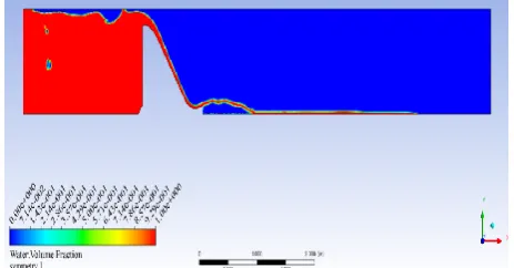
[image:3.595.312.544.365.486.2]In the present analysis, widely adopted and user friendly k-ε turbulence model was used to simulate the flow by Volume of Fluid (VOF) approach. The volume fraction of water was computed for the cells packed between the upstream and downstream of the spillway. In simulation analysis, the profile of the spillway was assigned the properties of smooth metal surface. The manning’s n value for the smooth metal surface (0.012) and smooth concrete (0.011) is approximately the same. Hence, the material properties assigned to the model while performing simulation studies may not contribute significantly to the end result. For the maximum discharge of 58,340 cumec, the contours of volume fraction obtained are shown in Fig. 2. It can be read from Fig. 2 that, red color indicates the path traced by water.
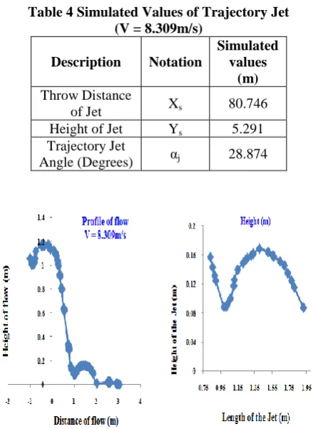
Fig 3 Contours of Trajectory Jet Length and Height The simulated values of depth of flow in the bucket along with the throw distance, height and angle of the trajectory jet are shown in Table 4.
Table 4 Simulated Values of Trajectory Jet (V = 8.309m/s)
Description Notation
Simulated values
(m) Throw Distance
of Jet Xs 80.746
Height of Jet Ys 5.291
Trajectory Jet
Angle (Degrees) αj 28.874
Fig. 4 (a) UDF Flow Profile over Spillway (b) UDF Trajectory Length and Height, V = 8.309 m/s The contours of velocity magnitude are highlighted in Fig. 5. It is evident from the Fig. 5 that, the flow velocity gradually increases towards the invert level of the bucket. This is due to the fact that, the potential energy of flowing water is getting converted to kinetic energy. The blue colour in Fig. 5 indicates that, the water in the reservoir on the upstream side is stagnant. Hence, its velocity is indicated as zero. From Fig. 5 it is seen that, the flow velocity on the downstream side of the spillway profile is having a value of 25.0 m/s at the inflection point. This value is in agreement with the theoretically computed flow velocity of 25.1 m/s at the same point. Moreover, negative pressures are generally likely to occur over the crest of the spillway because of unevenness caused by abrupt offsets, and/or depressions/projections. However, the negative pressures caused by them are very small, and will not approach absolute pressures that can provoke cavitation. From Fig. 5 it is also evident that, the flow velocities over the spillway crest are positive. Hence, the d namic pressure over the crest can’t be negative. As a consequence of this, the chances of inducing cavitation do not arise.
Fig. 5 Contours of Velocity Magnitude IV. RESULTSANDDISCUSSIONS
Based on the proposed analytical computations and simulation results over the spillway, the following results were deduced.
[image:4.595.57.277.199.500.2]1) The analytical values of velocity at the exit level of the bucket are in good consonance with the simulated values for various discharges as depicted in the Fig. 6.
Fig. 6 Comparative Results of Velocity
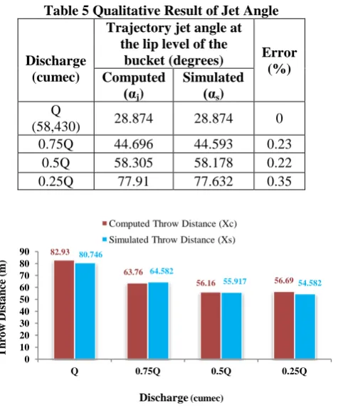
2) The percentage error between the proposed analytical estimates and simulated values for trajectory jet angle is quite small. Therefore, the simulated results of trajectory jet angle were found to be in acceptable harmony with the analytical values as highlighted in the Table 5. According to Cuneyt Yavuz et al [6], the trajectory angle at the impingement area increased for decreasing discharges thereby increasing the jet impact along with the dynamic pressures. The present investigation also supports the above statement.
3) The UDF evaluated simulated results were compared with the proposed analytical values. The trajectory length of the jet ejecting out at the lip level of the bucket were analyzed for four selected discharges. They are observed to have the same agreement as stated in Fig. 7.
44.451
44.580
44.708
44.834
44.700 44.670
45.100
44.500
44.000 44.200 44.400 44.600 44.800 45.000 45.200
Q 0.75Q 0.5Q 0.25Q
Computed Velocity at the lip level of the bucket Simulated Velocity at the lip level of the bucket
V
el
o
ci
ty
, m
/s
[image:4.595.307.549.282.452.2]International Journal of Innovative Technology and Exploring Engineering (IJITEE) ISSN: 2278-3075,Volume-8 Issue-12, October 2019
Table 5 Qualitative Result of Jet Angle
Discharge (cumec)
Trajectory jet angle at the lip level of the
bucket (degrees) Error (%) Computed
(αj)
Simulated (αs) Q
(58,430) 28.874 28.874 0 0.75Q 44.696 44.593 0.23
0.5Q 58.305 58.178 0.22 0.25Q 77.91 77.632 0.35
[image:5.595.50.293.376.556.2]Fig. 7 Comparative Results of Trajectory Throw Distance 4) The macro generated UDF simulated results were compared with the computed values of trajectory jet height for four different discharges. They are observed to have the same synchronization as stated in Fig. 8.
Fig. 8 Comparative Results of Height Distance
V. CONCLUSION
From the literature it is observed that, limited studies were carried out towards estimation of spillway flip bucket parameters. The proposed equations for the trajectory length (X) and height (Y) of the jet above the lip level of the bucket were developed based on the results interpreted from user-defined function. A macro was generated for VOF - multiphase analysis in this regard.
The percentage of error between simulated and analytical results for trajectory jet angle was less than 0.5%. Based on the strong agreement of simulation results with analytical approach, the equations for height and length of the jet trajectory are proposed. From the analysis, the comparative results for length and height of the trajectory jet were observed to have an error less than 5%. Therefore, it is suggested to adopt the proposed equations for analytical estimation of spillway flip bucket parameters
REFERENCES
1. Simpiger B. M, Bhalerao A. R, Estimation of Throw Distance in the
Design of Ski-Jump Bucket, International Journal of Scientific & Engineering Research, 7(3), 2016, 1241 – 1221.
2. Gopal Rao M, Nagarjunasagar – The Epic of A Great Temple of
Humanity, Bharatiya Vidya Bahvan, Bombay, Chapter-7, Design and Instrumentation, 1979, 137 – 140.
3. Stephen T. Maynord, General Spillway Investigation (Hydraulic
Model Investigation), Technical Report, HL-85-1, Department of Navy, Waterways Experiment Station, U.S. Army Corps of Engineers, Mississippi, 4 - 10.
4. Abdulnaser Sayma. Computational Fluid Dynamics: Venus
Publishing, ApS (www.bookboon.com), 2009.
5. Wilcox, David C. Turbulence Modeling for CFD, DCW Industries,
Inc. California, 2006.
6. Cuneyt Yavuz, Ali E. Dincer, Ismail Aydin, Head Loss Estimation for
Water Jets from Flip Buckets, The International Journal Of Engineering And Science, 5(11), 2016, 48 – 57.
AUTHORSPROFILE
DR. (Ms.) SVSNDL PRASANNA, has obtained her Ph.D. degree from Osmania University, Hyderabad. She received her degree in the year 2019 for her work entitled
‘Turbulence Modeling for Selective H draulic
Engineering Applications’. She has 12 ears of teaching and research experience. She has published about 8 National / International Journals and more than 5 in International and National Conferences. She has delivered 5 guest lectures in reputed Government and Private Institutions.
Prof. N. Suresh Kumar, has obtained his Ph.D. degree from IIT., BOMBAY. He received his degree in the year 1998 for his work entitled ‘Jet Mixing in Flocculators’
under the guidance of Prof. B. S. Pani and Prof. S. G.
Joshi. He has more than 30 years of teaching and research experience. He transferred the technology developed as a part of his Ph.D. program from lab to land. Provided the process design and
drawing for a Jet Flocculator - a component in primary treatment unit of
Kitchen effluent treatment plant for ANNAMRITA- ISKCON FOOD RELIEF FOUNDATION, Mumbai. The project site is located at Kanchad
village near Wada, Maharashtra. (Completed). He has published 10
National / International Journals and more than 20 in International and National Conferences. He has delivered more than 30 guest lectures in reputed Government and Private Institutions
82.93
63.76
56.16 56.69
80.746
64.582
55.917 54.582
0 10 20 30 40 50 60 70 80 90
Q 0.75Q 0.5Q 0.25Q
Computed Throw Distance (Xc)
Simulated Throw Distance (Xs)
Discharge (cumec)
T
h
ro
w
D
ist
a
n
ce
(
m
)
5.566
4.963
2.815 2.852
5.291
4.744
2.992 2.973
0 1 2 3 4 5 6
Q 0.75Q 0.5Q 0.25Q
Computed Height of the Jet (Yc) Simulated Height of the Jet (Ys)
Discharge (cumc)
T
h
ro
w
Hei
g
h
t
(m