original

Matchmaking Scientific Workflows in Grid Environments

1

Community Grids Lab

2

Department of Computer Science

3

School of Informatics Indiana University

Bloomington, IN 47404

[email protected], [email protected], and [email protected]

Abstract In this paper we analyze the scientific workflow matchmaking problem in Grid environments and combine workflow mapping and scheduling. Based on the characteristics of Grids, a new resource model is proposed. Motivated by the observations that not all jobs can run on all resources and that resource-critical jobs should be considered with their

ancestor and descendant jobs when mapping, a novel resource-critical algorithm is designed based on a new Grid resource model. By means of experiments, it is shown to have good performance.

Keywords: Grid Computing, Workflow, Resource Model, Matchmaking algorithm

1.

Introduction

Grids are attracting more and more scientific applications, such as those in earthquake science [1], computational chemical informatics [2], physics, astronomy, etc. These applications often include parallel computing and the processing of large scale data in steps. Because of the various requirements of jobs, the large number of jobs and the heterogeneity of

resources, mapping large-scale collaborative workflows onto the heterogeneous resources in Grids is a non-trivial problem. In the QuakeSim project [1], we are working on mapping scientific workflows onto TeraGrid resources for execution.

There are some jobs which cannot run on all resources. For example, a the case of a program named GeoFEST [3], which can only run on IA-32 architecture and requires Pyramid library; only 3 out of 15 TeraGrid resources can satisfy its requirements. There are already some works in the workflow scheduling field but this kind of problem is not directly addressed.

In this paper, according to our target earthquake workflows and execution environment, TeraGrid [4], we make a few distinct assumptions. First, many works [5, 6] assume that a machine can only execute one job at the same time, i.e. it is

exclusive. This holds true on a single processor but not for batch queuing systems in a cluster. Once two jobs have no data or logic dependency, they can probably run simultaneously on a computing resource (if not exceeding any limit). Based on this observation, we propose a new resource model. Second, previous works only assume that jobs can run on every resource and

that the heterogeneity of resources only makes jobs’ running time different. While in realistic Grids, due to access control policies, different software installation or version incompatibility, and particular hardware required (e.g. special visualization

cards), etc, it’s commonly seen that some jobs can never run on certain machines. This phenomenon makes the workflow scheduling in Grids quite unique and challenging. This is also why we call our workflow mapping “matchmaking”, since it is not only scheduling the jobs onto resources, but also prior to that it matches the jobs with the resources which satisfy their

requirements. The term “matchmaking” is borrowed from Condor [7], but in Condor matchmaking is only finding resources for single jobs, while our matchmaking system is aimed at for finding resources for workflows. Under this assumption, the

jobs which can run on every resource are more flexible than the resource-critical jobs which can only run on just a few resources. For a resource-critical job, considering the more resource-flexible jobs before and after it as a group for mapping should be better than mapping them individually. This is the key idea for our resource-critical workflow matchmaking

Our main contributions are as follows. First, we propose a new resource model for cluster node in Grids; second, we propose a resource-critical algorithm for workflow matchmaking, which is proven to have good performance by experiments.

The remainder of the paper is organized as follows. Section 2 describes related work. Section 3 shows the system

architecture of the workflow matchmaking system in Grids. The workflow matchmaking problem in Grids is formulized, a resource model is set up and a resource-critical algorithm is proposed in Section 4. In Section 5, the algorithm is evaluated under varying experimental settings. Finally, Section 6 concludes the paper.

2.

Related Work

There is a large amount of work concerning DAG workflow scheduling [8]. In recent years, much work focuses on

scientific workflow scheduling and heterogeneous environments, especially Grids [9, 10, 11, 12, 13, 14, 15 and 16]. Most of them only assume that jobs can run on every resource and that the heterogeneity of resources mainly makes jobs’ running time different. While in realistic Grids, due to access control policies, different software installation or version incompatibility,

storage limitation, etc, it is commonly seen that some jobs can never run on certain machines. Some of them, such as HEFT in [17] and the hybrid heuristic in [6], are based on the assumption that no two jobs can be executed at the same time on a

resource. But in Grid environments, the common resources are clusters, in which multiple jobs can run concurrently. In [18], the authors do take the storage constraint on resources into consideration. This can be easily incorporated into our model by stipulating that if a resource cannot accommodate the data files needed for a job, the job cannot run on the resource.

3.

System Architecture

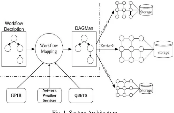
Fig. 1. System Architecture.

This work is intended to map scientific workflows onto resources in Grids. Fig. 1 shows our implementation of a

workflow matchmaking system, which reuses services from several existing projects. Since the target execution environment is TeraGrid, which use the Globus Toolkit [19] to provide remote job submission and management, we select Condor

DAGMan [20] to describe and submit workflow jobs with its support by Condor-G [21]. That is, we use Condor-G as a client to Globus services.

Two services are used to get resource information required by workflow matchmaking. Static information, e.g. CPU

number, OS, etc, is retrieved through GPIRQuery, the web service provided by GPIR [22]. Dynamic information, such as network bandwidth, host load, etc, is acquired by NWS [23]. QBETS [24] can predict the execution time of jobs on resources.

All these services are installed and running on TeraGrid to serve queries.

The input of the workflow mapping system is a description of the workflow. It follows the grammar of DAGMan and Condor-G on submitting, except that it does not need to specify the actual location information about which resources the

4.

A Resource-Critical Algorithm for Workflow Matchmaking

4.1 Problem Statement

The core of a workflow matchmaking system is an algorithm for workflow matchmaking. This sub-section gives the

formal description of the optimization problem.

Given a DAG (Directed Acyclic Graph) of the workflow representation of the application, G = (V, E), V = {v1, …, vN} is the set of jobs in the workflow and N is the total job number. volij denotes the volume of data generated by i and is required by j, i, j V and ij E.

Let the set of Grid resources be R = {r1, …, rm} and M is the number of resources (machines) in the Grid. cij is the computation cost of job i on resource j. Let C(G, R) ={cij|i V, j R}. If job i cannot run on resource j, cij is infinity.

In batch systems, after they are submitted, jobs typically have to wait some time before actually running; wij is the waiting time for job i on resource j. Let W(G, R) ={wij|i V, j R}. Using QBETS [24] we can get predicted waiting times for jobs on TeraGrid resources.

trij is the transfer rate from resource i to j, i, j R. is the communication cost between i and j, when i is executed

on k and j on l, and is derived by dividing , i, j V, k, j R. When i and j are executed on the same resource, the

communication cost is zero. Let T(G, R) = { |i, j V, k, l R}.

Let parents(v) be the parent(s) of the job v and children(v) be the child(children) of the job v, v∈V. These functions can be inferred from the DAG. Here, we assume that the DAG has a single entry node v0 which has no parent, i.e. parents(v0) = and a single exit node vN-1 which has no child, i.e. children(vN-1) = ; any of the other nodes has at least one parent and one child.

Assume the function map(v): V→R is the mapping from the jobs to the resources.

Let EST(v, r) and EFT(v, r) be the earliest start time and earliest finish time of job v on resource r respectively. For the entry node, EST(v0, r) = 0, r R. For the other jobs, EST(v, r) means the earliest time at which all of v’s parent jobs have finished, the data it requires have been transferred to resource r and it is ready to run. Here, we assume that the data transferring and the job waiting can be concurrent. Thus it can be derived that

. Here u is a parent of v, is the

earliest finish time of node u and is the bigger of the transmission time from u to v and the waiting

time of v on resource r. EFT(v, r) = EST(v, r) + cv, r. The makespan, i.e. the overall execution time of the workflow, is the earliest finish time of the exit job, vN-1, i.e. EFT(vN-1).

The workflow matchmaking problem is summarized as follows:

Given {G, R, C(G, R), W(G, R), T(G, R)}. Select the mapping map(v) to minimize the makespan of the workflow, EFT(vN-1).

4.2 Resource Model

In early work, resource in a heterogeneous computing environment is modeled as a single processor on which no two jobs can run concurrently. While in Grids, the computing resources are mainly clusters, many but not an infinite number of

jobs can run at one time. We propose a new resource model to describe resources in workflow matchmaking in Grids.

Each node in a Grid has a capability number, such as the CPU number of the cluster, and each job has a required capability number, such as the number of CPUs it needs. At any time, the sum of the required capability numbers of the jobs

4.3 Mechanism and Algorithm

Since it has been proven that the workflow matchmaking problem is NP-complete, we try to find a good heuristic to solve it.

The key idea of the algorithm is to exploit the fact that some jobs can only run on certain resources, which is quite different from the assumption in previous work. For example, in the workflows of QuakeSim project there is a program named GeoFEST [3], which can only run on IA-32 architecture and requires Pyramid library; while only 3 out of 15 TeraGrid

resources can satisfy its requirements. When scheduling a job, existing algorithms only consider the schedule time of this job and previous jobs. If the later jobs can only run a few resources and are not taken into consideration at the scheduling of jobs

before it, the result might be less optimal.

The proposed algorithm is given in Fig. 2. The input of the algorithm is a DAG G and two matrices: W gives the execution cost of each node on each machine and C gives the communication cost between two nodes/jobs connected by an edge on all combinations of different resources where two nodes can run (the description of the resource and the requirement of the job match); the cost is zero if the two jobs are executed by the same machine.

Since a job may not run on all resources, we define MR(v) as the match ratio of the number of resources on which the job v can run and the number of all resources, . By checking the computation cost array, it is easy to get MR(v) by calculating the number of cvr which is not equal to infinity, .

The algorithm consists of three phases: ranking, group creation, scheduling a group.

Fig. 2. The resource-critical workflow matchmaking algorithm.

In the first step, a weight is assigned to each node and edge of the DAG, which is the mean value of all possible values.

The weight of a node is the mean of its computation cost on all matched resources. As stated in the previous section, in most Grids, such as Condor-G and Globus Toolkit based Grids, the data transferring and the job waiting can be concurrent, thus the weight of an edge should be the mean of the maximum of the communication cost and the waiting time of all possible

combinations of resources (a pair of resources is a possible combination for an edge only if both of the nodes associated with the edge can run on the corresponding resource).

Using this weight, upward ranking is computed and a rank value is given to each node. The rank value, ranki, of a node i is recursively defined as follows:

,

Where nwi is the weight of node i, children(i) is the set of children of node i and ewij is the weight of the edge connecting node i and j.

In the second step, nodes are sorted in non-ascending order of their rank values. Tie-breaking is done randomly. Based on this order, nodes are divided into groups. The first node (i.e. the node with the highest rank value) is added to a group

numbered 0. Check all its children if all ancestors of the child are grouped, i.e. which have been assigned resources when this

group is being mapped, and the match ratio of the child is below a certain valve . If so, add the child node into the group, 1. Set the computation costs of jobs and communication costs of edges with mean values.

2. Compute the rank for all jobs by traversing DAG upward, starting from the exit node. 3. Sort the jobs in a non-ascending order of the rank values.

4. Group nodes. 5. G0 = { }; i = 0.

6. Scan nodes in the order of their rank values.

7. If current node v has not been grouped 8. then

9. Add v to Gi.

10. For all v’s descendants, u

11. If all ancestors of u have been grouped and all nodes on the path from v to u is in Gi and u’s match ratio MR(u) <

12. add u to Gi.

13. Endfor 14. i++; Gi = { }. 15. Endif

16. Keep scanning until there are no more nodes. 17. For all groups, Gi, in ascending order of i.

18. Schedule the jobs in Gi.

mark it as grouped and check its children further on. If no additional such node is found, make the next ungrouped node as a new group, and so on. The outcome of this process is a set of ordered group, each of which consists of a node and its

descendants on the path to which the match ratios of the nodes are all lower than the valve .

In the third step, a group of nodes are mapped, where any algorithm for scheduling a DAG could be used. Since when scheduling a group, the mapping is probably incomplete, the makespan of the whole workflow is not a proper metric to value different assignments. Given a mapping, an end node is defined as a node which either has no children or whose children

have not all yet been mapped. Comparing the two mappings, the one with the smaller largest EFT of all end nodes is preferred; if they have the same largest EFT, the one with the second smaller EFT is better; and so on. If all EFTs of the end

nodes are the same, choose either of them randomly. So far, we adopt an enumerative algorithm to try all combinations of resources for a group and choose the one with the best EFTs of all end nodes.

On one side, with the valve properly set, the size of a group is not large; on the other side, since the match ratios of nodes in a group, except the ancestor, are lower than a constant , the number of combinations of resource assigning is not high. The pruning technology in branch and bound algorithms can also be used to reduce time. In practice, the running time is

insignificant, since there are only low-cost operations involved in the algorithm.

4.5 Comparative Algorithm

Since we adopt a different resource model and different assumptions, most of the existing workflow scheduling

approaches are not applicable. The minimum EFT algorithm is simple and easy to be extended to our resource model as well as satisfy our assumptions. Maybe some other algorithms can also be adapted to our resource model and assumptions, but

revision of their core algorithms is needed. Much effort and time will need to be expended on this revision and we plan to undertake this in future.

In the minimum EFT algorithm, nodes are sorted in non-ascending order of their rank values in the same way as the first

two steps of the resource-critical algorithm, shown in section 4.2. Then nodes are scanned in the order of their rank values. For the each current node, the resource which makes it finish earliest is always chosen.

5.

Experimental Evaluation

This section evaluates our resource-critical workflow matchmaking algorithm against the minimum EFT algorithm. First, the settings of the experiments are described. Then we define the metrics for evaluation. Finally the simulation results are

shown and discussed. This section describes results from modeling that we have used to validate our algorithm for typical usage scenarios in the QuakeSim and CICC project, which involve parameter sweeps (detailed finite element models of

earthquake faults in the Western United States, small molecule structure calculations and docking onto proteins). The individual nodes in the sweep involve parallelized codes and are computationally intensive.

5.1 Settings

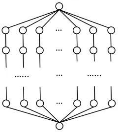
Fig. 3. The structure of a parameter sweep DAG.

Many factors influence the performance of a workflow matchmaking system in Grids.

…

…

…... 

…

…... 

z DAG Generator

We generate parameter sweep DAGs, whose structure is shown in Fig. 3. Every DAG has one start node and one end node. Jobs on the same level in different branches have same resource requirements, i.e. they can run on the same set of

resources, and similar execution time. We vary the branch number and the depth respectively from 4 to 12 and from 8 to 24, and correspondingly the number of node are from 34 to 290.

z Heterogeneity Model

The heterogeneity model we adopt is based on the loosely consistent heterogeneity model, also called the proportional computation cost model in [5], and incorporates the practical resource information from TeraGrid. In the original loosely

consistent heterogeneity model, a random number between 0.5 and 1 is first generated as a factor indicating the computational power of each machine; then the cost for a given job on a given machine within 5% of the product of this number and a baseline computation cost for each job is selected randomly. In our revised model, there are 15 resources

and instead of being generated randomly, the factors indicating their computational power are the same as they are in TeraGrid.

The base execution time of a job is chosen using a random uniform distribution over the interval [10, 100]. z Match ratio

This is a new factor introduced by considering the fact that some jobs can never run on certain resources. The match

ratio for a job is the ratio of the matched and total resource numbers. The ratios are randomly generated among the values from 0 to 1 while a job at least has one matched resource on which it can run.

z Communication Bandwidth

The communication bandwidth between any two resources is a random number between 5M/s and 300M/s. This is the bandwidth range we measured among resources in TeraGrid.

z Communication-to-Computation-Ratio (CCR)

CCR of a parallel program is defined as its average communication cost divided by its average computation cost on a

given system. If a graph is with a very low CCR, it can be considered as a computation intensive application. z Match Ratio Threshold (MRT)

This value is used by the resource-critical algorithm to decide which nodes should be grouped together for mapping. If

the MRT is so small that no resource’s match ratio below it, every node is a group and the resource-critical algorithm acts the same as the minimum EFT algorithm. If the MRT is too large, the groups will expand, for example, if MRT = 1,

all nodes will form one group; to find the best solution for a big group is time consuming. In the experiments, we set MRT from 0.1 to 0.5.

For a given branch number and a given depth, we generate 200 DAGs with their own job computing times, job-resource

match ratios and resource communication bandwidths. A DAG with its corresponding job computing times, job-resource math ratios and resource communication bandwidths is called a case. With each combination of branch number, depth, CCR

and MRT, these two algorithms will be run on the 200 cases of the corresponding branch number and depth.

5.2 Metrics

Two metrics are used to evaluate the algorithms – difference ratio and average improvement ratio. z Difference Ratio

First, we define a metric named Normalized Schedule Length (NSL) [25], also called Schedule Length Ratio (SLR) [17].

NSL is the ratio of the makespan divided by a fixed cost of the critical path.

∑

=

CP ni

w

n

L

NSL

)

(

no communication cost is considered, such a lower bound is probably not possible to achieve and the calculated schedule length should be larger than this bound.

Our resource-critical algorithm (Section 4) does not always outperform the minimum EFT algorithm. The difference

ratio is the ratio of the difference of NSLs for two algorithms and the bigger NSL of two. If a difference ratio is below zero, the NSL of the resource-critical algorithm is larger than that of the minimum EFT algorithm; if it is above zero, it shows that the resource-critical algorithm has a better mapping result than the EFT algorithm if it is equal to zero, the

two algorithms are deemed to perform the same. z Average Improvement Ratio

As its name shows, the average improvement ratio is the average of difference ratios of all cases in a certain setting.

5.3 Results

In the first set of experiments, the branch numbers and the depth numbers of the DAGs are all set as 4 and 8 respectively,

i.e. the node number is 34. The other settings have similar results.

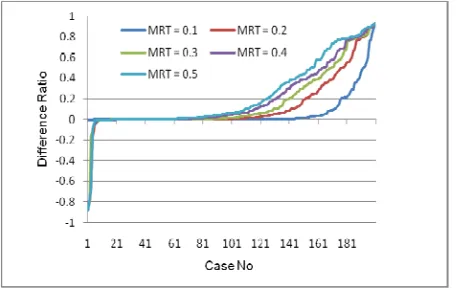
The influence of Match Ratio Threshold (MRT) on difference ratio is shown in Fig. 4. Here CCR

(Communication-to-Computation-Ratio) = 1.0. It can be noticed that in some cases, the resource-critical algorithm performs worse than the minimum EFT algorithm; in some cases, they perform the same; in most cases, it outperforms the minimum EFT algorithm. The reason for these underperforming cases is that when mapping a group, the resource-critical algorithm

only considers information about the nodes in the group and the nodes which have already been mapped. It always minimizes the finish times of current nodes while sometimes compromising the finish times of current nodes can achieve better finish

time of the children nodes in the long run.

In Fig. 5, the average improvement ratios of 200 cases are shown. As the MRT grows, the average improvement ratio of the resource-critical algorithm over the minimum algorithm grows from 6.31% to 23.13%. Combining these two figures

together, it can be concluded that the bigger the MRT is, the better the difference ratios are. MRT is used to control which nodes should be grouped and mapped together: the bigger it is, the more nodes could be grouped together, thus there is a

better chance to find a better mapping.

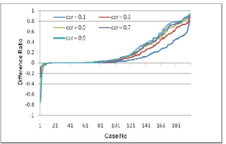
Fig. 6 gives the difference ratios of 200 cases under different CCR values with MRT = 0.5. For all CCRs, in 7.5% - 8.5% cases among all 200 cases the resource-critical algorithm performs worse than the minimum EFT algorithm; in 13% - 19%

cases they perform the same; in 72% - 78% cases, the former outperforms the latter. In Fig. 7, the average improvement ratio increases from 11.65% to 23.69% as the CCR increases. This shows that the resource-critical algorithm works better where

communication cost plays a heavier role. In the extreme circumstance in which there is no communication cost, our algorithm will degrade to the minimum EFT algorithm.

Fig. 4. Difference ratio under various MRTs with CCR=1. Fig. 5. Average improvement ratio under various MRTs

Fig. 6. Difference ratio under various CCRs with MRT=0.5. Fig. 7. Average improvement ratio under various CCRs with

MRT=0.5.

Fig. 8. Average improvement ratio under various branch numbers with CCR=1.0, MRT=0.5, depth=24.

Fig. 9. Average improvement ratio under various depths with CCR=1.0, MRT=0.5, branch number=4.

In the second set of experiments, we discuss the influence of the branch number, the depth and the node number on the performance of these algorithms. Here CCR (Communication-to-Computation-Ratio) = 1.0 and Match Ratio Threshold (MRT) = 0.5.

First, the depth of the workflows is set as 24 and the branch number varies from 4 to 12. As Fig. 8 shows, the average improvement ratio does not deviate much from 45%. This is decided by the characteristic of the parameter sweep applications:

the branches are independent from each other except that they share the same start and end nodes; thus the branch number does not much influence grouping and correspondingly does not much influence mapping.

Second, we set the branch number of the workflows as 4 and vary the depth from 8 to 24. As seen from Fig. 9, the

average improvement ratio of the resource-critical algorithm over the minimum EFT algorithm increases from 23.13% to 43.45% as the depth increases. This is because the greater the depth, the more chances there are that more nodes can be

grouped together to find the best mapping by trying all possible combinations.

6.

Conclusion and Future Work

In this paper, we investigate the problem of matchmaking scientific workflow onto resources in Grid environments. We

combine the workflow mapping and scheduling together and present a new resource model to formalize the problem. By exploiting the fact that some jobs can only run on some resources, we propose a novel algorithm of resource-critical

workflow mapping, which take advantage of the fact that some jobs can only run on a small number of resources and that mapping them together with their ancestor jobs can achieve better mapping results. By means of modeling experiments, we discuss the factors affecting the performance of the algorithm. And it has been demonstrated that the resource-critical

algorithm outperform the minimum EFT algorithm in various conditions.

algorithm (Section 4.3) for realistic scenarios. We are currently working to complete the deployment of the system for specific high performance parameter sweep problems from the QuakeSim and CICC projects.

This work is funded by the National Aeronautics and Space Administration’s Advanced Information Systems Technology

program.

References

[1] The QuakeSim project. http://quakesim.jpl.nasa.gov/.

[2] X. Dong, K. Gilbert, R. Guha, J. Kim, M. E. Pierce, G. C. Fox and D. J. Wild, Smart mining of drug discovery

information: A web service and workflow infrastructure, Submitted to Journal of Chemical Information and Modeling October 2006.

[3] Geophysical finite element simulation tool. Http://www.openchannelfoundation.org/projects/GeoFEST/.

[4] C. E. Catlett, TeraGrid: A foundation for US cyberinfrastructure, Proceedings of NPC 2005. http://www.teragrid.org. [5] H. Zhao and R. Sakellariou, An experimental investigation into the rank function of the heterogeneous earliest finish

time scheduling algorithm, Proceedings of Euro-Par’03, LNCS 2790, Springer, 2003.

[6] R. Sakellariou and H. Zhao, A hybrid heuristic for DAG scheduling on heterogeneous systems. Proceedings of IPDPS’04.

[7] D. Thain, T. Tannenbaum, and M. Livny, Distributed computing in practice: The Condor experience, Concurrency and Computation: Practice and Experience, Vol. 17, No. 2-4, pages 323-356, February-April, 2005. http://www.cs.wisc.edu/condor/.

[8] Y. Kwok and I. Ahmad, Static scheduling algorithms for allocating directed task graphs to multiprocessors, ACM Computing Surveys, 31(4): 406-471, 1999.

[9] R. Sakellariou and H. Zhao. A low-cost rescheduling policy for efficient mapping of workflows on Grid systems, Scientific Programming, vol. 12, no. 4, pp. 253-262, December, 2004.

[10]J. Blythe, S. Jain, E. Deelman, Y. Gil, K. Vahi, A. Mandal and K. Kennedy, Task scheduling strategies for workflow-based applications in Grids, Proceedings of IEEE International Symposium on Cluster Computing and Grid (CCGrid), 2005.

[11]H. Zhao, R. Sakellariou, Advance reservation policies for workflows. Proceedings of JSSPP 2006: 47-67.

[12]A. Mandal, K. Kennedy, C. Koelbel, G. Marin, J. Mellor-Crummey, B. Liu and L. Johnsson, Scheduling strategies for

mapping application workflows onto the Grid, Proceedings of IEEE International Symposium on High Performance Distributed Computing (HPDC 2005).

[13]M. Wieczorek, R. Prodan and T. Fahringer, Scheduling of scientific workflows in the ASKALON Grid environment,

SIGMOD Record, volume 34(3), September 2005.

[14]T. Ma and R. Buyya. Critical-path and priority based algorithms for scheduling workflows with parameter sweep tasks

on global Grids. Proceedings of the 17th International Symposium on Computer Architecture and High Performance Computing (SBAC-PAD 2005), Oct. 24-27, 2005, Rio de Janeiro, Brazil.

[15]J. Yu and R. Buyya, A budget constraint scheduling of workflow applications on utility Grids using genetic algorithms.

Proceedings of the Workshop on Workflows in Support of Large-Scale Science (WORKS06), Paris, France, 2006. [16]E. Ilavarasan and P. Thambidurai. Low complexity performance effective task scheduling algorithm for heterogeneous

computing environments. Journal of Computer Sciences 3 (2): 94-103, 2007.

[17]H. Topcuoglu, S. Hariri and M. Wu. Performance-effective and low-complexity task scheduling for heterogeneous computing. IEEE Transactions on Parallel and Distributed Systems, vol. 13, No. 3, pp. 260-274, March 2002.

International Symposium on Cluster Computing and the Grid - CCGrid 2007.

[19]I. Foster, Globus toolkit version 4: Software for service-oriented systems. Proceedings of IFIP International Conference on Network and Parallel Computing, Springer-Verlag LNCS 3779, pp 2-13, 2005. http://www.globus.org/.

[20]Condor DAGMan. http://www.cs.wisc.edu/condor/dagman/.

[21]J. Frey, T. Tannenbaum, I. Foster, M. Livny, and S. Tuecke, Condor-G: A computation management agent for multi-Institutional Grids", Journal of Cluster Computing volume 5, pages 237-246, 2002.

http://www.cs.wisc.edu/condor/condorg/.

[22]J. Alameda, M. Christie, G. C. Fox, J. Futrelle, D. Gannon, M. Hategan, G. von Laszewski, M. A. Nacar, M. E. Pierce, E.

Roberts, C. Severance, and M. Thomas, The open Grid computing environments collaboration: Portlets and services for science Gateways, Concurrency and Computation: Practice and Experience Special Issue for Science Gateways, March 2006. http://gridport.net/services/gpir/.

[23]R. Wolski, N. Spring, and J. Hayes, The network weather service: A distributed resource performance forecasting service for metacomputing, Journal of Future Generation Computing Systems}, Volume 15, Numbers 5-6, pp. 757-768, October, 1999. http://nws.cs.ucsb.edu/ewiki.

[24]D. Nurmi, J. Brevik, and R. Wolski. QBETS: Queue bounds estimation from time series, Proceedings of 3th Workshop on Job Scheduling Strategies for Parallel Processing, June, 2007.