https://doi.org/10.5194/bg-16-347-2019
© Author(s) 2019. This work is distributed under the Creative Commons Attribution 4.0 License.
Modeling oceanic nitrate and nitrite concentrations and isotopes
using a 3-D inverse N cycle model
Taylor S. Martin1, François Primeau2, and Karen L. Casciotti1
1Department of Earth System Science, Stanford University, Stanford, CA, USA
2Department of Earth System Science, University of California, Irvine, Irvine, CA, USA
Correspondence:Karen L. Casciotti ([email protected]) Received: 5 September 2018 – Discussion started: 17 September 2018
Revised: 21 December 2018 – Accepted: 21 December 2018 – Published: 24 January 2019
Abstract.Nitrite (NO−2) is a key intermediate in the marine nitrogen (N) cycle and a substrate in nitrification, which pro-duces nitrate (NO−3), as well as water column N loss pro-cesses denitrification and anammox. In models of the ma-rine N cycle, NO−2 is often not considered as a separate state variable, since NO−3 occurs in much higher concentrations in the ocean. In oxygen deficient zones (ODZs), however, NO−2 represents a substantial fraction of the bioavailable N, and modeling its production and consumption is important to understand the N cycle processes occurring there, especially those where bioavailable N is lost from or retained within the water column. Improving N cycle models by including NO−2 is important in order to better quantify N cycling rates in ODZs, particularly N loss rates. Here we present the ex-pansion of a global 3-D inverse N cycle model to include NO−2 as a reactive intermediate as well as the processes that produce and consume NO−2 in marine ODZs. NO−2 accumu-lation in ODZs is accurately represented by the model in-volving NO−3 reduction, NO−2 reduction, NO−2 oxidation, and anammox. We model both14N and15N and use a compila-tion of oceanographic measurements of NO−3 and NO−2 con-centrations and isotopes to place a better constraint on the N cycle processes occurring. The model is optimized using a range of isotope effects for denitrification and NO−2 oxi-dation, and we find that the larger (more negative) inverse isotope effects for NO−2 oxidation, along with relatively high rates of NO−2, oxidation give a better simulation of NO−3 and NO−2 concentrations and isotopes in marine ODZs.
1 Introduction
Nitrogen (N) is an important nutrient to consider when as-sessing biogeochemical cycling in the ocean. The N cycle is intrinsically tied to the carbon (C) cycle, whereby N can be the limiting nutrient for primary production and carbon dioxide uptake (Moore et al., 2004; Codispoti, 1989). Under-standing the distribution and speciation of bioavailable N in the ocean allows us to make inferences about the effects on other nutrient cycles and potential roles that N may play in a regime of climate change (Gruber, 2008).
There are several chemical species in which N can be found in the ocean. The largest pool of bioavailable N is nitrate (NO−3), a dissolved inorganic species, which can be taken up by microbes for use in assimilatory or dissimila-tory processes. Another dissolved inorganic species, nitrite (NO−2), accumulates in much lower concentrations but is a key intermediate in many N cycling processes. Models of the marine N cycle often include NO−3 and NO−2 together as a single dissolved inorganic N (DIN) pool, or exclude NO−2 entirely (DeVries et al., 2013; Deutsch et al., 2007; Brandes and Devol, 2002). However, NO−2 does accumulate signifi-cantly in oxygen deficient zones (ODZs) in features known as secondary NO−2 maxima, and it is an intermediate or sub-strate in many important N cycle processes occurring there.
ODZs are hotspots for marine N loss (Codispoti et al., 2001; Deutsch et al., 2007), which is driven by processes that result in conversion of bioavailable DIN to dinitrogen gas (N2). The two main water column N loss processes,
den-itrification and anammox, use NO−2 as a substrate. Denitrifi-cation involves the stepwise reduction of NO−3 to NO−2 and then to gaseous nitric oxide (NO), nitrous oxide (N2O), and
ammo-nium (NH+4) to N2using NO−2 as the electron acceptor. NO−2
is also oxidized to NO−3 during anammox, representing an alternative fate for NO−2 in ODZs. Indeed, NO−2 oxidation appears to be prevalent in ODZs, with more NO−2 oxidation occurring than can be explained by anammox alone (Gaye et al., 2013; Peters et al., 2016, 2018b; Babbin et al., 2017; Buchwald et al., 2015; Casciotti et al., 2013; Martin and Cas-ciotti, 2017). NO−2 oxidation results in the regeneration of NO−3 that would otherwise be converted to N2and lost from
the system. The close coupling between NO−3 reduction to NO−2 and NO−2 oxidation back to NO−3, represents a control valve on the marine N budget (Penn et al., 2016; Bristow et al., 2016). Where NO−2 oxidation can outcompete NO−2 re-duction via denitrification and anammox, bioavailable N is retained. Water column N losses may occur primarily where NO−2 oxidation rates are limited by oxygen availability. Thus, understanding the NO−2 dynamics in ODZ waters is critical to assess the N loss occurring there.
The observed NO−3 and NO−2 concentrations alone do not allow us to fully characterize the N cycling processes occurring in a given region. Stable isotope measurements of NO−3 and NO−2 provide additional insight and con-straints on marine N cycle processes. There are two sta-ble isotopes of N: 14N and 15N. The isotopic ratios for a given N species, usually expressed in delta notation as δ15N (‰)=((15N/14N)sample/(15N/14N)standard−1)×1000,
are an integrated measure of the processes that have pro-duced and consumed that N species. Each process imparts a unique isotope effect (ε(‰)=(14k/15k−1)×1000, where
14kand15kare the first-order rate constants for the14N and 15N containing molecules, respectively) that impacts the
iso-topic composition of the substrate and the product (Mariotti et al., 1981). In particular, NO−2 cycling processes have dis-tinct isotope effects, where NO−2 reduction occurs with nor-mal isotopic fractionation (Bryan et al., 1983; Martin and Casciotti, 2016; Brunner et al., 2013) and NO−2 oxidation occurs with an unusual inverse kinetic isotope effect (Cas-ciotti, 2009; Buchwald and Cas(Cas-ciotti, 2010; Brunner et al., 2013). Thus, the isotopes of NO−2 are sensitive to the relative importance of NO−2 oxidation and NO−2 reduction in NO−2 consumption (Casciotti, 2009; Casciotti et al., 2013).
Models of the marine N cycle have employed isotopes and isotope effects in conjunction with N concentrations to eluci-date N cycle processes (Brandes and Devol, 2002; Sigman et al., 2009; Somes et al., 2010; DeVries et al., 2013; Casciotti et al., 2013; Buchwald et al., 2015; Peters et al., 2016). A model can either assume a set of processes and infer the un-derlying isotope effects, or assume isotope effects and infer a set of processes. The latter isotope models are highly depen-dent on the chosen isotope effects used for given processes. Although there are estimates of isotope effects for processes based on both environmental measurements and laboratory studies, there is not always agreement between them. For example, laboratory cultures of NO−2 oxidizers indicate an N isotope effect of 15ε= −10 to −20 ‰ (Casciotti, 2009;
Buchwald and Casciotti, 2010), while measured concentra-tions and isotopes of NO−3 and NO−2 in ODZs indicate that isotope effects closer to−30 ‰ are needed to explain the observations (Buchwald et al., 2015; Casciotti et al., 2013; Peters et al., 2016).
Here we present an expansion of an existing global ocean 3-D inverse isotope-resolving N cycling model (DeVries et al., 2013) to investigate the isotopic constraints on N cycling in ODZs and the impact of these regions on global ocean N isotope patterns. An important step was to include NO−2 and its isotopes as tracers. The addition of NO−2 allows us to in-clude additional internal N cycling processes, as well as a more nuanced and realistic version of the processes occur-ring in ODZs. We used a database of NO−3 and NO−2 obser-vations in order to assess the performance of the model as well as optimize the model N cycle parameters for which we do not have good prior estimates. In the model we employ a variety of isotope effect estimates for three important ODZ processes – NO−3 reduction, NO−2 reduction, and NO−2 oxi-dation – to discern what isotope effects result in the best fit to the observations.
2 Methods
2.1 Inverse N cycle model overview
be-low outlines the dependencies and simplifications employed in this version of the model.
The model’s uncertain biological parameters were deter-mined through an optimization process that minimizes the difference between the modeled and observed NO−3 and NO−2 concentration and isotope data. Computational time limits the number of parameters that we were able to op-timize. We therefore focused our investigation on parame-ters that are poorly constrained by literature values and to which the model solution is most sensitive. In order to deter-mine the parameters for optimization, a sensitivity analysis was performed on each parameter, varying them individu-ally by±10 % and computing the change in the modeled14N and15N. Those parameters that resulted in modeled14N and
15N variability of>5 % were chosen for optimization in the
model. The sensitivity analysis and the optimal values of the parameters contribute to an improved understanding of the cycling of N in the ocean in general and in the ODZs in par-ticular. The optimization process is discussed in further detail in Sect. 2.6.
The sensitivity analysis revealed that the modeled distri-bution of15N was very sensitive to chosen isotope effects, those parameters that control the relative rates of 15N and
14N in chemical and biological processes. There are
litera-ture estimates for each of the isotope effects of interest in this work, although there is often a discrepancy between isotope effects estimated in laboratory studies and those expressed in oceanographic measurements (Kritee et al., 2012; Casciotti et al., 2013; Bourbonnais et al., 2015; Martin and Casciotti, 2017; Fuchsman et al., 2017; Marconi et al., 2017; Peters et al., 2018b). Rather than optimizing the isotope effect values, we have chosen to use multiple cases with different combina-tions of previously estimated isotope effects in order to assess which values best fit the observations.
In addition to the optimized parameters and isotope ef-fects, there were some nonsensitive parameters that were fixed prior to the optimization and whose values were cho-sen using literature estimates (Table 1). Some N cycle pro-cesses are also dependent on prescribed input fields that are not explicitly modeled, such as temperature, phosphate, oxy-gen, and net primary production. These external input fields will be discussed in detail in the relevant sections for each N cycle process.
2.2 Model grid and transport
The model uses a uniform 2◦×2◦ grid with 24 depth
lev-els. The thickness of each model layer increases with depth, from 36 m at the top of the water column to 633 m near the bottom. Bottom topography was determined using 2 min gridded bathymetry (ETOPO2v2) that was then interpolated to the model grid. Our linear N cycle model relies on the transport of dissolved N species (NO−3, NO−2, and DON) in the ocean. For this we use the annual averaged circula-tion as captured by a tracer transport operator that governs
the rate of transport of dissolved species (NO−3, NO−2, and DON) between boxes. The original version of the tracer data-assimilation procedure used to generate the transport opera-tor for dissolved species (Tf) is described by DeVries and
Primeau (2011), and the higher resolution version used here is described by DeVries et al. (2013).
2.3 N cycle
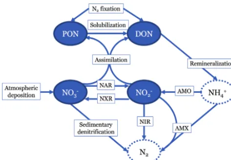
In the N cycling portion of the model, we track four different N species (Fig. 1). There are two organic N (ON) pools: solved (DON) and particulate (PON). There are also two dis-solved inorganic N (DIN) pools: NO−3 and NO−2. We did not explicitly model ammonium (NH+4) because it typically oc-curs in low concentrations throughout the ocean, and scarcity of data (especiallyδ15N data) would make model validation difficult. Although NH+4 has been observed to accumulate to micromolar concentrations in some ODZs (Bristow et al., 2016; Hu et al., 2016), this occurs largely in shallow, coastal shelf regions that are not resolved by the model.
Because we used the concentrations of both14N and15N of each N species to constrain the rate parameters, two sets of governing equations were employed: one that depends on
14N and another that depends on15N. Generally, the rate for 15N processes was dependent on the rate of 14N processes
and an isotopic fractionation factor (α=14k/15k) that is spe-cific to each process and substrate. By solving for steady-state solutions to both14N and15N concentrations, we were able to model global distributions of [NO−3], [NO−2], and their correspondingδ15N values.
2.3.1 N cycle parameterization
We first describe the14N equations and the general format of the N cycle in the model. Each equation is then broken down into its component parts for further explanation of the biolog-ical processes and their parameterization. The15N equations and isotope implementation will be discussed in a later sec-tion.
The governing equations for the 14N-containing DIN (NO−3 and NO−2) and organic N (DON and PON) state vari-ables can be written as follows:
∂
∂t +Tf
h
14NO− 3
i
=J14dep−Jassim,NO3
14 −J
NAR 14
+J14NXR+0.3J14AMX−J14sed, (1)
∂ ∂t +Tf
h
14NO− 2
i
=J14AMO−Jassim,NO2
14 +J
NAR 14
−J14NXR−J14NIR−1.3J14AMX, (2)
∂ ∂t+Tf
h
DO14Ni=σ (J14fix+J14assim,WOA)
Table 1.Non-optimized model parameters.
Parameter Value Reference
b −0.858 Martin et al. (1987)
F0 1.5 mmol N m−3yr−1 DeVries et al. (2013), Capone et al. (2005)
λ 10 mmol N m−3 Holl and Montoya (2005)
T0 20◦C DeVries et al. (2013), Capone et al. (2005) KFe 4.4×10⁻⁵mmol Fe m−3 Follows et al. (2007)
KP 0.005 mmol PO3−4 m−3 Moore and Doney (2007)
rC:N 6.625 Redfield et al. (1963)
KmAMO 3.5 µM O2 Peng et al. (2016)
KmNXR 0.8 µM O2 Bristow et al. (2016)
ONAR2 7 µM O2, 15 µM O2∗ Dalsgaard et al. (2014), Jensen et al. (2008), Kuypers et al. (2005), Kalvelage et al. (2011) ONIR2 5 µM O2, 15 µM O2∗ Bonin et al. (1989), Kalvelage et al. (2011)
OAMX2 10 µM O2, 15 µM O2∗ Dalsgaard et al. (2014), Jensen et al. (2008), Kuypers et al. (2005), Kalvelage et al. (2011)
δ15Ndep −4 ‰ Hastings et al. (2009)
δ15Nfix −1 ‰ Hoering and Ford (1960), Carpenter et al. (1997)
αAMX,NIR 1.016 Brunner et al. (2013)
αAMX,NXR 0.969 Brunner et al. (2013)
αAMX,NH4 1
αAMO 1
αsed 1 Brandes and Devol (1997), Lehmann et al. (2004)
αassim 1.004 Granger et al. (2010)
αremin 1 Casciotti et al. (2008), Möbius (2013)
αsol 1 Knapp et al. (2011)
∗Value used in ETSP O
2sensitivity test (Sect. 4.2).
∂
∂t +Tp
h
PO14Ni=(1−σ )(J14fix+J14assim,WOA)
−J14sol. (4)
The model is designed to represent a steady state, thus the ∂t∂ term is 0. The J terms represent the source and sink processes for each state variable, expressed in units of mmol m−3yr−1and will be described in more detail below. Briefly,J14depis the spatially variable deposition of NO−3 from the atmosphere to the sea surface. In the DIN model equa-tions,Jassim,NO3
14 andJ
assim,NO2
14 represent the assimilation of
NO−3 and NO−2, respectively, by phytoplankton in the upper two box levels. This assimilated NO−3 produces DON and PON, with proportions set by a spatially variable term, σ. Assimilation in the DON and PON equations is represented byJ14assim,WOAand is dependent on 2013 World Ocean Atlas (WOA) [NO−3] interpolated to the model grid. N2 fixation
(J14fix) is split between DON and PON with the sameσ term. NO−3 reduction (J14NAR), NO−2 reduction (J14NIR), NO−2 oxi-dation (J14NXR), and anammox (J14AMX) act on the NO−3 and
NO−2 pools. J14sed represents the removal of NO−3 via ben-thic denitrification.J14sol represents the dissolution of PON into DON.J14reminrepresents the degradation of DON, which feeds into ammonia oxidation (J14AMO) and J14AMX as de-scribed below.
Through the use of theseJterms, the governing equations are all linear with respect to the state variables. However, in order to introduce dependence of rates on the concentra-tions of multiple state variables, for example allowing het-erotrophic NO−3 reduction to be dependent on organic N as well as NO−3, we run the organic N equations and the DIN equations seperately. When [DON] is found in the [DIN] governing equations, that [DON] value has already been de-termined for each grid box from the organic N model. When [NO−3] is found in the DON governing equations, it is drawn from 2013 World Ocean Atlas annual data interpolated to the model grid.
2.3.2 N source processes
Atmospheric deposition and N2 fixation are the two largest
Figure 1.Diagram showing the nitrogen (N) cycle processes rep-resented in the model. Two organic N pools are modeled: partic-ulate organic N (PON) and dissolved organic N (DON). Two in-organic N pools are modeled: nitrate (NO−3) and nitrite (NO−2). N source processes are nitrogen (N2) fixation and atmospheric deposi-tion. N sink processes are sedimentary denitrification, NO−2 reduc-tion (NIR), and anammox (AMX). Internal cycling processes that transform N from one species to another are solubilization, rem-ineralization, assimilation, NO−3 reduction (NAR), ammonia oxida-tion (AMO), and NO−2 oxidation (NXR). Neither ammonia (NH3) nor ammonium (NH+4) are tracked in this model, since they are as-sumed to not accumulate. N2is also not explicitly accounted for in the model.
the only sources of new bioavailable N in the model. We do not consider the third largest source of N, riverine fluxes, in the model due to a lack of coastal resolution and the expec-tation that much of the river-derived N is denitrified in the shelf sediments (Nixon et al., 1996; Seitzinger and Giblin, 1996). Representing these processes may be possible in a future version of the model, but is beyond the scope of the current model, given its coarse resolution near the coasts. Atmospheric deposition
N deposition is assumed to only occur in the top box of the model. We assume that most of the N deposited is as NO−3, and that the other species would be rapidly oxidized to NO−3 in the oxic surface waters.
J14dep=r14depSdep (5)
To calculate J14dep, the atmospheric deposition rate of14N, we use modeled total inorganic N deposition for 1993,Sdep (Galloway et al., 2004; Dentener et al., 2006; data available online at https://daac.ornl.gov/CLIMATE/guides/global_N_ deposition_maps.html, last access: November 2017), which was interpolated to our model grid. This term,Sdep, is then multiplied by a prescribed fractional abundance of 14N in the deposited N (r14dep), which is calculated from the isotopic composition of deposited N (δ15Ndep,−4 ‰; Eq. 6), to yield
the deposition of14N to the sea surface in each box (J14dep). To calculater14depfromδ15Ndep, we first calculater15depusingr15air,
a standard with a value of 0.003676 (Eq. 6; Mariotti, 1983).
r15dep= δ
15N dep
1000 +1
!
×r15air (6)
Then, using the approximation that
15N/14N=15N/(15N+14N), we calculaterdep
14 as (1−r dep 15 ).
The units of Sdep are given in mg N m−2yr−1, which we convert to mmol NO−3 m−3yr−1 by dividing by the depth of the surface box. This source term of N to the model is spatially variable but independent of the modeled N terms. N2fixation
N2 fixation is the other source of new N to the model, and
is assumed to only occur in the top box of the model. It is parameterized similarly to N2fixation in the model of
De-Vries et al. (2013), with partial inhibition by NO−3 (Holl and Montoya, 2005) and dependence on iron (Fe) and phosphate (PO3−4 ) availability (Monteiro et al., 2011).
J14fix=r14fixF0e−NO3,obs/λe Tobs−Tmax
T0 Fe
Fe+KFe
PO4
PO4+KP
(7)
F0is the maximum rate of N2fixation (1.5 mmol m−3yr−1;
Table 1) and is calculated from the estimated areal rate of N2 fixation in the western tropical Atlantic (Capone et al.,
2005) divided by the depth of the top model box. NO3,obsis
the 2013 World Ocean Atlas annually averaged surface NO−3 interpolated to the model grid (Garcia et al., 2013b). The pa-rameterλis an inhibition constant for N2fixation in the
pres-ence of NO−3 (Table 1).
The temperature (T) terms scale the rate of N2 fixation
based on the observed temperature (Tobs), maximum
ob-served sea surface temperature (Tmax), and the minimum
pre-ferred growth temperature forTrichodesmium(T0; Capone et
al., 2005). The temperature data were taken from 2013 World Ocean Atlas annually averaged temperature interpolated to the model grid (Locarnini et al., 2013). We recognize that this will likely provide a conservative estimate of N2
fixa-tion, given the growing recognition of N2fixation outside of
the tropical and subtropical ocean by organisms other than Trichodesmium(Shiozaki et al., 2017; Harding et al., 2018; Landolfi et al., 2018).
Fe is the modeled deposition of soluble Fe interpolated to the model grid (mmol Fe m−2yr−1; Chien et al., 2016) di-vided by the depth of the top model grid box to give units of mmol Fe m−3yr−1. Fe and PO3−4 are assumed to limit N2
fixation at low concentrations via Michaelis–Menten kinet-ics.KFeandKPare their respective half-saturation constants.
δ15Nfix (−1 ‰; Table 1). All of the N2 fixation parameters
are fixed rather than optimized (Table 1). Due to the use of non-optimized parameters and an input NO−3 field rather than modeled NO−3, N2fixation serves as an independent check
that our modeled N cycle produces reasonable N concentra-tions and overall N loss rates. However, N2fixation is not
ex-plicitly modeled here and is instead taken as a fixed, though spatially variable, input field (Fig. S1 in the Supplement). The global rate of N2 fixation produced by this
parameteri-zation is 131 Tg N yr−1, which is in line with several current estimates (Table S1 in the Supplement).
In the model, N2 fixation and NO−3 assimilation
(Sect. 2.3.3) are assumed to be the two processes that cre-ate exportable organic N. A fraction,σ, of this organic N is partitioned into DON rather than PON (Eqs. 3–4). In order to create spatial variability in this constant, we assumed that 1−σ, the fraction of assimilated N partitioned to PON, is equal to the particle export (Pe) ratio. ThisPeratio is the
ra-tio of particle export to primary producra-tion, and is equivalent to the fraction of organic N that is exported from the euphotic zone as particulate matter rather than recycled or solubilized into DON. The Pe ratio is calculated for each model grid
square from the mixed layer temperature (Tml) and net
pri-mary production (NPP) as described by Dunne et al. (2005):
Pe=φTml+0.582 log(NPP)+0.419. (8)
The constant8has a value of−0.0101◦C−1as determined by Dunne et al. (2005). Net primary production estimates (in units of mmol carbon m−2yr−1) were taken from a satellite-derived productivity model (Westberry et al., 2008), annu-ally averaged, and interpolated onto the model grid. Tml is
calculated from the 2013 World Ocean Atlas annual aver-age (Locarnini et al., 2013), which has been interpolated to the model grid. The temperature of the top two model boxes were averaged to giveTml. As temperature increases, thePe
ratio decreases and less PON is exported, resulting in more DON recycling in the surface with several possible explana-tory mechanisms discussed in greater detail by Dunne et al. (2005). As net primary production increases, thePeratio
increases and relatively more PON is exported; net primary production explains 74 % of the observed variance in particle export (Dunne et al., 2005).
2.3.3 Internal N cycling processes Assimilation of nitrate and nitrite
Assimilation accounts for the uptake of DIN and its incor-poration into organic matter in the shallowest two layers of the global model. Since assimilation affects both the organic and inorganic N pools, we must account for it in both sets of model runs. We will first address assimilation in the organic
N model (Eqs. 9 and 10).
J14assim,WOA=14kassim[NO−3]obs (9) 14k
assim=
NPP rC:N[NO−3]obs
(10) Since the organic N model is run first and the assimila-tion rates are dependent on DIN concentraassimila-tions, assump-tions must be made about the DIN field in order to ac-count for assimilation prior to the DIN model runs. Here we used observed [NO−3] from the 2013 World Ocean At-las annual product interpolated to the model grid [NO−3]obs
(Garcia et al., 2013b) to calculate the assimilation rates for DON and PON production (J14assim,WOA). For this assump-tion to be valid, our modeled surface [NO−3] must be close to the observed values, which we will test in Sect. 3.1. The rate constant for assimilation,14kassim, varies spatially
and is determined using observations of surface [NO−3] and satellite-derived net primary production (NPP; Westberry et al., 2008). The rate constant is converted to N units using the ratio of carbon (C) to N in organic matter (rC:N), which we
assume to be 106:16 (Redfield et al., 1963). The value of the rate constant is only nonzero in the top two boxes of the model, where we assume primary production to be occurring. The same rate constant is used in both the organic N and DIN assimilation equations. We also assume from the perspec-tive of organic N that only NO−3 is being assimilated, since NO−2 is present at relatively low concentrations in the surface ocean, and it may be characterized as recycled production. Assimilated N is partitioned between PON and DON using thePe ratio as previously described and shown in Eqs. (3)
and (4).
The setup for assimilation in the DIN model (Eqs. 11 and 12) is similar, but can use modeled [NO−3] and [NO−2] rather than the World Ocean Atlas values. In order to appropriately reflect surface NO−3 and NO−2 concentrations, both NO−3 and NO−2 are assimilated.14kassimis calculated as described
above and is assumed to be the same for both NO−3 and NO−2. We justify using only [NO−3] to parameterize 14kassim
be-cause NO−3 generally makes up the bulk of DIN available for assimilation at the surface, but this assumption will be discussed in more detail below.
Jassim,NO3
14 =
14k
assim[14NO−3] (11)
Jassim,NO2
14 =
14k
assim[14NO−2] (12)
Solubilization
Solubilization is the transformation of PON to DON, and is dependent only on [PON] and a solubilization rate constant (14ksol), which is optimized (Table 2).
J14sol=14ksol[PO14N] (13)
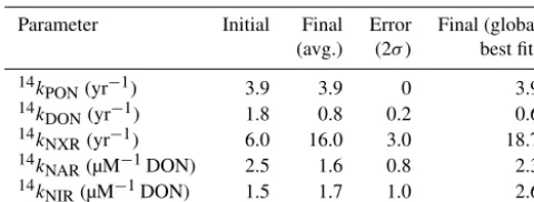
Table 2.Optimized model parameters.
Parameter Initial Final Error Final (global (avg.) (2σ) best fit)
14k
PON(yr−1) 3.9 3.9 0 3.9
14k
DON(yr−1) 1.8 0.8 0.2 0.6
14k
NXR(yr−1) 6.0 16.0 3.0 18.7
14k
NAR(µM−1DON) 2.5 1.6 0.8 2.3
14k
NIR(µM−1DON) 1.5 1.7 1.0 2.6
similar to a Martin curve with exponentb= −0.858 (Table 1; Martin et al., 1987). While in the real world, the length scale for particle flux attenuation is somewhat longer in ODZs compared to oxygenated portions of the water column, and also varies regionally (Berelson, 2002; Buesseler et al., 2008; Buesseler and Boyd, 2009), our model uses a spatially invari-ant14ksol. A spatially variable14ksolthat accounts for lower
apparent values in ODZs is a refinement that could be intro-duced in future model versions.
Remineralization
Remineralization, or ammonification, is the release of DON into the DIN pool. This is parameterized using the concentra-tion of DON and a remineralizaconcentra-tion rate constant (14kremin),
which is optimized (Table 2). J14remin=14kremin
h
DO14Ni (14)
The removal of this remineralized DON, since it does not accumulate as NH+4, is either through ammonia oxidation (AMO) or anammox (AMX), depending on [O2] as
de-scribed below and in Sect. 2.3.4. We use the same reminer-alization rate constant regardless of the utilized electron ac-ceptor (e.g., O2, NO−3). Since particle flux attenuation is
ob-served to be somewhat weaker in ODZs compared with oxy-genated water (Van Mooy et al., 2002), this may slightly overestimate the rates of heterotrophic remineralization oc-curring in ODZs.
Ammonia oxidation (AMO)
AMO uses ammonia (NH3) as a substrate. Since we do not
include NH3 or NH+4 in the model system, we treat
rem-ineralized DON as the substrate for AMO. In order to main-tain consistency between the organic N and DIN model runs, remineralized DON is routed either to AMO or AMX (lost from the system) based on the O2dependencies of AMO and
AMX. Rather than using a strict O2 cutoff for AMO, it is
limited by O2 using Michaelis–Menten kinetics. The
half-saturation constant for O2,KmAMO(Table 1), sets the O2
con-centration at which AMO reaches half of its maximal value. J14AMO=(1−ηAMX)J14remin+ηAMX
[O2] [O2]+KmAMO
J14remin (15)
Recent studies have shown that AMO and NO−2 oxidation (NXR), both O2-requiring processes, have very low O2half
saturation constants and can occur down to nanomolar levels of [O2] (Peng et al., 2016; Bristow et al., 2016). In contrast,
O2-inhibited processes such as AMX are only allowed to
oc-cur at O2concentrations below a given threshold. The
han-dling of O2thresholds for anaerobic processes is discussed in
more detail below (Sect. 2.3.4), though we describe it briefly here due to the interplay between AMO and AMX in the model. Briefly, the O2dependence of AMX is represented by
the parameterηAMX, which has a value between 0 and 1 for a
given grid box depending on the average number of months in a year its 2013 World Ocean Atlas [O2] falls below the
[O2] threshold for anammox (OAMX2 , Table 1). If, for
exam-ple, the [O2] in a given grid box is always above the threshold
for AMX,ηAMX=0 and all of the remineralized DON
(rep-resented byJ14rem) will be oxidized via AMO. If [O2] is less
than OAMX2 ,ηAMX will be nonzero and a smaller fraction of
the remineralized DON will be oxidized via AMO. The frac-tion ultimately oxidized by AMO is thus determined by the Michaelis–Menten parameterization of AMO, as well as the O2threshold for anammox.
Nitrite oxidation
The rates of NO−2 oxidation (NXR) are dependent on the availability of NO−2 as well as O2. Similar to AMO, we
pa-rameterize O2dependence using Michaelis–Menten kinetics
and a fixed half-saturation constant for O2(KmNXR, Table 1). KmNXRwas taken to be 0.8 µM O2, based on kinetics
experi-ments performed with natural populations of NO−2 oxidizing bacteria (Bristow et al., 2016). Finally, we employ an op-timized rate constant (14kNXR, Table 2) to fit the available
data.
J14NXR=14kNXR[14NO−2]
[O2]
[O2]+KmNXR
(16)
2.3.4 N sink processes Nitrate and nitrite reduction
NO−3 reduction (NAR) and NO−2 reduction (NIR) are two processes within the stepwise reductive pathway of canoni-cal denitrification. The end result of denitrification is the con-version of DIN to N2gas, rendering it bioavailable to only
a restricted set of marine organisms. Although there are in-termediate gaseous products between NO−2 and N2, we treat
NIR as the rate-limiting step in the denitrification pathway, where DIN is removed from the system.
on the presence of NO−3 and an electron donor, such as hy-drogen sulfide (Lavik et al., 2009). Since we do not model the production of reduced sulfur species in our model, our estimates of denitrification would not explicitly include the effects of this process. However, chemolithotrophic denitrifi-cation could be tacitly accounted for in the optimization pro-cess, since the rate constants that control the rates of NAR and NIR are optimized in order to best fit the observations, and the isotope effect for chemolithotrophic denitrification is thought to be similar to that of heterotrophic denitrification (Frey et al., 2014).
In order to maintain levels of heterotrophic NAR and NIR that are dependent on both the available NO−3 or NO−2 and the available organic matter in a linear model, it was neces-sary to run organic N and DIN equations separately, since it is not possible to include dependencies on two state vari-ables (e.g., DON and NO−3) in the linear system. Both NAR and NIR are dependent on the remineralization rate (J14remin) that is calculated in the organic N model run. In model boxes where NAR and NIR are occurring, some of the remineral-ization is carried out with electron acceptors other than O2.
As mentioned above, we assume thatJ14remindoes not depend on the choice of electron acceptor.
J14NAR=η14NARkNAR[14NO−3]J14remin (17)
J14NIR=η14NIRkNIR[14NO−2]J remin
14 (18)
The rate coefficients for NAR (14kNAR) and NIR (14kNIR)
are optimized rather than fixed (Table 2). Further, the depen-dence ofJ14NARandJ14NIRonJ14reminmeans thatkNARandkNIR
are not first-order rate constants and have different units than kPON,kDON, andkNXR(Table 2).
The inhibition of NAR and NIR by O2, like AMX, is
pa-rameterized by a parameterη, which inhibits these processes when [O2] is above their maximum threshold. Originally, we
treated this term as a binary operator that would be set to 0 if the empirically corrected 2013 World Ocean Atlas an-nually averaged [O2] was above the threshold for the process
and 1 if [O2] was below the threshold. On further refinement,
we wanted to account for the possibility of seasonal shifts in [O2] in ODZs. Thus, for each month, we assigned a value of
0 or 1 to each model grid box. These values were then aver-aged over the 12 months of the year to give a sliding value of ηbetween 0 and 1 for each grid box. The O2thresholds
used to calculateηNARandηNIRwere fixed (7 and 5 µM,
re-spectively; Table 1). Since we do not explicitly model O2,
[O2] was predetermined using the 2013 World Ocean Atlas
monthly O2climatology (Garcia et al., 2013a) interpolated to
the model grid. We also applied an empirical correction that improves the fit of World Ocean Atlas [O2] data to observed
suboxic measurements (Bianchi et al., 2012).
Anammox
Anammox (AMX) catalyzes the production of N2 from
NH+4 and NO−2. Since we do not use NH+4 as a variable in our N cycling equations, we substituted remineralized DON (J14remin) as a proxy for NH+4 availability. As described above in Sect. 2.3.3, remineralized DON is routed through either AMO or AMX depending on [O2] and the O2dependencies
of AMO and AMX. J14AMX=ηAMX
1− [O2] [O2]+KmAMO
J14remin (19) The O2threshold used to calculateηAMX from monthly O2
climatology is fixed (10 µM; Table 1). In order to maintain mass balance on remineralized DON, we do not include de-pendence on [NO−2] in Eq. (19), although J14AMX removes NO−2 (Eq. 2). This parameterization inherently assumes that AMX is limited primarily by [NH+4] supply and not [NO2],
which may not always be correct (Bristow et al., 2016). Anammox also produces 0.3 moles of NO−3 via associated NXR for every 1 mole of N2 gas produced (Strous et al.,
1999). For this reason, anammox appears in the state equa-tion for NO−3 (Eq. 1).
Sedimentary denitrification
Sedimentary (or benthic) denitrification (J14sed) is an imptant loss term for N in the marine environment, and in or-der to encapsulate it within the model grid we assume that it is occurring within the bottom depth box for any par-ticular model water column. The parameterization for sed-imentary denitrification is based on a transfer function de-scribed by Bohlen et al. (2012). The original transfer function was dependent on bottom water [O2], bottom water [NO−3],
and the rain rate of particulate organic carbon (RRPOC). Here, RRPOC was calculated via a Martin curve (Martin et al., 1987) using thePeratio, net primary production (NPP),
depth (z), euphotic zone depth (zeu), and a Martin curve
ex-ponent (b):
RRPOC=NPP·Pe·
z zeu
b
. (20)
Net primary production is derived from the productiv-ity modeling of Westberry et al. (2008) as described in Sect. 2.3.2. ThePeratio is calculated as previously described
in Sect. 2.3.2. The depth for any given model box is assumed to be the depth at the bottom of the box. The euphotic zone depth is the bottom depth of the second box (73 m), since all production is assumed to be occurring in the top two boxes. As described above, the Martin curve exponent,b, is a fixed value in our model (b= −0.858; Table 1), though this may result in underestimation of the particulate matter reaching the seafloor below ODZs (Van Mooy et al., 2002).
rate on [O2] − [NO−3]. In order for sedimentary
denitrifica-tion to be properly implemented in our linear model, we broke the original nonlinear relationship into three roughly linear segments to create a piecewise relationship between [O2] − [NO−3]and sedimentary denitrification rate (Fig. S2).
We obtained three linear relationships between[O2]−[NO−3]
and sedimentary denitrification rate, each applicable across a given range of[O2] − [NO−3]values. Due to the nature of our
linear model, we needed to express the interval cutoff points that define the transition between the piecewise relationship segments in terms of O2rather than[O2]−[NO−3]. Therefore,
a linear relationship between O2and[O2]−[NO−3]was
deter-mined using the 2013 World Ocean Atlas annually averaged data (Garcia et al., 2013a, b; Fig. S3). The cutoff points were determined to be 75 and 175 µM O2. The linear relationships
were then rearranged in order to estimate sedimentary den-itrification rate as a function of RRPOC, [O2], and [NO−3].
These equations were then further broken down into a com-ponent that is dependent on [NO−3] and a component that is dependent on [O2] (see Supplement).
An additional term is introduced that reduces the sedi-mentary denitrification rate by 27 % if the depth of the bot-tom model box is less than 1000 m. This term represents the potential for efflux of NH+4 into the water column from shallow, organic rich shelf sediments (Bohlen et al., 2012). This decreases overall sedimentary denitrification by approx-imately 6 Tg N yr−1. This transfer function also assumes that all of the NH+4 efflux is immediately oxidized to NO−3 and does not alter its isotopic composition in bottom water. This is a conservative estimate of the effects of benthic N loss on water column NO−3 isotopes, as several studies suggest that benthic N processes may contribute to water column ni-trate15N-enrichment (Lehmann et al., 2007; Granger et al., 2011; Somes and Oschlies, 2015; Brown et al., 2015). How-ever, our current model parameterization does not require en-hanced fractionation during benthic N loss to fit deep ocean δ15NNO3. Additionally, our spatial resolution does not well
represent regions where this effect might be significant on bottom waterδ15NNO3, such as the shallow shelves.
2.4 N isotope implementation
In our model, we are interested in using the isotopic compo-sition of NO−3 and NO−2 to constrain the rates of N cycling and loss from the global ocean. As DON and PON are ulti-mate substrates for NO−2 and NO−3 production, it is essential to track the 15N in the organic N pools as well. The matrix setup for 15N is similar to that for the14N species, but the rates were changed as follows:
J15process=1/αprocess
[15Nsubstrate]
[14N substrate]
J14process. (21) J14processis the rate of each relevant14N process as described above, and J15process is the rate of each 15N process. The αprocessis the fractionation factor for a given process, which
is given by the ratio between the rate constants for14N and
15N (α=14k/15k). A fractionation factor greater than 1
in-dicates a normal isotope effect and a fractionation factor less than 1 indicates an inverse isotope effect. Several of these fractionation factors are well known, but others are more poorly constrained, especially when values are calcu-lated from in situ concentration and isotope ratio measure-ments (Hu et al., 2016; Casciotti et al., 2013; Ryabenko et al., 2012). For this reason, we ran several model cases with different fractionation factors for NAR, NIR, and NXR dur-ing the optimization process (Sect. 2.6, Table 3). The other fractionation factors were fixed (Table 1). In order to produce the15N concentrations of N species from our observations to constrain the model, we calculated15N/14N from measured δ15N and multiplied by the measured concentration of each modeled N species, assuming that[14N] ∼ [14N] + [15N].
This simple15N implementation was used with fixed frac-tionation factors for remineralization (αremin=1),
solubi-lization (αsol=1), assimilation (αassim=1.004),
sedimen-tary denitrification (αsed=1), and AMO (αAMO=1)
(Ta-ble 1). Isotope effects for NAR (εNAR), NIR (εNIR), and NXR
(εNXR) were varied in different combinations during model
optimization (Table 3). Distinct isotopic parameterizations were also required for atmospheric deposition, N2 fixation,
and anammox, as described below. Atmospheric deposition
For atmospheric deposition of N, we prescribe fixedδ15N value of−4 ‰ (Table 1), which can be related to the frac-tional abundance of 14N (r14dep), previously described in Sect. 2.3.2, as well as the fractional abundance of15N (r15dep) in deposited N. We multiplyr15depbySdep, the estimated rate of total N deposition to obtainJ15dep.
Nitrogen fixation
Similar to atmospheric deposition, newly fixed N has aδ15N value (−1 ‰; Table 1). In Sect. 2.3.2 we describedr14fix, the fractional abundance of14N in newly fixed N. Here we mul-tiply the fractional abundance of15N,r15fix, by the other terms in the N2fixation equation (Eq. 6) to obtain the rate of15N
fixation. Anammox
Anammox is the most complicated process to parameterize isotopically because it has three different N isotope effects associated with it. There is an isotope effect on both sub-strates that are converted to N2(NO−2 and NH+4), as well as
for the associated NO−2 oxidation to NO−3. We assume that the fractionation factor for ammonium oxidation via AMX (αAMX,NH4) is 1, setting it to match the fractionation factor
for AMO (αAMO; Table 1), both with no expressed
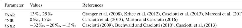
Table 3.Isotope effect cases.
Parameter Values References
εNAR 13 ‰, 25 ‰ Granger et al. (2008), Kritee et al. (2012), Casciotti et al. (2013), Marconi et al. (2017) εNIR 0 ‰ , 15 ‰ Casciotti et al. (2013), Martin and Casciotti (2016)
εNXR −32 ‰,−20 ‰,−13 ‰ Casciotti (2009), Buchwald and Casciotti (2010), Casciotti et al. (2013)
all remineralized DON must be routed either through AMO or AMX, this simplifies the mass balance and ensures that all remineralized14N and15N is accounted for.15NO−2 is re-moved with the isotope effects of NO−2 reduction (αAMX,NIR)
and NO−2 oxidation (αAMX,NXR) in the expected 1:0.3
pro-portion (Brunner et al., 2013). 2.5 Model inversion
Once our N cycle equations were set up as described above, we input them into MATLAB in block matrix form. The equations were of the general formAx=b. All model ocean boxes (200 160 in total) are accounted for in the matrices. Matrix A(400 320×400 320) contained the rate constants and other parameters that are multiplied by the vector of state variables,x(400 320×1). Vectorxcontained the state vari-ables (i.e., [NO−3] and [NO−2] or [DON] and [PON]) to be solved for by the linear solver. Vectorb(400 320×1) con-tained the rates that were independent of the state variables, such as N2fixation and N deposition. Let us consider, as an
example, the DIN model setup. The top left corner of matrix A would contain rate constants for processes that produce and consume NO−3 that are also dependent on [NO−3]. The top right corner of matrixAwould contain rate constants for processes that produce and consume NO−3 but are dependent on [NO−2]. The bottom left corner of matrixAwould con-tain rate constants for processes that produce and consume NO−2 but are dependent on [NO−3]. The bottom right corner of matrix Awould contain rate constants that produce and consume NO−2 and are also dependent on [NO−2]. The top half of vectorxwould be [NO−3] for each model box, and the bottom half of vectorxwould be [NO−2] for each model box. The top half of vectorbwould be independent processes that produce or consume [NO−3], and the bottom half of vector bwould be independent processes that produce or consume [NO−2].
In MATLAB, we used METIS ordering, which is part of the SuiteSparse (http://faculty.cse.tamu.edu/davis/ suitesparse.html, last access: December 2017) to order our large, sparse matrix A. We then used the built-in function “umfpack” with METIS to factorize matrixA. The built-in matrix solver “mldivide” was then used with the factorized components of matrixAand matrixbto solve forx.
2.6 Parameter optimization
There are many parameters in the model that control the rates of the different N cycle processes (Tables 1–3). Some of these parameters are well constrained by literature values (Table 1). Others, such as the rate constants, were objects of our investigation and were optimized against available observations (Table 2). For our optimization, we compared model output using different parameter values to a database of NO−3 and NO−2 concentrations and isotopes. The database was originally compiled by Rafter et al. (2019) and has been expanded to include some additional unpublished data (Ta-ble S2). All of the database observations were binned and interpolated to the model grid. If multiple observations oc-curred within the same model grid box, the values were aver-aged and a standard deviation was calculated. The database was divided randomly into a training set, used for optimiza-tion, and a test set, used to assess model performance. The same number of grid points with observations was used in the training and test sets.
The optimization procedure used the MATLAB function “fminunc” to obtain values for the nonfixed parameters that minimized a cost function (Eq. 22). In each iteration of the optimization, the model system was solved by running the 14N-organic N model,15N-organic N model, 14N-DIN model, and 15N-DIN model. The modeled output [NO−3], [NO−2], δ15NNO3, and δ
15N
NO2 were compared to values
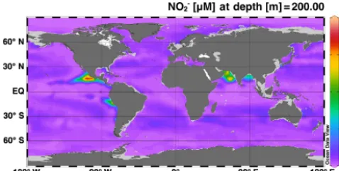
Figure 2.Map showing the model-estimated accumulation of nitrite (NO−2) at 200 m depth.
Cost= wNO3 nNO3sdNO3
X
([NO−3]model− [NO−3]training)2
+ wNO2 nNO2sdNO2
X
([NO−2]model− [NO−2]training)2
+ wδNO3 nδNO3sdδNO3
X
(δ15NNO3,model−δ
15N
NO3,training)
2
+ wδNO2 nδNO2sdδNO2
X
(δ15NNO2,model−δ
15N
NO2,training)
2. (22)
Thewterms are weighting terms introduced to scale the con-tributions of the four observed parameters to equalize their contributions to the cost function. Thenterms and standard deviation (sd) terms were used to normalize the contributions of each measurement type to the cost function. Eachnterm is equal to the number of each type of measurement in the train-ing dataset (e.g., the number of [NO−3] data points=nNO3).
The sd term is equal to the standard deviation of all the mea-surements of a given type (e.g., the standard deviation of all the [NO−3] data points within the training set).
In order to account for error in our model parameter esti-mates, we also iterated over several possible values for three of the most important isotope effects for processes in ODZs: εNAR,εNIR, and εNXR (Table 3). We chose to iterate over
these parameters rather than optimize them since there is a large range of estimates for each of these parameters. We as-signed different possible values for each of these parameters (Table 3), resulting in 12 possible combinations. The opti-mization protocol was performed for each of those combi-nations and unique optimized parameter sets were obtained. The parameter results were then averaged (final values, ble 2) and their spread is categorized as the error (error, Ta-ble 2).
3 Results
3.1 Global model–data comparison
The simulations of NO−2 concentration and isotopic compo-sition are the most unique features of this model in
compari-son to existing global models of the marine N cycle. As such, NO−2 accumulation in ODZs is a feature that should be well represented by the model in order to use it to test hypothe-ses about proceshypothe-ses that control N cycling and loss in ODZs. Overall, we see NO−2 accumulating at 200 m in the major ODZs of the Eastern Tropical North Pacific (ETNP), East-ern Tropical South Pacific (ETSP), and the Arabian Sea (AS) (Fig. 2), which is consistent with observations and expected based on the low O2conditions found there. However,
ac-cumulation of NO−2 in the model ETSP was lower than ex-pected. The model also accumulated NO−2 in the Bay of Ben-gal, which is a low-O2region off the east coast of India that
does not generally accumulate NO−2 or support water column denitrification, but is thought to be near the “tipping point” for allowing N loss to occur (Bristow et al., 2017). Possi-ble reasons for the underestimation of NO−2 in the ETSP and overestimation in the Bay of Bengal will be discussed further in Sect. 4.2.
The model optimization described above yielded a set of isotope effects that best fit the global dataset of [NO−3], [NO−2], δ15NNO3 and δ
15N
NO2. The best fit was achieved
for isotope effects of 13 ‰ for NO−3 reduction (εNAR), 0 ‰
for NO−2 reduction (εNIR), and−13 ‰ for NO−2 oxidation
(εNXR). Figure 3 shows the test set comparison for the global
best-fit set of isotope effects overlaid with a 1:1 line, which the data would follow if there was perfect agreement between model results and observations. There is general agreement between model and observations, with most of the data clus-tering near the 1:1 lines. Agreement between the observa-tions and the training data are similar (Fig. S4), indicating that we did not overfit the training data.
In the test set, there were some low [O2] points where our
model [NO−3] exceeded observations (Fig. 3a, filled black circles); these are largely within the ETSP. In contrast, the AS tended to show slightly lower modeled [NO−3] than ex-pected. The [NO−2] accumulation (Fig. 3b) andδ15NNO3
sig-nals (Fig. 3c) in the ETSP were also generally too low com-pared with observations. These signals are likely tied to in-sufficient NO−3 reduction occurring in the model ETSP. An-other consideration is that there may be a mismatch in resolu-tion between the model and the time and space scales needed to resolve the high NO−2 accumulations observed sporadi-cally (Anderson et al., 1982; Codispoti et al., 1985, 1986).
Overall, the representation of δ15NNO3 was fairly good
(RMSE=2.4 ‰), though there were a subset of points above δ15NNO3=10 ‰ where the modeledδ
15N
NO3 exceeded the
observedδ15NNO3, and others where modeledδ
15N NO3 was
lower than observations (Fig. 3c). Many of the points with overestimated δ15NNO3 were located within the AS ODZ,
where there may be too much NO−3 reduction occurring, leading to artificially elevatedδ15NNO3 values. As indicated
above, the underestimatedδ15NNO3 points largely fell within
the ETSP where we believe the model is underestimating NO−3 reduction. The representation of δ15NNO2 was also
Figure 3. Modeled (a) [NO−3], (b) [NO−2], (c) δ15NNO3, and
(d)δ15NNO2 are compared against the corresponding values from
the database test set. Shown on each panel is a 1:1 line starting at the origin. Data in black have corresponding[O2]<10 µM, and data in gray have[O2] ≥10 µM.
was generally not low enough (Fig. 3d), indicating an under-estimated sink of “heavy” NO−2.
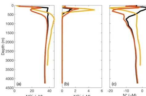
3.2 ODZ model–data comparison using station profiles To further investigate the distribution of model N species within the three main ODZs, we selected representative off-shore grid boxes within each ODZ that contained observa-tions to directly compare with model results in station pro-files. Overall, the modeled NO−3 and NO−2 concentration and isotope profiles in the AS and ETNP were consistent with the observations, with [NO−3] slightly underestimated in the AS ODZ and overestimated in the ETSP (Fig. 4). As [O2] goes to
zero, the O2-intolerant processes NAR, NIR, and AMX are
released from inhibition. These processes result in a decrease in [NO−3] (via NAR) which corresponds to an increase in δ15NNO3, since NAR has a normal isotope effect. NO
− 2 also
starts to accumulate in the secondary NO−2 maximum as a re-sult of NAR. Theδ15NNO2is lower thanδ
15N
NO3 since light
NO−2 is preferentially created via NAR, and this fractiona-tion is further reinforced by the inverse isotope effect of NXR (Casciotti, 2009). These patterns are readily observed in the AS and ETNP, but were less apparent in the ETSP, where [NO−3] depletion and [NO−2] accumulation in the model were lower than observed. This could be due in part to the time-independent nature of this steady-state inverse model, which
Figure 4.Depth profiles comparing model results with binned and averaged database observations from a model water column. Re-sults are shown for offshore regions of the three main oxygen defi-cient zones (ODZs): the Arabian Sea (AS;a–e), the Eastern Trop-ical North Pacific (ETNP;f–j), and the Eastern Tropical South Pa-cific (ETSP;k–o). Average modeled nitrate concentration ([NO−3]), nitrite concentration ([NO−2]), and N∗are shown in black. Gray er-ror lines around the black line show the 2σ spread from the average from the 12 different optimized model results using the different combinations of isotope effects for nitrate reduction (εNAR), nitrite reduction (εNIR), and nitrite oxidation (εNXR). Observed data are shown in yellow in all panels. Modeledδ15NNO3andδ15NNO2 are shown for three different combinations of isotope effect. The blue lines representεNAR=13,εNXR= −13, andεNIR=0, which are the best fit isotope effects globally and in the ETSP. The red lines representεNAR=13,εNXR= −32, andεNIR=0, which are the best fit isotope effects in the AS.
does not capture the effects of upwelling events in the ETSP on N supply and cycling (Canfield, 2006; Chavez and Mes-sié, 2009).
In order to gauge the model results for N loss, we also calculated N∗, a measure of the availability of DIN rela-tive to PO3−4 compared to Redfield ratio stoichiometry (N∗= [NO−3]+[NO−2]−16·[PO3−4 ]; Deutsch et al., 2001). Negative N∗values are associated with N loss due to AMX or NIR or release of PO3−4 from anoxic sediments (Noffke et al., 2012), while positive N∗values are associated with input of new N through N2fixation (Gruber and Sarmiento, 1997). Although
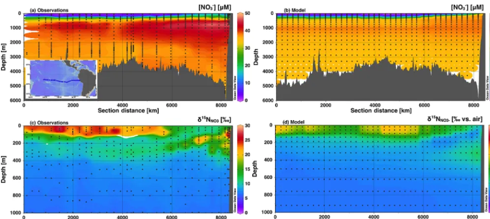
[image:12.612.309.548.67.344.2]Figure 5.Section profiles of NO−3 concentrations and isotopes over the GEOTRACES GP16 cruise track (panelainset) in the South Pacific. Section distance runs from west to east in each panel. Comparison of(a)observed [NO−3] to(b) modeled [NO−3] is presented over the full depth range (0–6000 m). Comparison of(c)observedδ15NNO3 to(d)modeled δ15NNO3 is presented over a shortened depth range (0–1000 m) to better assess surface and ODZ values. GEOTRACES data are from Peters et al. (2018a) and available from Biological and Chemical Oceanography Data Management Office (BCO-DMO).
[NO−2] together with World Ocean Atlas PO3−4 data inter-polated to the model grid to calculate N∗resulting from the model. Both the AS and ETNP showed a decrease in model N∗in the ODZ, as expected for water column N loss. Below the ODZ, N∗increased again and returned to expected deep water values. Modeled N∗in the ETSP, however, did not fol-low the observed trend, consistent with an underestimate of N loss in the model ETSP.
Though the global best fit isotope effects for NAR, NIR, and NXR produced good agreement to the data in general, the isotope effects that best fit individual ODZ regions dif-fered when the cost function was restricted to observations from a given ODZ. For the ETSP, the best fit isotope effects were the same as the previously stated global best fit. For the AS, the best fit isotope effects were εNAR=13 ‰, εNIR=
0 ‰, and εNXR= −32 ‰. For the ETNP, the best fit
iso-tope effects were εNAR=13 ‰, εNIR=15 ‰, andεNXR=
−32 ‰, though the performance is only marginally better than with εNIR=0 ‰. The lower (more inverse) value for
εNXRresulted in higherδ15NNO3 and lowerδ
15N
NO2, which
better fit the ODZδ15NNO2 data compared to the global best
fit εNXR= −13 ‰. These results are consistent with earlier
isotope modeling studies in the ETSP (Casciotti et al., 2013; Peters et al., 2016, 2018b) and in the AS (Martin and Cas-ciotti, 2017). Although, in the AS, modeledδ15NNO3 values
were too high, likely in part due to overpredicted rates of NAR, which also resulted in lower modeled [NO−3] (Fig. 4).
3.3 Model–data comparison in GEOTRACES sections We also investigated the agreement between global best fit model concentration and isotope distributions with data from two GEOTRACES cruise sections: GP16 in the South Pa-cific, and GA03 in the North Atlantic. For GP16, we see that [NO−3] is low in surface waters and increases to a mid-depth maximum between 1000 and 2000 m. The highest [NO−3] are found at mid-depth in the eastern boundary of the section. The model reproduces the general patterns, matching obser-vations fairly well in the surface waters, but diverges below 500 m (Fig. 5). Although the patterns are generally correct, insufficient NO−3 is accumulated in the deep waters of the model Pacific. This could be due to an underestimate of pre-formed NO−3 (over estimate of assimilation in the Southern Ocean), or inadequate supply of organic matter to be rem-ineralized at depth. In the Southern Ocean, model surface [NO−3] are 5–10 µM lower than observations (Fig. S5), which could be enough to explain the lower-than-expected [NO−3] in the deep Pacific, which is largely sourced from the South-ern Ocean (Rafter et al., 2013; Sigman et al., 2009; Peters et al., 2018a, b).
In the GP16 section, we also see that there are elevated δ15NNO3 values in the model surface waters and in the ETSP
ODZ (Fig. 5d), as expected from observations (Fig. 5c). However, we can also see that the insufficient depletion of NO−3 and increase inδ15NNO3 in the ETSP ODZ (Fig. 5b
ETSP ODZ and the upper thermocline in the eastern part of the section is consistent with an underestimate of NO−3 re-duction. In GP16 we were also able to compare modeled and observed [NO−2] and δ15NNO2 (Fig. S6). Patterns of
mod-eled [NO−2] andδ15NNO2 showed accumulation of NO
− 2 in
the ODZ, with an appropriate δ15NNO2 value (Fig. S6).
Al-though, generally lower modeled concentrations of NO−2 in the ODZ also support an underestimate of NAR (Fig. S6).
Surfaceδ15NNO3 values were also not as high in the model
as in the observations (Fig. 5), which could result from insuf-ficient NO−3 assimilation or too low suppliedδ15NNO3
(Pe-ters et al., 2018a). However, we do see a similar depth range for high surfaceδ15NNO3and a localδ
15N
NO3 minimum
be-tween the surface and ODZ propagating westward in both the model and observations, indicating that the physical and bio-geochemical processes affectingδ15NNO3 are represented by
the model. Additionally, the model shows slightly elevated δ15NNO3 in the thermocline depths (200–500 m) west of the
ODZ, which is consistent with the observations (Fig. 5c), though not of the correct magnitude. This is partly related to the muted ODZ signal as mentioned above and its lessened impact on thermocline δ15NNO3 across the basin. Peters et
al. (2018a) and Rafter et al. (2013) also postulated that these elevatedδ15NNO3values were in part driven by
remineraliza-tion of organic matter with highδ15N. Theδ15N of sinking PON in the model (6 ‰–10 ‰) was similar to those observed in the South Pacific (Raimbault et al., 2008), as well as those predicted from aforementioned N isotope studies (Rafter et al., 2013; Peters et al., 2018a). The model also shows slightly elevatedδ15NNO3 in the intermediate depths (500–1500 m),
which is consistent with observations, again reflecting rem-ineralization of PON with δ15N greater than mean ocean δ15NNO3. Overall, the patterns of δ
15N
NO3 for the model
GP16 are correct but the magnitudes of isotopic variation are muted, largely due to the lack of N loss in the ODZ and modeled surface δ15NNO3 values that are lower than
obser-vations. The simplification of NH+4 dynamics in the model could also contribute to underestimation ofδ15NNO3values if
there was a large flux of15N-enriched NH+4 from sediments (Granger et al., 2011), or if15N-depleted NH+4 was preferen-tially transferred to the N2pool via anammox. While the
iso-tope effect on NH+4 during anammox (Brunner et al., 2013) is indeed higher than that applied here, we chose to balance this with a low isotope effect during aerobic NH+4 oxidation (Table 1).
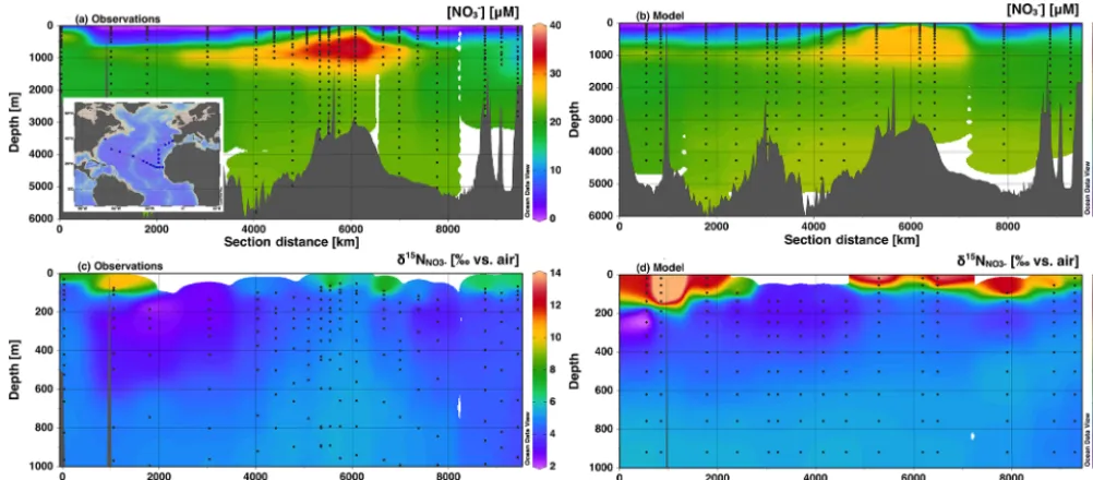
In the North Atlantic along GEOTRACES section GA03, we see good agreement between the observed and mod-eled [NO−3] (Fig. 6). There is generally low surface [NO−3] with a distinct area of high [NO−3] propagating from near the African coast. Deep water (>2000 m) [NO−3] is lower than we see in the Pacific section, and the model matches well with the Atlantic observations. Again, there is not quite enough NO−3 present in Southern Ocean-sourced interme-diate waters (500–1500 m; Marconi et al., 2015). Modeled δ15NNO3 values at first glance appear higher than observed
values at the surface (Fig. 6). However, many of the surface [NO−3] were below the operating limit for δ15NNO3
analy-sis and were not determined. Focusing on areas where both measurements and model results are present yields excellent agreement. For example, we do see lowδ15NNO3 values in
upper thermocline waters in both the model and observa-tions, likely corresponding to lowδ15N contributions from N2fixation that is remineralized at depth and accumulated in
North Atlantic Central Water (Marconi et al., 2015; Knapp et al., 2008). The model input includes significant rates of N2fixation in the North Atlantic that are consistent with this
observation (Fig. S1). However, rates of N deposition in the North Atlantic are also fairly high and can contribute to the lowδ15N signal (Knapp et al., 2008). In our model, atmo-spheric N deposition contributed between 0 % and 50 % of N input along the cruise track.
4 Discussion
4.1 Assumption checks
As previously mentioned (Sect. 2.3), organic N and DIN were modeled separately in order to introduce dependence on both organic N and substrate availability for the heterotrophic processes NAR and NIR. These separate model runs required several assumptions to be made regarding the processes that impact both organic N and DIN, namely assimilation and remineralization.
mod-Figure 6.Section profiles of NO−3 concentrations and isotopes over the GA03 cruise track (panelainset) in the North Atlantic. In each panel, section distance runs from west to east for the first 6000 km, and then runs from south to north. Comparison of(a)observed [NO−3] to
(b)modeled [NO−3] is presented over the full depth range (0–6000 m). Comparison of(c)observedδ15NNO3to(d)modeledδ
15N
NO3is
pre-sented over a shortened depth range (0–1000 m) to better assess surface and the lowδ15NNO3contribution from N2fixation. GEOTRACES
data are from Marconi et al. (2015) and available from BCO-DMO.
eled [NO−3] that was higher than observed [NO−3] (Fig. S7). Likewise, points with relatively lower DIN assimilation had modeled [NO−3] less than observed [NO−3]. However, the ma-jority of DIN assimilation estimates were within 10 µM yr−1 of the organic N production estimates, with an average off-set of approximately 3.5 % compared to DIN assimilation. The total global assimilation rates were within 0.4 %, with some spatially variable differences due to offset between sur-face [NO−3] and modeled [NO−3]. However, we find that the World Ocean Atlas surface NO−3 values are fairly well repre-sented by our modeled surface NO−3 (Fig. S5). We conclude that though the assimilation rates are not identical in the or-ganic N and DIN model runs, the discrepancy in modeled DIN assimilation is less than 0.1 %, and there is unlikely to be significant creation or loss of N as a result of the split model.
4.2 Model dependency on input O2
The modeled concentration and isotope profiles for the ETSP, unlike in the AS and ETNP, reflected an underestimation of water column denitrification in the best-fit model. In ETSP measurements, there is a clear deficit in [NO−3], coinci-dent with the secondary NO−2 maximum and N∗ minimum (Fig. 4). In our modeled profiles, this NO−3 deficit is miss-ing, and although a secondary NO−2 maximum is present, its magnitude is lower than observed (Fig. 4). The model also does not capture the negative N∗ excursion (Fig. 4), which we think reflects a model underestimation of NAR and
NIR in the ETSP. The cause of this missing denitrification is likely to be poor representation of the ETSP O2 conditions
in the model grid space. Since our model grid is fairly coarse (2◦×2◦), only a few boxes within the ETSP had averaged [O2] below the thresholds that would allow processes such as
NAR and NIR to occur. The anoxic region of the ETSP is ad-jacent to the coast and not as spatially extensive as in the AS and ETNP (Fig. S8); therefore, this region in particular was less compatible with the model grid. In order to test whether the parameterization of O2dependence was the cause of the
low N loss, we ran the model using the globally optimized parameters (Table 3) but with higher O2thresholds (15 µM)
for NAR, NIR, and AMX (Table 1). This extended the re-gion over which ODZ processes could occur and resulted in an increase in water column N loss from 6 to 32 Tg N yr−1in the ETSP, which is more consistent with previous estimates (DeVries et al., 2012; Deutsch et al., 2001). This change also stimulated the development of a NO−3 deficit, larger sec-ondary NO−2 maximum, and N∗ minimum within the ODZ (Fig. 7).
As previously mentioned (Sect. 3.1), modeled [NO−2] in the Bay of Bengal is higher than observations. The accumu-lation of NO−2 here in the model is likely due to O2
[image:15.612.47.548.67.287.2]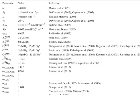
![Figure 3. Modeleddata in gray have (a) [NO−3 ], (b) [NO−2 ], (c) δ15NNO3, and(d) δ15NNO2 are compared against the corresponding values fromthe database test set](https://thumb-us.123doks.com/thumbv2/123dok_us/8144477.245857/12.612.309.548.67.344/figure-modeleddata-gray-compared-corresponding-values-fromthe-database.webp)