Automatic Ice Surface and Bottom Boundaries Estimation in Radar Imagery Based on Level Set Approach

Automatic Ice Surface and Bottom

Boundaries Estimation in Radar Imagery

Based on Level Set Approach

Maryam Rahnemoonfar

,

Member, IEEE,

Geoffrey C. Fox

, Masoud Yari

, John Paden

Abstract—Accelerated loss of ice from Greenland and Antarctica has been observed in recent decades. The melting of polar ice sheets and mountain glaciers has a considerable influence on sea level rise in a changing climate. Ice thickness is a key factor in making predictions about the future of massive ice reservoirs. The ice thickness can be estimated by calculating the exact location of the ice surface and sub-glacial topography beneath the ice in radar imagery. Identifying the locations of ice surface and bottom is typically performed manually which is a very time consuming procedure. Here we propose an approach which automatically detects ice surface and bottom boundaries using distance regularized level set evolution. In this approach the complex topology of ice surface and bottom boundary layers can be detected simultaneously by evolving an initial curve in the radar imagery. Using a distance regularized term, the regularity of the level set function is intrinsically maintained which solves the reinitialization issues arising from conventional level set approaches. The results are evaluated on a large dataset of airborne radar imagery collected during IceBridge mission over Antarctica and Greenland and show promising results with respect to manually picked data.

I. INTRODUCTION

In recent years global warming has caused severe threats to our environment. Accelerated loss of ice from Greenland and Antarctica has been observed

1. Department of Computing Sciences, Texas A&M University-Corpus Christi, Corpus Christi, TX

2. School of Informatics and Computing, Indiana University, Bloomington, IN

3. Department of Engineering, Texas A&M University-Corpus Christi, Corpus Christi, TX

4. Center for Remote Sensing of Ice Sheets, University of Kansas, Lawrence, KS

* Corresponding Author

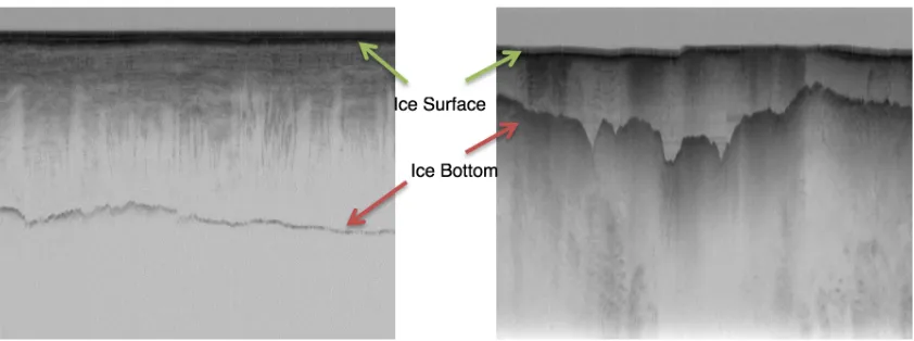
sub-glacial topography. The sub-glacial topography hidden beneath the thick ice sheets can take any shape from smooth to mountainous (Figure 1).

For ice surface and bottom identification, usually manual (human) picking of radargrams is taken. Manual boundary identification is a very time con-suming and tedious task which can introduce errors. As radar data volumes continue to increase and to improve the reliability of boundary identification, we seek to develop automatic techniques for this process.

There are several challenges in automatic pro-cessing of ice surface and bottom layers. These challenges can be split into three categories. The first is that the ice bottom may suffer from low signal to interference and noise ratios (SINR). Low SINR is caused by several factors: a) signal attenuation while traveling through ice, b) radar clutter energy, and c) thermal noise and occasional electromagnetic interference. The second is that the subglacial topography is highly variable on a continental scale ranging from flat to mountainous. Finally, artifacts in the data, such has surface mul-tiples (ringing of the radar signal between the large metal aircraft and the ice surface), can lead to false identification of the ice bottom layer.

In this paper, we propose an automatic technique which can overcome most of the aforementioned challenges. Here we propose a novel level set ap-proach to automatically identify the ice surface and bottom layers in a large dataset of radar imagery. In this approach, using an initial curve, the image will be divided into two parts: inside the curve and outside the curve. In the next step, by help of external and internal forces, each point on the curve starts moving at a variable speed and the curves will gradually evolve until all boundaries are detected. In the conventional level set formulation, the level set function typically develops irregularities during its evolution and needs re-initialization to periodically replace the degraded level-set function. Here we used a variational level set function in which the regularity of the level set function is maintained intrinsically.

After this introduction, the related works will be discussed in section 2. The details of the proposed

method will be discussed in section 3. Experimental results will be discussed in section 4. The results are evaluated in section 5. Section 6 highlights the conclusions of this work.

II. RELATED WORKS

Research on subsurface imaging (including seis-mic methods) is too vast to review here; see Turk et al [5] for an extensive review. Several semi-automated and semi-automated methods have been in-troduced in the literature for layer finding and ice thickness in radar images [6], [7], [8], [9], [10], [11], [12], [13], [14], [15], [16], [17], [18], [19], [20]. Freeman et al. [9] finds near surface ice layers in images from the shallow subsurface radar on NASA’s Mars reconnaissance Orbiter (SHARAD). First the layers were transformed to horizontal layers and then several filtering and thresholding techniques were applied to enhance the image and discard unclear layers. Finally the layers were trans-formed back to image space. Our algorithm is quite distinct from this method in the sense that it does not need any intermediate thresholding which might be different from one image to another. Ferro & Bruzzone [8] proposed an algorithm to extract the deepest scattering area visible in radargrams from the SHARAD mission acquired on the north polar layered deposits of Mars. Their algorithm is based on discriminating the statistical properties of subsurface targets and finding a suitable fitting model. This method is unable to find exact layers in the ice and only provides approximate locations of different sub-regions based merely on the statistical analysis of the signal.

Fig. 1. Ice surface and bottom depicted in radar echograms gathered by the Multichannel Coherent Radar Depth.

Gibbs sampling instead of dynamic programming based solver was used for performing inference. The problem with using graphical models is that it needs a lot of training samples (around half of the actual dataset) which are ground-truth images labeled manually by a human. Given the fact that manual ice layer detection is a very time consuming and expensive task, the last three methods are not practical for large datasets.

In another work, Gifford et al. [11] compared the performance of two methods, edge based and active contour, for automating the task of estimating polar ice and bedrock layers from airborne radar data acquired over Greenland and Antarctica. They showed that their edge-based approach offers faster processing but suffers from lack of continuity and smoothness that active contour provides. In their active contour approach, the contour’s shape is adaptively modified and evaluated to minimize the cost or energy in the image [21], [22]. The main disadvantage of the active contour model is the incapability of maintaining the topology of the evolving curve. This difficulty does not arise in the level set model as it embeds the evolving curve into a higher dimensional surface. Mitchell et al. [15] used a level set technique for estimating bedrock and surface layers. However for each single image the user needs to re-initialize the curve manually and as a result the method is quite slow and was

applied only to a small dataset. In this paper, the regularity of level set is intrinsically maintained using a distance regularization term. Therefore it does not need any manual re-initialization and was automatically applied on a large dataset.

III. METHODOLOGY

Here we propose to use level sets technique to precisely detect the ice surface and the bottom boundary. The level set method (LSM) is essentially a successor to the active contour method. Ac-tive contour method (ACM), also known as Snake Model, was first introduced by Kass et al. [22]. The ACM is designed to detect interfaces and bound-aries by a set of parametrized curves (contours) that march successively toward the desired object until the desired interfaces are captured. Assume these parametrized curves are expressed as

C(s, t) = (x(s, t), y(s, t)) s∈[0,1], t∈[0,∞) (1) where s is the parameter of the curve length and

image, so that it can eventually lead the front curve to the boundaries of the desired object.

Therefore, the front curve C(s, t) moves and should eventually capture the interface of the de-sired object according to the following differential equation

∂C

∂t =F N (2)

where F is the velocity function for the mov-ing curve C and N determines the direction of the motion. Here N is the normal vector to the curve C. Even though the ACM is an efficient tool in image and video segmentation, it suffers from certain serious issues. Being a parametrized approach, the ACM approach can fail, because it is incapable of consistently handling the topology of the front moving curve. In fact, in each iter-ation, certain parts of the curve C can split or merge since leading reference points can distance from or come closer to each other; therefore, the topology of the front curve can undergo substantial changes in each iteration. The accumulation of such changes of topology can introduce unnecessary, or even misleading, complexities to the process, which will cause the frontier curve to fail in tracking the right interface in the image. To overcome the disadvantages that the snakes model presents, the level set method (LSM) was proposed by Osher and Sethian [23]. Rather than following the interface itself as in ACM, the level set method takes the original curve and builds it into a surface. In other words, the LSM takes the problem to one degree higher in the spatial dimension (Figure ??) and considers the curve C(s, t) as the zero-level of a surface z = ϕ(x, y, t) at any given time t. The function ϕ is called the level set function (LSF). We then track the changes of C(s, t) as the three dimensional shape,ϕevolves at each iteration.

More precisely, assume the curveC(s, t) is the interface of an open region Ωt ⊂ R2_{. We embed}

the curve C(s, t) in the surface z = ϕ(x, y, t) in a way thatC(s, t)will be the zero level set of the LSF,ϕ, which takes negative values insideΩtand

positive values outside of it; that is

ϕ(x, y, t) = 0 forx∈∂Ωt, (3)

and

ϕ(x, y, t)<0for ∈Ωt,

ϕ(x, y, t)>0for ∈/Ω¯t.

(4)

The advantage of the LSM is that it handles changes in the topology organically and does not create any unnecessary complexity. However, this comes with a higher computational price: instead of a 2D curve, as in ACM, we are now moving a 3D object in each iteration. But as mentioned, we should only track the zero level set of the surfaceϕ. Therefore, it makes sense to evolve only a narrow band around the zero-level set to reduce the computational cost. In fact, this method has been proposed by the same authors in their later works. We will also take advantage of this computational shortcut as we proceed.

In the setting of the level set method, the LSF,ϕ, is the solution of the following dynamical system

∂ϕ ∂t =−

∂F

∂ϕ (x, y, t)∈Ω×[0,∞] (5)

with a typical initial condition. In Eq. 5, F rep-resents the level set functional; conventionally, in image segmentation approaches, the functional F is defined as the ensemble of several forces, such as the edge and the area forces:

F =Eedge+Earea (6)

where

Eedge(ϕ) =λ Z

Ω

gδ(ϕ)|∇ϕ|dx (7)

Earea(ϕ) =α Z

Ω

gH(−ϕ)dx (8)

indicator on Ω, the area of the image, which is defined by

g= 1

1 +|∇Gσ∗I|

2 (9)

whereIis the image intensity andGσis a Gaussian kernel with a standard deviationσ.

The edge term, Eedge computes the line inte-gral along the zero level contour of ϕ; that is,

R1

0 g(C(s))|C

0_{(s)|ds, where the curve C=C(s) :}

[0,1] → Ω is the zero-level contour and s is the curve length. This term will be minimized whenC

is positioned on the boundary of the desired object. The area term, Earea, is basically calculated as a weighted area of the region inside the zero level contour. It accelerates the motion of the zero-level contours toward the desired object.

Therefore, to minimize the energy functional,F, it is necessary to solve the following PDE system:

∂ϕ

∂t =λδ(ϕ)div

g_|∇∇ϕ_ϕ|+αgδ(ϕ);

ϕ(x,0) =ϕ0(x); (x, t)∈Ω×[0,∞).

(10) This system is subject to the no-flux boundary conditions on Ω, which signifies that there is no external force outside the image area. To carry out a numerical process to solve this PDE system, the spatial derivatives are discretized using the upwind scheme. The use of the central difference scheme will result in instability in the numerical procedure. The numerical procedure also involves the assump-tion that |∇ϕ| = 1. We initialize the procedure with a function that satisfies this property, but the numerical scheme will not pass on this property; consequently at each step an extra care, known as re-initialization, must be taken to avoid the error accumulation. The reinitialization procedure involves solving the following PDE system for ψ

in each step

∂ψ

∂t =sign(ϕ)(1− |∇ψ|). (11)

This severely slows down the computation. To overcome this difficulty we use the distance reg-ularized level set evolution (DRLSE) method as

proposed in [24] — also see [21] . In the DRLSE method, the level set functional F is defined as

F=Eedge+Earea+Ep, (12)

whereEprepresents the distance regularization term defined by

Ep(ϕ) =µ Z

Ω

p|∇ϕ|dx, (13)

with a potential functionpand a constantµ >0. As suggested in [24] , we use a double-well function for the potential function pas follows

p(s) =

_{(1−cos(2πs))/4π}2 _s≤1,

(s−1)2/2 s≥1, (14)

withs∈[0,∞).

We have

∂Ep

∂ϕ =−µdiv(D∇ϕ), (15)

where the diffusion coefficientD=D(ϕ)is given by

D(ϕ) =p 0_(|∇ϕ|)

|∇ϕ| . (16)

It is discussed in [24] that p has two minimum points at s = 0 and s = 1; and it is twice differentiable with the following properties

|p 0_(s)

s | <1 fors >0 , and

lim s→0

p0(s)

s = lims→∞

p0(s)

s = 1. (17)

Given the above properties, one can easily see that

|µp

0_(|∇ϕ|)

|∇ϕ| | ≤µ. (18)

That means the diffusion coefficient in (15) remains bounded. Now the new energy functionalF can be minimized by solving the following gradient flow:

∂ϕ

∂t =λδ(ϕ)div

g_|∇∇ϕ_ϕ|+αgδ(ϕ) +µdiv(D∇ϕ), ϕ(x,0) =ϕ0(x),

(x, t)∈Ω×[0,∞).

Thanks to the distance regularization term, the central difference scheme can be used to discretize spatial derivatives, which leads to a stable numerical procedure without need of re-initialization .

It also must be noted that, in practice, the func-tions δ and H are approximated by the smooth functionsδε andHε defined by

δε(x) =

1

2ε 1 + cos πx

ε

|x| ≤ε,

0 |x|> ε; (20)

and

Hε(x) =

  

1 2 1 +

x ε+

1

πsin πx

ε

|x| ≤ε,

1 0

|x|> ε,

|x|<−ε; (21) forε >0.εis often considered to be 3/2.

As mentioned before, the above equation is gov-erned by the no-flux boundary condition. For the initial condition, we will consider a simple step function defined by

ϕ0=

−c0 x∈Ω0,

c0 x∈Ω/Ω0;

(22)

where c0 > 0 is a constant, and Ω0 is a region

inside the image regionΩ.

IV. EXPERIMENTAL RESULTS

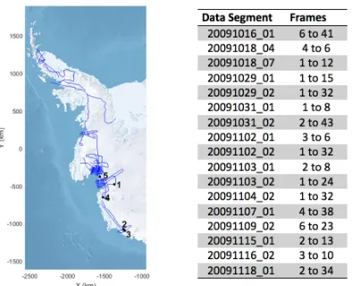
We tested our ice layer identification approach on publicly available radar images from the 2009 NASA Operation IceBridge Mission. The images were collected with the airborne Multichannel Co-herent Radar Depth Sounder system described in [2]. The images have a resolution of 900 pixels in the horizontal direction, which covers around 50km on the ground, and 700 pixels in the vertical direc-tion, which corresponds to 0 to 4km of ice thick-ness. For these images there are manually picked in-terfaces and we compare our ice layer identification approach with them. The manually picked interfaces have been produced by human annotators and some of them are inaccurate and contain only one layer. We chose the images that have both ice surface and bottom layers and tested our method on a total of 323 images. Figure 2 shows the corresponding map and data segments of our entire dataset from

Fig. 2. The map and data segments of our dataset, 1) Fig. 1 right, frame ID 2009110202008, 2) Fig. 3, frame ID 2009101601021, 3) Fig. 4, Fig. 1 left, frame ID 2009101601026, 4) Fig. 5, frame ID 2009110202023, 5) Fig. 6, frame ID 2009110202032

CReSIS website (https://data.cresis.ku.edu/data/rds/ ). Since our method is fully automatic we do not need any training dataset and our method is not affected by inaccurate ground-truth. Moreover human annotation is quite time consuming and because our method does not need any training and is independent of ground-truthing, it is quite fast. We used the same iteration number of 800 for all of the images.

Figure 3 through 6 show the results of our approach with respect to the manually picked in-terfaces in a diverse dataset which includes images with clutter from englacial scattering, large variabil-ity of sub-glacial topography, surface multiples and faint ice bottoms.

A. Clutter

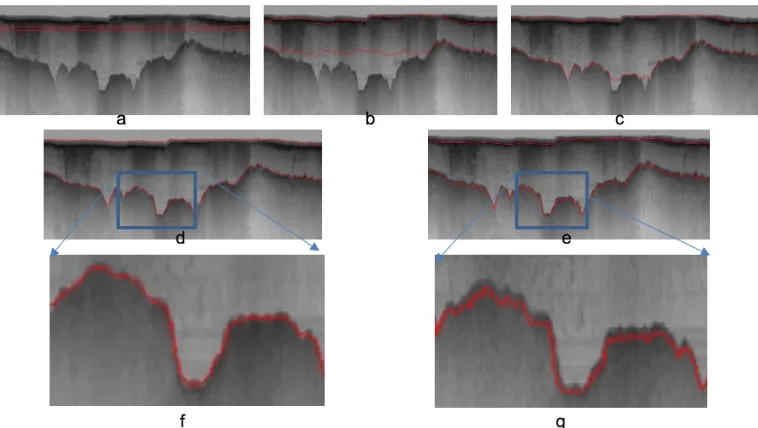
curve. This initial curve was drawn automatically and there is no need for user input in any step of the procedure. Figure 3b-e shows the results after iteration 200, 400, 600, and 800 respectively. As it can be seen in Figure 3b, after 200 iterations the ice surface is approximately detected but the ice bottom is still not detected. After 400 iterations, part of the ice bottom is detected, but after 800 iterations both the ice surface and bottom layers are detected perfectly. Figure 3f shows the manually picked interfaces which is the result of labeling the layers by a human operator. Comparing Figure 3e, the result of the proposed approach, with Figure 3f, the manually picked interfaces, we notice that our result is very close to the manually picked interfaces and appears to be even more accurate in some parts as shown in Figure 3g and Figure 3h. The automated approach removes much of the tedium from the task by providing automated results for most of the ice bottom and allowing the operator to focus on the harder to track regions where the automated algorithm fails.

B. Diverse sub-glacial topology

The subglacial topography can vary from a smooth shape to a very rough topology due to varia-tion in landscape relief. Figure 4 shows an example where the ice bottom is rougher. The same initial curve as the previous example was utilized in Figure 4a. After 400 iterations (Figure 4c), the approximate shape of the ice surface and bottom is detected. After 600 iterations the solution is converged and the exact shape of both layers are detected. Here we continued the iteration to 800 to have the same conditions for all images. As can be seen in Figure 4d, the perfect shapes of the ice surface and bottom are maintained and the extra iterations did not make the situation worse. Comparing our results (Figure 4d) with the manually picked interfaces (Figure 4e), we find our results are more smooth and accurate than the manually picked interfaces. Figure 4f and g show the magnified sections of images in Figure 4d and e.

C. Surface multiple

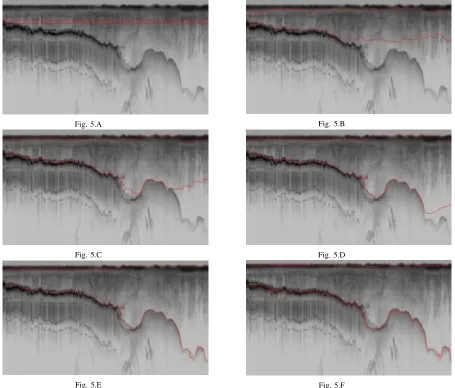
Strong surface reflections can occur due to re-flecting the energy back from the ice sheet surface to the receiver antenna and back to the surface again. The Surface multiple is another challenging factor in processing and identification of the ice surface and bottom. Figure 5 shows an example of a surface multiple with a more complicated shape of ice bottom and with a high level of clutter in the im-age. Here it takes the full 800 iterations for the level set solution to converge, but it shows a satisfactory results compared to the manually picked interfaces. This representative result show the robustness of our algorithm to the surface multiple.

V. EVALUATION

To evaluate the performance of our approach, first we need to set up some benchmarks. For any particular pixel in the image that we are evaluating, there are four cases in comparison with the man-ually picked interfaces (ground-truth); these four cases are true positive (TP) or correct result, false positive (FP) or unexpected result, false negative (FN) or missing results, and finally true negative (TN) [25]. For example, in a radar image, pixels that are located on the interfaces in the ground-truth image and are classified the same by our method are TP. Pixels that are not on any interfaces in the ground-truth image and are not classified in any of them by our method are TN, etc. From the confusion matrix, precision (P) and recall (R) are calculated as follow:

R= T P

T P +F N (23)

P = T P

T P +F P (24)

Precision, the exactness of a classifier, and recall, the completeness of a classifier, can be combined to produce a single metric known as F-measure, which is the weighted harmonic mean of precision and recall. The F-measure defined as:

F = 1

α1_p+ (1−α)_R1 =

β2+ 1P R

Fig. 3. Contour evolution throughout processing. a) Initial curve, (b)-(e) contour adaptation to ice surface and bottom layers after 200, 400, 600, and 800 iterations correspondingly, (f) manually picked interfaces, (g)-(h) the magnified section of (e) and (f)

Fig. 5.A Fig. 5.B

Fig. 5.C Fig. 5.D

Fig. 5.E Fig. 5.F

Fig. 5. Contour evolution throughout processing. Fig 5.A is the initial curve, Fig 5.B-E are contour adaptation to ice surface and bottom after 200, 400, 600, and 800 iterations respectively, Fig 5.F is the manually picked interfaces

captures the precision and recall tradeoff. The F-measure is valued between 0 and 1, where larger values are more desirable. In this paper we used a balanced F-measure, i.e. withβ = 1.

The assumption is that human labeled images (ground-truth) contain perfect results and then the performance of our method was evaluated with respect to manually picked interfaces. We calculated the precision, recall and F-measure for all of the

Fig. 6. Our approach is not able to detect the invisible parts of ice bottom, left: the ice surface and bottom detected by our approach, right: manually picked interfaces

images and reached 75% F-measure for the entire dataset. For the images that have visible ice bottom layers (1/3 of dataset), we reached the average F-measure of 96% (Table I ).

F-measure

Entire dataset (visible and invisible ice bottom) 75%

Images with visible ice bottom 96%

TABLE I. Average F-measure of our approach for the entire dataset and also for the images with visible ice bottom.

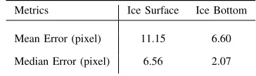
We also calculated the accuracy by computing the mean absolute deviation between the manually picked and the estimated layer boundaries by our algorithm. We used two summary statistics: mean column-wise absolute error over all images in the visible datatset and the median of the column-wise mean absolute errors across images (Table II ).

Metrics Ice Surface Ice Bottom

Mean Error (pixel) 11.15 6.60

Median Error (pixel) 6.56 2.07

TABLE II. Mean and median error on ice surface and bottom

Our algorithm is very fast, taking an average of 30 second to process each image on a 2.7 GHz machine. Moreover it does not need any training

phase with human labeled images which speeds up the entire process significantly. Usually it takes up to 5-10 minutes per file to manually label the image [11].

VI. CONCLUSION AND FUTURE WORK

numbers of iterations. In the future, we are planning to extend this work by improving the quality of the images with faint or currently undetectable ice bottom signals prior to applying the level set algorithm. In future, we will be looking at other dataset especially those with internal ice layers. We will also try to implement the Viterbi method [19], [20] for providing a faster solution in comparing to level-set algorithm.

REFERENCES

[1] A. Shepherdet al., “A reconciled estimate of ice-sheet mass balance (vol 57, pg 88, 2010),”Science, vol. 338, no. 6114, pp. 1539–1539, 2012.

[2] C. Allen, L. Shi, R. Hale, C. Leuschen, J. Paden, B. Pazer, E. Arnold, W. Blake, F. Rodriguez-Morales, and J. Ledford, “Antarctic ice depthsounding radar instrumentation for the nasa dc-8,”Aerospace and Electronic Systems Magazine, IEEE, vol. 27, no. 3, pp. 4–20, 2012.

[3] C. Leuschen, “Icebridge snow radar l1b geolocated radar echo strength profiles,” Boulder, Colorado, NASA DAAC at the National Snow and Ice Data Center, do i, vol. 10, 2013.

[4] S. Gogineni, J.-B. Yan, J. Paden, C. Leuschen, J. Li, F. Rodriguez-Morales, D. Braaten, K. Purdon, Z. Wang, and W. Liu, “Bed topography of jakobshavn isbr, green-land, and byrd glacier, antarctica,”Journal of Glaciology, vol. 60, no. 223, pp. 813–833, 2014.

[5] A. S. Turk, K. A. Hocaoglu, and A. A. Vertiy,Subsurface sensing. John Wiley & Sons, 2011, vol. 197.

[6] D. J. Crandall, G. C. Fox, and J. D. Paden, “Layer-finding in radar echograms using probabilistic graphical models,” inPattern Recognition (ICPR), 21st International Conference on, 2012, Conference Proceedings.

[7] M. Fahnestock, W. Abdalati, S. Luo, and S. Gogineni, “Internal layer tracing and agedepthaccumulation relation-ships for the northern greenland ice sheet,” Journal of Geophysical Research, vol. 106, no. D24, pp. 33 789– 33 797, 2001.

[8] A. Ferro and L. Bruzzone, “A novel approach to the automatic detection of subsurface features in planetary radar sounder signals,” inGeoscience and Remote Sensing Symposium (IGARSS), 2011 IEEE International. IEEE, Conference Proceedings, pp. 1071–1074.

[9] G. J. Freeman, A. C. Bovik, and J. W. Holt, “Automated detection of near surface martian ice layers in orbital radar data,” inImage Analysis & Interpretation (SSIAI), 2010 IEEE Southwest Symposium on. IEEE, Conference Proceedings, pp. 117–120.

[10] H. Frigui, K. Ho, and P. Gader, “Real-time landmine de-tection with ground-penetrating radar using discriminative and adaptive hidden markov models,”EURASIP Journal on Advances in Signal Processing, vol. 2005, no. 12, pp. 1867–1885, 2005.

[11] C. M. Gifford, G. Finyom, M. Jefferson Jr, M. Reid, E. L. Akers, and A. Agah, “Automated polar ice thickness estimation from radar imagery,”Image Processing, IEEE Transactions on, vol. 19, no. 9, pp. 2456–2469, 2010.

[12] A.-M. Ilisei, A. Ferro, and L. Bruzzone, “A technique for the automatic estimation of ice thickness and bedrock properties from radar sounder data acquired at antarctica,” inGeoscience and Remote Sensing Symposium (IGARSS), 2012 IEEE International. IEEE, Conference Proceedings, pp. 4457–4460.

[13] N. B. Karlsson, D. Dahl-Jensen, S. P. Gogineni, and J. D. Paden, “Tracing the depth of the holocene ice in north greenland from radio-echo sounding data,”Annals of Glaciology, vol. 54, no. 64, pp. 44–50, 2013.

[14] S.-R. Lee, J. Mitchell, D. J. Crandall, and G. C. Fox, “Estimating bedrock and surface layer boundaries and con-fidence intervals in ice sheet radar imagery using mcmc,” inImage Processing (ICIP), 2014 IEEE International Con-ference on. IEEE, Conference Proceedings, pp. 111–115. [15] J. E. Mitchell, D. J. Crandall, G. C. Fox, M. Rahnemoonfar, and J. D. Paden, “A semi-automatic approach for estimating bedrock and surface layers from multichannel coherent radar depth sounder imagery,” in SPIE Remote Sensing. International Society for Optics and Photonics, Conference Proceedings, pp. 88 921–88 926.

[16] J. E. Mitchell, D. J. Crandall, G. Fox, and J. Paden, “A semi-automatic approach for estimating near surface internal layers from snow radar imagery,” in IGARSS, Conference Proceedings, pp. 4110–4113.

[17] L. C. Sime, R. C. Hindmarsh, and H. Corr, “Instruments and methods automated processing to derive dip angles of englacial radar reflectors in ice sheets,” Journal of Glaciology, vol. 57, no. 202, pp. 260–266, 2011. [18] C. Panton, “Automated mapping of local layer slope and

tracing of internal layers in radio echograms,” Annals of Glaciology, vol. 55, no. 67, pp. 71–77, 2014.

[19] B. Smock and J. Wilson, “Reciprocal pointer chains for identifying layer boundaries in ground-penetrating radar data,” pp. 602–605, 2012.

[20] ——, “Efficient multiple layer boundary detection in ground-penetrating radar data using an extended viterbi algorithm,” pp. 83 571X–83 571X, 2012.

[21] T. F. Chan and L. Vese, “Active contours without edges,”

Image processing, IEEE transactions on, vol. 10, no. 2, pp. 266–277, 2001.

[22] M. Kass, A. Witkin, and D. Terzopoulos, “Snakes: Active contour models,”International journal of computer vision, vol. 1, no. 4, pp. 321–331, 1988.

[23] S. Osher and J. A. Sethian, “Fronts propagating with curvature-dependent speed: algorithms based on hamilton-jacobi formulations,” Journal of computational physics, vol. 79, no. 1, pp. 12–49, 1988.

[24] X. Chen, C. Wang, and H. Zhang, “Dem generation combining sar polarimetry and shape-from-shading tech-niques,” Geoscience and Remote Sensing Letters, IEEE, vol. 6, no. 1, pp. 28–32, 2009.

[25] D. M. Powers, “Evaluation: from precision, recall and f-measure to roc, informedness, markedness and correlation,”