Decentralised Adaptive Sampling of Wireless Sensor Networks

Decentralised Adaptive Sampling of Wireless Sensor

Networks

Johnsen Kho

Alex Rogers

Nicholas R. Jennings

School of Electronics and Computer Science, University of Southampton,

Southampton, SO17 1BJ, UK.

{jk05r,acr,nrj}@ecs.soton.ac.uk

ABSTRACT

Wireless sensor networks are being deployed in an increas-ing number and variety of applications. Currently, most of these systems adopt a centralised control mechanism, but this has issues associated with scalability, robustness, and dynamism that often exist in such networks. Given this, de-centralised approaches are appealing. However, the design of an efficient decentralised control regime is difficult as it introduces additional control issues related to the interac-tions between the network’s interconnected nodes given the absence of a central coordinator. Within this context, we consider how such approaches can be applied to the prob-lem of ada ptive sampling in energy-constrained networks. In particular, we represent each sensor as an autonomous agent and develop a decentralised algorithm for a deployed sensor network in the domain of flood monitoring. This al-gorithm is then empirically shown to perform significantly better than a non-adaptive benchmark.

1.

INTRODUCTION

A wireless sensor network (WSN) is an array of small, lo-cally battery-powered sensor nodes that communicate infor-mation sampled from events in a surrounding environment, to a base-station (a.k.a. sink or gateway) wirelessly. Within these WSNs, energy management is of critical importance since it dictates the amount of useful information that can be gathered over the lifetime of each node. Now, one of the main actions that such sensor nodes can vary in or-der to improve their energy management is toadapt their sensing (a.k.a. sampling) capabilities. Thus, a number of researchers have attempted to design effective and efficient sampling policies. These include sets of rules that adapt a node’s sampling rate (i.e. how often a node is required to sample during a particular time interval) and schedule (i.e.

when a node is required to sample) based on its past set of observed data and the set of data that it believes it will observe, so as to achieve the network’s goals (e.g. monitor-ing the environment [4, 8], trackmonitor-ing object targets [13], and observing structural health [2]), while using the minimum energy resources possible.

Within this context, the challenge is to achieve these ob-jectives given the distinguishing characteristics of WSNs, including: (i) large scale, nodes tend to be deployed in large numbers to produce high data rates, (ii) dynamism, the en-vironment being monitored is typically highly dynamic and the network topology often varies during operation, (iii) hos-tile environments, nodes are likely to fail and their

com-munication links are subject to noise and interference, and (iv) limited communicational and computational resources [3]. In particular, this has led to two main types of control regime (i.e. a protocol dictating the actions of the sensor nodes): centralised and decentralised. In the former, a sin-gle coordinator node, usually the base station, receives data from all the nodes, computes the actions to be taken by these nodes, and then issues commands to all the nodes indicat-ing how and when they should sample data. In contrast, in the latter case such a central node does not exist. Instead, the nodes are autonomous and each decides its individual actions based on its own local state and observations [6].

en-vironment and having less information value.

A simulator is necessary in order to analyse, evaluate, and benchmark the newly developed algorithm. In our case, we developed such a simulator that is built upon high-fidelity models of a deployed WSN for real-time accurate flood fore-casting (called FloodNET).

The rest of this paper is structured as follows. Section 2 describes previous work in this area and section 3 details the FloodNET domain and our simulator. Section 4 presents the formal model of the adaptive sampling problem. Section 5 details our algorithm and shows how we find the optimal sampling frequency and schedule of each sensor node by uti-lizing a binary integer programming technique. Section 6 empirically evaluates the algorithm and section 7 concludes.

2.

RELATED WORK

In most environmental WSNs, there are high spatial den-sities of nodes in order to achieve high resolution and ac-curate estimates of the environmental conditions. However, these high densities place heavy demands on energy con-sumption for sampling. In our case, the key intuition is that the adaptive sampling mechanism needs to be able to de-tect samples’ correlations in the environment; meaning that many nodes may not need to sample at a given moment in order to achieve a desired level of accuracy. To date, three of the main adaptive sampling mechanisms that have been proposed are: (i) Backcasting, (ii) Self Organising Re-source Allocation (SORA), and (iii) Utility Based Sensing and Communication (USAC).

The backcasting adaptive sampling method [14] operates by first activating only a small subset of the wireless sensor nodes that communicate their information to a base-station. This provides an initial estimate of the sensed environment and guides the allocation of additional network resources. The base-station then selectively activates additional sensor nodes in order to achieve a target error level (based upon this information). However, in a decentralised control regime, such a coordinator base-station does not exist, therefore this approach is unsuitable for our work.

SORA is an approach for determining efficient node re-source allocations in WSN by using a market-based ap-proach [7]. Rather than manually tuning node resource usage, SORA defines a virtual market in which nodes sell goods (such as data sampling, data relaying, data listening, and data aggregation) in response to global price informa-tion that is established by the end-user. With SORA, nodes independently determine their ideal behaviours by taking actions to maximize their own utilities, subject to energy constraints. However, prices are determined and set by an external coordinator agent to induce a desired network’s global behaviour. The best approach to selecting optimal price settings is also still an open problem.

On the other hand, researchers in the Glacsweb project [8](a deployed WSN to monitor the Briksdalsbreen glacier movement and behaviour in Norway, to understand climate change involving sea-level change due to global warming, and, eventually, to act as a vital environmental hazard warn-ing system) have recently proposed a decentralised control mechanism for adaptive sampling called USAC [10]. This mechanism consists of two components: (i) a sensing pro-tocol and (ii) a communication propro-tocol. Under the sens-ing protocol, each node locally adjusts its samplsens-ing rate de-pending on the rate of change of its observations.

Specifi-Figure 1: The centralised FloodNET infrastructure [4].

cally, the sensing algorithm uses a linear regression method which is run to determine the next predicted data with some bounded error (termed its confidence interval, CI). If the next observed data falls outside this CI, the node sets its sampling rate to the maximum rate in order to incorporate this phase change. However, if data falls within the CI, it im-plies that the node is allowed to reduce its sampling rate for energy efficiency due to the presence of information that has a low value. The requirements, assumptions, and goals of this sensing mechanism are similar to that of ours, however, their CI value remains static throughout the system’s oper-ation. Now, in many WSNs, there is a necessity to transmit the sensor’s readings as soon as possible because the infor-mation value of the readings decreases the more delayed it becomes. Therefore, a static CI value makes it difficult to decide whether it is better to transmit the current readings at a particular point of time or to wait for more samplings before doing so in order to ensure good global outcomes.

3.

THE FLOODNET WSN

Within this work, we focus on environmental applications in particular. We do this because the environment is a key application area for sensor networks and because there is access to deployed systems and previous work in our depart-ment in this area. Specifically, we consider the FloodNET WSN [4]. Like many other similar applications, FloodNET currently adopts a centralised control mechanism (see fig-ure 1). This manifests itself via the existence of the central “outer loop” control. This loop enables the flood predic-tion models (i.e. the “central controller” node) to influence the sampling and transmission rates of the individual nodes so that closer monitoring can be achieved in anticipation of a possible flooding event. Now, there are occasions when the centralised control paradigm is appropriate (e.g. when the domain problem is reasonably static or when there are relatively few nodes in the network), but when the prob-lem is dynamic then decentralised control systems are bet-ter. In these circumstances (including the FloodNET do-main), decentralised strategies become attractive because they increase both the speed of the network’s deployment and its robustness (as communications no longer have to pass through a single point).

3.1

The Domain

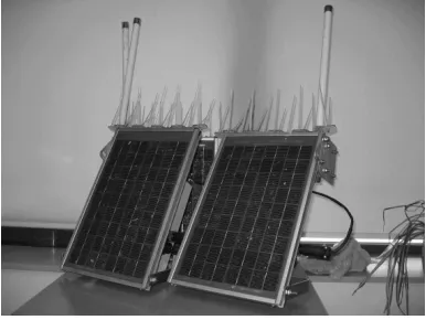
Figure 2: A FloodNET sensor node on site.

Figure 3: FloodNET sensor nodes.

several wireless sensor nodes to form a WSN system that monitors the water level in the River Crouch, East Essex in Eastern England [9]. The principle aim of FloodNET is to give at least two hours warning before flooding occurs, such that actions can be taken to alleviate risks to people and property. This early and precise prediction is crucial as there is a clear correlation between the cost of damage and both the time in advance any warnings are given and the depth of the flooding.

At present, FloodNET consists of twelve nodes, each of which (shown in figures 2 and 3) includes a BitsyX Single Board Computer and Intel’s 400MHz PXA255 RISC micro-processor. This processor is in sleep mode most of the time since it consumes a significant amount of power (1000mW) when providing field processing capabilities. The board pro-vides support for PCMCIA where a wireless LAN PC card is installed to transfer or receive data wirelessly from the neighbourhood (requires an additional 910mW and 640mW of power respectively). The node’s sensor module contains two analog-to-digital converters and a water-depth trans-ducer sensor. The converters are always turned on (requires 20mW power), while the sensor itself operates with another additional 50mW. Each node is installed with a solar panel in conjunction with a 12V 12Ah/20hr battery as a power source.

Thus, FloodNET nodes take measurements and store them locally on the memory with very little power (around 70mW) relative to that of activating the single board computer and transmitting data (around 1910mW). Moreover, nodes are

capable of communicating over a range of around 600 to 800 metres. A combination of this and the presence of obstruc-tions such as sea walls, trees, and buildings at the Flood-NET field site, means that most nodes do not have a direct link with the base-station. Therefore a node communicates with its neighbours and passes data using a wireless IEEE 802.11 Ethernet Network with the objective of transmitting the data back to the base-station.

3.2

The Simulator

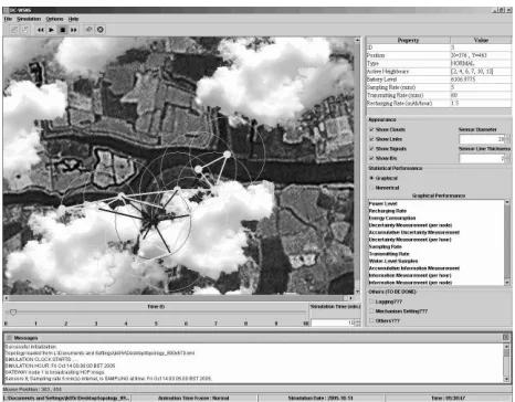
In order to evaluate our work, before we deploy it for real, we built a wireless sensor network simulator (DC-WSNS). This provides a virtual environment in which sensor nodes can ei-ther be scattered randomly or situated at specific locations. The domain models upon which DC-WSNS are built include the node, the battery, and the energy harvesting capabili-ties (specifically a solar panel model in combination with a cloud cover model). The network stack model (including the routing table and the message queue) are adapted from those in the ARA simulator [16]. At the current stage of our simulator, nodes can fail due to their battery depletion, but they can not be added or removed during the course of a simulation run.

Specifically, in our case, the nodes in the network deplete their energy resources at different rates (as the nodes have different sampling, transmitting, and receiving rates). More-over, a model of battery charging needs to be incorporated, in addition to that of a static battery model, because Flood-NET’s nodes have solar panels as one of their energy pro-ducing components. For such solar powered systems, a key issue is that of the amount of sunlight available; this is given by the time of day (i.e. there is no sunlight at night) and the cloud cover (i.e. if it is very cloudy then the panels will receive little sunlight). In modelling the clouds, we consider their shape, their thickness, their speed, and their move-ments in variable directions (see figure 4). With the cloud model, one form of energy recharging (using a solar panel) is to assume that if a solar panel does not lie under a cloud, it will gain a preset energy increase each day. However, this energy will be reduced depending on the number of layers or the thickness of the cloud above the solar panel. The thicker or the more layers the cloud has, the more of the sun’s energy is trapped inside, hence, the less energy is re-gained. However, during night time, due to the absence of sunlight, which is the main resource for the solar panel to convert its energy power, a node’s energy supply recharges at a small rate per hour due to stored energy in the solar cells. This rate is chosen arbitrarily and remains constant during the night time. Whilst during day time, the energy recharging rate is modelled as a quadratic function which peaks (i.e. recharges the most) at midday. With all these models, DC-WSNS provides a platform in which objective observations can be made at any time.

Figure 4: DC-WSNS simulation. FloodNET’s nodes (represented by the filled dots) transmit their col-lected samples back to the base-station (using multi-hop routing).

consumption. However, the nodes are programmed to ig-nore and drop packets that are not destined to them for the purpose of energy savings. Incorporating a more real-istic network communication model into our simulator will be part of our future work.

4.

PROBLEM REPRESENTATION

Before we detail our decentralised control algorithm, we first formalize the problem we are addressing in this work. Let

nbe the number of sensors in the system and the set of all sensors beI={i1, ..., in}. Each sensor i∈I hass actions it can perform and they are denoted asCi_={ci

1, ...cis}. In our adaptive sampling context, these actions represent the hourly sampling rate that a sensor can opt to perform at any particular point of time during its lifetime. For instance, by setting its sampling action toci

x, sensor ichooses to sense the environmentcixtimes per hour. Thus, a sensor can only elect one action at any particular point of time, however it can then choose a differentcixat subsequent decision points. This means a sensor is allowed to adjust its action (by de-creasing or inde-creasing its sampling rate) based on its past set of observed data and the set of data that it believes it will observe.

At this time, FloodNET’s system consists of twelve sen-sors (n = 12). For the sake of simplicity and in order to exploit all the possible changes in the system, there are four different actions (s = 4) describing the sensor’s sampling rate. A sensor can either sample one, three, six, or twelve times in every hour (i.e.Ci={1,3,6,12},∀i). Moreover, as FloodNET’s raw-data shows a similar pattern between days, with two tides coming in and out (with±one hour delay), we set the sampling schedules of each sensor based upon its previous day’s data values. For this purpose, we have a fixed window size ofh= 1..24 (such that each element rep-resents a one hour slot, for instance 1 reprep-resents the slot be-tween 00:00am and 01.00am). Each sensor, thus, has its own hourly-based schedule per day, denoted asAi_={ai

1, ..., ai24} where ai

h ∈ Ci. Additionally, there is a resource cost as-sociated with sampling data. This resource is provided by

the limited battery power installed on each sensor and the solar energy panel that is capable of recharging the battery state. Assuming that the remaining battery power left for sensor iat the beginning of a day is E_{r, and it requires a}i certain amount of energy es to sample an event, then the sum of all the energy required to do the sampling actions on that day must not exceed the remaining battery power (i.e. P24

x=1a i

xes≤Eri).

Each FloodNET node is capable of measuring its battery voltage at any particular point of time. However, under real life conditions, voltage measurements alone can be very mis-leading to estimate the remaining battery capacity. This is due to the chemical reactions within the cells such that the capacity of a battery is dependent on the discharge condi-tions including the magnitude of the current, the duration of the current, the allowable terminal voltage of the bat-tery, the temperature, the condition (whether it is new or old), and the historical usage (whether it has been over-discharged). At this point, our simulator just assumes that the deployed agents have access to the true value of the remaining energy left in the batteries. More realistic calcu-lation in which the recalcu-lationship between current, discharge time, and capacity for a lead acid battery is expressed by Peukert’s law [11] will be considered as a future work for real deployment purposes.

4.1

The Information Metric

To operate effectively, our system needs a means of valuing the various observations that the sensors may make. Specif-ically, we use a valuation function which defines the value of an outcome for an action. In short, it is this function that the system is trying to maximise and which describes the properties that we would like the overall system’s outcomes to possess. Now, there are many methods by which the value of information can be determined, including simple linear regression [10] and the Kalman Filter [5, 12]. However, we chose the former, which is based on the uncertainty values of the regression line, as most of the time the relationship between the time and water-level raw-data can be graphed as a straight line. In FloodNET’s data model, by sampling more, a sensor will necessarily get a lower uncertainty er-ror. Now, this uncertainty is expressed in confidence bands about the linear regression line that we perform with our water-level raw-data. In fact, the uncertainty error has the same interpretation as the standard deviation of the residu-als (termedsein equation 2, whereprepresents the number of data points, ˆyis the new value of y calculated from the newly found slope and intercept variables), except that it varies according to the location along the regression line. The distance of the confidence bands from the regression line (σ) is:

σ=se s

1

p+

(x∗_−x¯)2 P

(xi−x¯)2

(1)

where se is the standard error of the estimate, x∗ is the location along the x-axis data points where the distance is being calculated, and ¯xis the mean value of X.

se= s

P₍

yi−ˆyi)2

p−2 (2)

because if there are only two data points they will produce a smooth linear regression line (with no uncertainty error), while anything less than that will result in invalid inputs. For these reasons, we assume that a sensor must at least sample once in an hour slot (defined as the minimum sam-pling rate, thereforeEi

r ≥24es, where i∈I). In this way, given the uncertainty error, we are able to tell whether one set of observations is more valuable than another, therefore, it can help us to define a value associated to every action. Here, we derive the values as the reduction in uncertainty error that a sensor can achieve by taking more samples than the minimum sampling rate. This minimum sampling rate is applied as a basis where a sensor gains zero value/profit. The data values for each sensor are often best represented in a table format, as shown in table 1 (values are arbitrary, for illustrative purpose). In this table, the columns represent the hour slot, for instance wherecolumn= 3, if this partic-ular sensor chooses to sense three, six, or twelve times, in return it will gain a corresponding reduction in uncertainty error of 27.59, 43.79 and 55.23 compared to if it had only taken one sample during the same period.

As described later in section 5, during the first day of a simulation, every sensor is designed to sample at its maxi-mum rate. Now, by taking subsets of samples (correspond-ing to the set of actions specified in the table’s row header) from the full set and performing the linear regression on these subsets, we obtain a new value of uncertainty error for each subset. The values that will be assigned to the ta-ble are the uncertainty error difference between sampling at the minimum rate and at other rates. For instance where

column= 3, if the uncertainty error that is produced with a subset of samples c2 with three samples taken between 02:00am and 03.00am has a value of 128.66, while that of a minimum sampling rate c1 with only one sample taken between the same period is 156.25, then the value inside

column= 3 androw= 2, will be 27.59.

5.

THE DECENTRALISED ALGORITHM

Having described our representation, we now focus on how to search for sets of sensor’s schedules that maximise the data values, which in turn, will reduce the total uncertainty error of information collected at the base-station. For these purposes, we introduce V as as×t matrix withs number of actions andtnumber of hours:

Vi₌

2

6 4

vi

11 v12i . . . v1it ..

. ... . .. ...

vis1 vis2 . . . vsti 3

7 5 D

i₌

2

6 4

di

11 di12 . . . di1t ..

. ... . .. ...

dis1 dis2 . . . dist 3

7 5

vi

xy now represents the value that a sensoriwill get if it chooses to perform actionci

x in hour slot y. D is a matrix of binary values and each of the elements corresponds to a decision variable (a “1” and a “0” respectively represent the agreement and the refusal to carry out the correspondingci

x action). For instance, whendi

11= 1 then the sensor agrees to perform actionci1 in hour slot 1. This also means that

di

x1= 0,∀x∈Ci\ci1.

Given that, at the beginning of each day, a sensor knows the maximum number of samplesNs (Ns≥24) it can take on that particular day, a sensor is designed to select those actions that reduce the uncertainty the most (i.e. maximise the value gained, as defined in equation 3) subject to some

1 2 3 ... 24

1 Sample (c1) 0 0 0 ... 0

3 Samples (c2) 0.29 1.21 27.59 ... 3.88

6 Samples (c3) 0.31 1.51 43.79 ... 8.92

12 Samples (c4) 0.33 1.55 55.23 ... 13.45

Table 1: Action-Value Table.

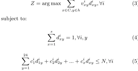
system constraints. Specifically, the constraint in equation 4 states that a sensor can only elect one action at any particu-lar point of time, whereas that in equation 5 states that the total number of samples taken by a sensor must not exceed the maximum number of samples it can take on that day:

Z = arg max X x∈C,y∈h

vxyi d i

xy,∀i (3)

subject to:

s X

x=1

dixy= 1,∀i, y (4)

24 X

y=1

ci1d i 1y+c

i 2d

i

2y+...+c i xd

i

xy≤N,∀i (5)

The problem we face in this adaptive sampling context is a linear programming problem, in general, and the person-task assignment problem in particular [15]. In the assign-ment problem, the aim is to assign a set of people to do a set of tasks. Each person takes a certain number of minutes to do a certain task, or cannot do a particular task at all, and each person can be assigned to exactly one task. The aim is to minimize the total time taken to do all of the tasks. In general, where there are n persons and tasks, there are n! possible assignments. This may seem a small space to search for, but for instance if there are 20 persons for 20 tasks in a medium-sized company, then there are 1026

possible assign-ments (which is intractable in a reasonable amount of time). Our problem can, thus, be cast as the person-task assign-ment problem as they are strongly similar in nature. Given this insight, our problem can be solved using binary integer programming (BIP) [1], which is a subset of linear program-ming, with a search space of 324

possible assignments. Now, a popular method to solve our problem numerically is the simplex algorithm, and in this case we exploit the GNU Lin-ear Programing Kit (GLPK)1

.

Having described the technique that we use, we now seek to present the rest of our decentralised algorithm (see algo-rithm 1). Specifically, the algoalgo-rithm, which is distributed and installed on each sensor in the network, provides a means for the individual nodes to make local decisions (to alter its own sampling rate based upon its observations, both on its past sets and on the future sets it believes it will ob-serve). Now, at the beginning of a simulation, some required variables are initialized. These include theupdSSched boo-lean variable which is given the valueT RU E. It represents the mode that a sensor is currently in at any particular point of time. In our simulation, there are two possibilities; (i) normal mode and (ii) sampling schedule updating mode. In the former case, a sensor sets its hourly sampling rate based upon its current schedule that it has already computed and

1

Algorithm 1Schedule-Based Adaptive Sampling. 1: updSSched←T RU E

2: sRate←M AX S RAT E

3: readings← {}

4: loop

5: if sTime =N OW _then

6: readings←PerformSampling(N OW)

7: if¬updSSchedthen 8: hour←Hour(N OW)

9: sRate←GetSRate₍hour₎

10: end if

11: SetSTime_{(sTime + sRate)} 12: end if

13: if tTime =N OW then

14: uError←CalcUError_(readings) 15: ifdateChanged then

16: daysCount←daysCount + 1

17: if updSSchedthen

18: CalcUReduction_(uError)

19: FindSSchedule(uError) .BIP

20: updSSched←F ALSE

21: end if 22: end if

23: if ¬updSSched ∧ HasEnoughEnergy() ∧

(daysCount≥CON ST)then

24: updSSched←T RU E ._{Schedule updated}

25: daysCount←0

26: sRate←M AX S RAT E

27: end if 28: readings← {}

29: end if 30: end loop

stored in its memory. In the latter case, the sensor will up-date its schedule because the current one is out-of-up-date. On the first day of a simulation, all sensors are assigned to act in this mode, hence, each sensor’s sampling rate variable,

sRate, is initialized to its maximum (i.e. M AX S RAT E

in line 2). This is done such that the maximum number of samples can be utilized to evaluate the data values (which corresponds to the maximum reduction in uncertainty er-ror) a sensor will gain compared to if it had only taken fewer samples than the maximum sampling rate. On the other hand, the readings vector variable, that records all the taken samples, is initialized to the null set.

After the initialization phase, sensors follow an infinite loop state. On each iteration, each sensor checks its sam-pling and transmitting time. Whenever the current loop represents the time that a sensor needs to sample (line 5), theP erf ormReading function instantiates a new reading

and attaches it to the end of thereadingsvariable. Subse-quently, if the sensor is not in updating mode, itssRateis assigned a value equal to the sampling rate in its schedule, corresponding to the appropriate hour (line 9). The sensor then sets its nextsT imesampling time variable. Inside the same loop iteration, whenever the sensor is also required to transmit its current readings (line 13), it firstly calculates the uncertainty error in this set of readings by using the sim-ple linear regression method described in section 4.1. Later, if the sensor detects that it has entered the following day, it will call the CalcU Reduction function to compute the reduction in uncertainty error that the sensor can achieve by taking more samples than the minimum sampling rate. For this purpose, we use the BIP GLPK solver to evaluate the optimal sets of sensor schedules that maximise the un-certainty error reduction, given the sensors’ current energy constraints (line 19).

Now, due to the fact that we partition the simulation time into hour slots, and while the FloodNET tides in and out actually differ in a range of half an hour to an hour between days, there is a necessity to update the sensors’ schedules pe-riodically. Otherwise, the schedule will be out of sync and the algorithm will perform poorly. In the schedule updating mode, a sensor is again required to perform sampling at its maximum rate (line 26). Therefore, theHasEnoughEnergy

procedure basically checks the sufficiency of the sensor’s re-maining battery to perform this task. And whenever all the other requirements have been met (line 23), the sensor en-ters this mode once again. At the end of the transmitting phase, thereadingsvariable is cleared.

6.

EMPIRICAL EVALUATION

Having described our algorithm, we now seek to evaluate its effectiveness by comparing it against a standard non-adaptive approach in which each sensor in the network di-vides the total number of samples it can perform in a day equally into its hour slots. Specifically, we are interested in comparing the cumulative uncertainty error of informa-tion gathered at the base-stainforma-tion and the uncertainty error of information collected hourly. We chose these two mea-sures because they enable us to determine whether by using the same amount of battery energy, our adaptive sampling algorithm permits the sensors to collect more valuable infor-mation that has lower uncertainty error compared to that of the non-adaptive one.

In our experiments, we use the actual FloodNET data for batteries, tides readings, and cloud cover. We do this because we want to mimic the FloodNET scenario as re-alistically as possible. All the cloud parameters (including the cloud coverage, wind speed, and cloud thickness) are initialized with realistic data (at FloodNET’s site) available in Meteorological Aviation Routine Report (METAR) for-mat2

. The experiments are also run using FloodNET’s ac-tual topology with a fixed number of nodes (twelve) at fixed locations (i.e. the nodes are immobile). The remaining bat-tery energy of each sensor and its recharging rate are set to be so low that it is not capable of sampling at its maximum rate. Now, given these constraints, sensors must therefore schedule themselves to determine how often and when to sample efficiently in order to minimise their uncertainty er-ror.

The sampled data model (worth approximately nine days of measured data starting from Oct 14th _{2006 00.00AM)} for each node was fixed for each instance of the experi-ment. The purpose of this is to get fair comparative results and estimations. As can be seen in figure 5, our algorithm performs well; compared to the benchmark, our algorithm consistently reduces the information uncertainty by about 44.5% per day over the trial period. The plot shows the su-periority of our adaptive sampling algorithm over the non-adaptive one. The overall graphs of both algorithms are lin-ear, however as expected, the gradient of the non-adaptive algorithm is steeper than that of ours.

Additionally, figures 6 and 7 shows more clearly how our adaptive sampling algorithm achieves this performance. Af-ter leaving the schedule updating mode (i.e. the second day of a simulation, as can be seen in figure 7), a sensor is able to perform adaptive sampling by conserving its battery en-ergy in order to take more samples during the most dynamic

2

Oct 14 Oct 15 Oct 16 Oct 17 Oct 18 Oct 19 Oct 20 Oct 21 Oct 22 Oct 23 0

0.5 1 1.5 2 2.5

3x 10

5 Cumulative Uncertainty Measurement

Time (Dates are in 2006)

Uncertainty Error

Uniform Non−Adaptive Sampling

Decentralised Schedule−Based Adaptive Sampling

Figure 5: Cumulative uncertainty error of informa-tion gathered over a 9-day period plotted against time.

Oct 14 Oct 15 Oct 16 Oct 17 Oct 18 Oct 19 Oct 20 Oct 21 Oct 22 Oct 23 0

1000 2000 3000 4000 5000 6000 7000 8000

Uncertainty Measurement (per hour)

Time (Dates are in 2006)

Uncertainty Error

Uniform Non−Adaptive Sampling

Decentralised Schedule−Based Adaptive Sampling

Figure 6: Uncertainty error of information gathered hourly over a 9-day period plotted against time.

events while taking fewer samples during the static ones. In our case, the dynamic events of a tide occur at the time it comes in (specifically when the sensor rises off mud, between 07.00 and 09.00 in figure 7), reaches the peak (between 10.00 and 11.00), and goes out (between 12.00 and 14.00). During these events, sensors normally set their sampling rates to a maximum value (i.e. in our case, at five minute intervals). As a result, from the second day onward, figure 6 shows a re-duction in uncertainty error of information collected (partic-ularly during the dynamic events), except when the sensors are in updating mode (on Oct 17th_{and 20}th_).

Other benchmarks including the optimal adaptive sam-pling that is given the knowledge about all the sample read-ings and the greedy sampling in which each sensor samples at its maximum rate whenever there is enough battery en-ergy to do so, will be considered as future work.

Figure 7: Water samples gathered on the second day of the simulation. Graph only displays some selected nodes for better visibility.

7.

CONCLUSIONS

In this paper, we have focussed primarily on issues associ-ated with energy management in WSNs. In particular, we concentrated on the decentralised control of sampling strate-gies in the FloodNET system. To this end, we tackled the problem by developing a novel decentralised schedule-based adaptive sampling algorithm. The empirical results are ob-tained from the simulation run using DC-WSNS and these show that the algorithm is effective in balancing the trade-offs associated with wanting to gain as much information as possible by sampling as often as possible, with the con-straints imposed on these activities by the limited power available for these actions.

Now, although the effectiveness of this work is evaluated in terms of the FloodNET domain, the challenges that are involved here are very similar to those that occur in the design of many other WSNs. Specifically, many WSNs are being deployed in the domain of environmental phenomena monitoring (e.g. soil moisture and habitat monitoring) that typically show a periodic pattern in their readings (as we have with the tides). Thus, the algorithm can be used and transferred simply by altering the time period over which the readings are spread. The simple linear regression tool for evaluating the value of information can also be applied to those WSNs in which the relationship between the time and reading (with associated noise and uncertainty) is lin-ear or piecewise-linlin-ear. The linlin-ear programming technique, together with the utility function and constraints, can be adapted to meet the design objectives of other WSNs in general. While the simulator can be utilized to simulate different kinds of WSN scenarios (with the battery and so-lar panel as the sensors’ energy-producing components) by modifying the configuration topology file.

FloodNET sensors to deliver readings as soon as possible (whenever necessary) in the case of flooding. In the later, we need to deploy our algorithm on the actual sensors and ensure the data it needs to operate is provided in a timely manner.

8.

REFERENCES

[1] C. S. Chen, M. S. Kang, J. C. Hwang, and C. W. Huang. Application of binary integer programming for load transfer ofdistribution systems. InPowerCon 2000 - International Conference on Power System Technology. Proceedings (Cat. No.00EX409), pt. 1, volume 1, pages 305–10, 2000.

[2] K. Chintalapudi, T. Fu, J. Paek, N. Kothari, S. Rangwala, J. Caffrey, R. Govindan, E. Johnson, and S. Masri. Monitoring civil structures with a wireless sensor network.IEEE Internet Computing, 10(2):26–34, March/April 2006.

[3] R. K. Dash, N. R. Jennings, and D. C. Parkes. Computational mechanism design: A call to arms.

IEEE Intelligent Systems, 18(6):40–7, November/December 2003.

[4] D. deRoure. Floodnet: A new flood warning system.

Ingenia, 23:49–51, 2005.

[5] C. Guestrin, A. Krause, and A. P. Singh. Near optimal sensor placements in gaussian processes. In

ICML 2005 - Proceedings of the 22nd International Conference on Machine Learning, pages 265–272, 2005.

[6] N. R. Jennings. An agent-based approach for building complex software systems.Communications of the ACM, 44(4):35–41, April 2001.

[7] G. Mainland, D. C. Parkes, and M. Welsh.

Decentralized, adaptive resource allocation for sensor networks. InProceedings of the 2nd USENIX/ACM Symposium on Networked Systems Design and Implementation (NSDI 2005), pages 315–28, 2005. [8] K. Martinez, J. K. Hart, and R. Ong. Glacial

environment monitoring using sensor networks. In

Proceedings of Real-World Wireless Sensor Networks, Stockholm, Sweden, 2005.

[9] J. Neal, P. Atkinson, and C. Hutton. Floodnet: An enkf based forecasting system for the assimilation of spatial data from an adaptive monitoring network into a flood inundation model. evaluation in a tidal estuary. Technical report, GeoData Institute, University of Southampton, UK, 2006. [10] P. Padhy, R. K. Dash, K. Martinez, and N. R.

Jennings. A utility-based sensing and communication model for a glacial sensor network. InProc. 5th Int. Conf. on Autonomous Agents and Multi-Agent Systems, pages 1353–1360, Hakodate, Japan, 2006. [11] V. Pop, H. J. Bergveld, P. H. L. Notten, and P. P. L.

Regtien. State-of-the-art of battery state-of-charge determination.Measurement Science and Technology, 16(12):R93–R110, December 2005.

[12] A. Rogers, R. K. Dash, N. R. Jennings, S. Reece, and S. Roberts. Computational mechanism design for information fusion within sensor networks. In

Proceedings of The 9th International Conference on Information Fusion, Florence, Italy, 2006.

[13] G. Simon, G. Balogh, G. Pap, M. Maroti, B. Kusy, J. Sallai, A. Ledeczi, A. Nadas, and K. Frampton.

Sensor network-based countersniper system. In

SenSys’04 - Proceedings of the Second International Conference on Embedded Networked Sensor Systems, pages 1–12, 2004.

[14] R. Willett, A. Martin, and R. Nowak. Backcasting: adaptive sampling for sensor networks. InProceedings of the 3rd International Symposium on Information Processing in Sensor Networks (IEEE Cat.

No.04EX890), pages 124–33, 2004.

[15] B. C. Yong, T. Kurokawa, Y. Takefuji, and S. K. Hwa. An o(1) approximate parallel algorithm for the n-task-n-person assignment problem. InIJCNN ’93-Nagoya. Proceedings of 1993 International Joint Conference on Neural Networks (Cat.

No.93CH3353-0), pt. 2, volume 2, pages 1503–6, 1993. [16] J. Zhou, D. deRoure, and S. Vivekanandan. Adaptive