S. Chen1, X. Hong2, and C.J. Harris1 1
School of Electronics and Computer Sciences, University of Southampton, Southampton SO17 1BJ, U.K.
{sqc,cjh}@ecs.soton.ac.uk
2 School of Systems Engineering, University of Reading, Reading RG6 6AY, U.K.
Abstract. A unified approach is proposed for sparse kernel data mod-elling that includes regression and classification as well as probability density function estimation. The orthogonal-least-squares forward selec-tion method based on the leave-one-out test criteria is presented within this unified data-modelling framework to construct sparse kernel models that generalise well. Examples from regression, classification and den-sity estimation applications are used to illustrate the effectiveness of this generic sparse kernel data modelling approach.
1
Introduction
The objective of modelling from data is not that the model simply fits the training data well. Rather, the goodness of a model is characterised by its gener-alisation capability, interpretability and ease for knowledge extraction. All these desired properties depend crucially on the ability to construct appropriate sparse models by the modelling process, and a basic principle in practical data modelling is the parsimonious principle of ensuring the smallest possible model that ex-plains the training data. Recently considerable research efforts have been focused on sparse kernel data modelling techniques [1,2,3,4,5,6]. Sparse kernel modelling methods typically use every training input data as a kernel. A sparse representa-tion is then sought based on various criteria by making as many kernel weights to (near) zero values as possible. A different approach to these sparse kernel modelling methods is the forward selection using the orthogonal least squares (OLS) algorithm [7,8], developed in the late 80s for nonlinear system modelling, which remains highly popular for data modelling practicians.
Since its derivation, many enhanced variants of the OLS forward-selection algorithm have been proposed by incorporating the new developments from ma-chining learning and the approach has extended its application to all the areas of data modelling, including regression, classification and kernel density estimation [9,10,11,12,13,14,15]. This contribution continues this theme, and it presents a unified framework for sparse kernel modelling that include all the three classes of data modelling applications, namely, regression, classification and probability density function (PDF) estimation. Based on this unified data-modelling frame-work, the OLS forward selection algorithm using the leave-one-out (LOO) test
H. Yin et al. (Eds.): IDEAL 2007, LNCS 4881, pp. 27–36, 2007. c
criteria and local regularisation (LR) is employed to construct sparse kernel mod-els with excellent generalisation capability. Experimental results are included to demonstrate the effectiveness of the OLS forward selection algorithm based on the LOO test criteria within the proposed unified data-modelling framework.
2
A Unified Framework for Data Modelling
Given the training data set, DN = {xk, yk}Nk=1, where xk =
[x1,k x2,k· · ·xm,k]T ∈ Rm is an observation sample and yk is the target or
desired response forxk, the task is to infer a kernel model of the form
ˆ
y= ˆf(x;βN, ρ) =
N
i=1
βiKρ(x,xi) (1)
to capture the underlying data generating mechanism, where ˆydenotes the model output, βN = [β1 β2· · ·βN]T is the kernel weight vector and Kρ(•,•) is the
chosen kernel function with a kernel widthρ. Many types of kernel function can be employed and a commonly used one is the Gaussian function of the form
Kρ(x,ck) =
1 (2πρ2)m/2e
−x−ck2
2ρ2 , (2)
where ck ∈ Rm is the k-th kernel centre vector. For regression and
classifica-tion problems, the factor 1
(2πρ2)m/2 can be combined into kernel weightsβi. The generic kernel model (1) is defined by placing a kernel at each of the training input samplesxk and forming a linear combination of all the bases defined on
the training data set. A sparse representation is then sought by selecting only Nssignificant regressors from the full regressor set, whereNsN.
The underlying data generating mechanism is governed byy=f(x)+ε, where εis a white process representing the observation noise. For regression problems, the unknown mappingf :Rm→ R. Regression is a supervised learning problem, as the desired responseyk ∈ Rfor the training data point xk is given. For
two-class two-classification problems, the unknown mappingf : Rm → {−1,+1}. The estimated class label for the pattern vectorxk is given by ˜yk = sgn(ˆyk) with
sgn(y) =
−1, y≤0,
+1, y >0. (3) Classification is also a supervised learning problem, since the correct label yk ∈ {−1,+1} for the training data point xk is provided. For PDF estimation
problems, the data{xk}Nk=1 are drawn from a unknown density f :R
m→ R
+.
Becausef is a PDF,f(x)≥0 forx∈ RmandRmf(u)du= 1. Thus, a kernel in
a kernel density estimate must satisfyKρ(x,ck)≥0 and
RmKρ(u,ck)du= 1.
Moreover the kernel weights must satisfy the nonnegative constraint
and the unity constraint
βTN1N = 1, (5)
where1Ndenotes the vector of ones with dimensionN. Kernel density estimation
is an unsupervised learning problem because the desired response is unknown for each training data pointxk. This difficult is circumvented by “inventing” a
target functionyk forxk, so that the problem becomes a constrained regression
one with the constraints (4) and (5). In particular, we chooseyk to be the value
of the Parzen window estimate [16,17] at point xk. This choice of the desired
response for density estimation is fully justified in [13].
Let the modelling error at training data pointxk be k=yk−yˆk, where
ˆ
yk = [Kρ(xk,x1)Kρ(xk,x2)· · ·Kρ(xk,xN)]βN =φ T
(k)βN. (6)
Define Φ = [φ1 φ2· · ·φN] with φk = [Kρ(x1,xk)Kρ(x2,xk)· · ·Kρ(xN,xk)] T
for 1≤k≤N,y= [y1 y2· · ·yN]T and= [12· · ·N]T. The regression model
(1) over the training data setDN can then be expressed in the matrix form
y=Φ βN +. (7)
Let an orthogonal decomposition of the regression matrix Φ be Φ = W AN,
whereAN is theN×N upper triangular matrix with unity diagonal elements,
andW= [w1w2· · ·wN] with orthogonal columns satisfyingwTi wj = 0, ifi=j.
The regression model (7) can alternatively be expressed as
y=W gN +, (8)
where the weight vector gN = [g1 g2· · ·gN]T satisfies the triangular system
ANβN =gN. The model (6) is equivalently expressed by
ˆ
yk =wT(k)gN, (9)
wherewT(k) = [w
k,1 wk,2· · ·wk,N] is thek-th row ofW.
3
Orthogonal-Least-Squares Algorithm
As established in the previous section, the regression, classification and PDF estimation can all be unified within the common regression modelling framework. Therefore, the OLS forward selection based on the LOO test criteria and local regularisation (OLS-LOO-LR) [10] provides an efficient algorithm to construct a sparse kernel model that generalise well.
3.1 Sparse Kernel Regression Model Construction
The LR aided least squares solution for the weight parameter vectorgN can be
obtained by minimising the following regularised error criterion [11]
whereλ = [λ1 λ2· · ·λN]T is the vector of regularisation parameters, andΛ =
diag{λ1, λ2,· · ·, λN}. Applying the evidence procedure results in the following
iterative updating formulas for the regularisation parameters [9]
λnewi = γ
old
i
N−γold
T g2
i
, 1≤i≤N, (11)
wheregi for 1≤i≤N denote the current estimated parameter values, and
γ=
N
i=1
γi with γi=
wTi wi
λi+wTi wi
. (12)
Typically a few iterations (less than 10) are sufficient to find a (near) optimalλ. The use of LR is known to be capable of providing very sparse solutions [2,11]. For regression, the OLS-LOO-LR algorithm selects a sparse model by incre-mentally minimising the LOO mean square error (MSE) criterion, which is a measure of the model’s generalisation performance [10,14,18]. At then-th stage of the OLS selection procedure, ann-term model is selected. The LOO test error, denoted as(kn,−k), for the selected n-term model is defined as [10,14]
k(n,−k)=k(n)/ηk(n), (13)
where(kn) is the usualn-term modelling error and ηk(n) is the associated LOO error weighting. The LOO MSE for the model with a sizenis then defined by
Jn=
1 N
N
k=1
(kn,−k)
2
= 1 N
N
k=1
(kn)
2
/
η(kn) 2
. (14)
This LOO MSE can be computed efficiently due to the fact that(kn) and ηk(n) can be calculated recursively according to [10,14]
k(n)=k(n−1)−wk,ngn (15)
and
ηk(n)=η(kn−1)−w2k,n/wTnwn+λn
, (16)
respectively, wherewk,n is thek-th element ofwn. The selection is carried out
as follows. At then-th stage of the selection procedure, a model term is selected among the remainingntoN candidates if the resultingn-term model produces the smallest LOO MSEJn. The selection procedure is terminated when
JNs+1≥JNs, (17)
yielding anNs-term sparse model. The LOO statisticJnis at least locally convex
with respect to the model sizen[14]. Thus, there exists an “optimal” model size Ns such that for n ≤Ns Jn decreases as n increases while the condition (17)
Initialisation: Set λi= 10−6for 1≤i≤N, and set iteration indexI= 1. Step 1: Given the currentλand with the following initial conditions
(0)k =yk, η
(0)
k = 1, 1≤k≤N, andJ0=yTy/N, (18)
use the OLS-LOO procedure [10] to select a subset model withNI terms. Step 2: Updateλusing (11) and (12) with N=NI. If the maximum iteration
number (e.g. 10) is reached, stop; otherwise setI+ = 1 and go toStep 1.
3.2 Sparse Kernel Classifier Construction
The same LOO cross validation concept [18] is adopted to provide a measure of classifier’s generalisation capability. Denote the test output of the LOOn-term model evaluated at thek-th data sample ofDN not used in training as ˆy
(n,−k)
k .
The associated LOO signed decision variable is defined by s(kn,−k)= sgn(yk)ˆy
(n,−k)
k =ykyˆ
(n,−k)
k , (19)
where sgn(yk) =yk since the class labelyk ∈ {−1,+1}. The LOO
misclassifica-tion rate can be computed by
Jn=
1 N
N
k=1
Id
s(kn,−k)
, (20)
where the indication function is defined byId(y) = 1 ify ≤0 andId(y) = 0 if
y >0. The LOO misclassification rate Jn can be evaluated efficiently because
s(kn,−k) can be calculated very fast [15]. Specifically, express the LOO signed decision variable ass(kn,−k)=ψk(n)/η(kn). The recursive formula forη(kn) is given in (16), whileψk(n)can be represented using the recursive formula [15]
ψk(n)=ψ(kn−1)+ykgnwk,n−w2k,n/
wTnwn+λn
. (21) The OLS-LOO-LR algorithm described in Subsection 3.1 can readily be ap-plied to select a sparse kernel classifier with some minor modifications. Moreover, extensive empirical experience has suggested that all the regularisation param-etersλi, 1≤i≤N, can be set to a small positive constant λ, and there is no
need to update them using the evidence procedure. The sparse kernel classifier selection procedure based on this OLS-LOO algorithm is now summarised.
Settingλto a small positive number, and with the following initial conditions ψ(0)k = 0 and ηk(0)= 1 for 1≤k≤N, and J0= 1, (22)
use the OLS-LOO procedure [15] to select a subset model withNsterms.
The LOO misclassification rateJn is also locally convex with respect to the
classifier’s size n. Thus there exists an optimal model size Ns such that for
n≤NsJn decreases as nincreases, whileJNs ≤JNs+1. Therefore the selection
3.3 Sparse Kernel Density Estimator Construction
Since the kernel density estimation problem can be expressed as a constrained regression modelling, the OLS-LOO-LR algorithm detailed in Subsection 3.1 can be used to select a sparse kernel density estimate. After the structure de-termination using the OLS-LOO-LR algorithm, a sparseNs-term subset kernel
model is obtained. LetANs denote the subset matrix of AN, corresponding to
the selected Ns-term subset model. The kernel weight vector βNs, computed
fromANsβNs =gNs, may not satisfy the constraints (4) and (5). However, we
can recalculateβNsusing the multiplicative nonnegative quadratic programming (MNQP) algorithm [3,6]. SinceNsis very small, the extra computation involved
is small. Formally, this task is defined as follows. FindβNs for the model
y=ΦNsβNs+, (23)
subject to the constraints
βi≥0, 1≤i≤Ns, (24)
βTN
s1Ns= 1, (25)
where ΦNs denotes the selected subset regression matrix and β T
Ns =
[β1β2· · ·βNs]. The kernel weight vector can be obtained by solving the following
constrained nonnegative quadratic programming min
βNs{
1 2β
T
NsCNsβNs−v T NsβNs}
s.t.βTN
s1Ns = 1 andβi≥0, 1≤i≤Ns,
(26)
where CNs = Φ T
NsΦNs = [ci,j] ∈ R
Ns×Ns is the related design matrix and
vNs = Φ
T
Nsy = [v1 v2· · ·vNs]
T. Although there exists no closed-form solution
for this optimisation problem, the solution can readily be obtained iteratively using a modified version of the MNQP algorithm [3].
Specifically, the iterative updating equations forβNs are given by [6,13]
ri<t>=βi<t> ⎛ ⎝Ns
j=1
ci,jβj<t>
⎞ ⎠
−1
, 1≤i≤Ns, (27)
h<t>= N
s
i=1
r<t>i −1
1−
Ns
i=1
ri<t>vi
, (28)
βi<t+1>=r<t>i vi+h<t>
, (29)
where the superindex<t> denotes the iteration index andhis the Lagrangian
Table 1. Comparison of modelling accuracy for the Boston housing data set. The results were averaged over 100 realizations and quoted as the mean±standard deviation.
algorithm model size training MSE test MSE OLS-LOO-LR58.6±11.3 12.9690±2.6628 17.4157±4.6670
SVM 243.2±5.3 6.7986±0.4444 23.1750±9.0459
4
Empirical Data Modelling Results
Boston Housing Data Set. This was a regression benchmark data set, avail-able at the UCI repository [19]. The data set comprised 506 data points with 14 variables. The task was to predict the median house value from the remain-ing 13 attributes. From the data set, 456 data points were randomly selected for training and the remaining 50 data points were used to form the test set. Because a Gaussian kernel was placed at each training data sample, there were N= 456 candidate regressors in the full regression model (1). The kernel width for the OLS-LOO-LR algorithm was determined via a grid-search based cross validation. The support vector machine (SVM) algorithm with theε-insensitive cost function was also used to construct the regression model for this data set, as a comparsion. The three learning parameters of the SVM algorithm, the ker-nel width, error-band and trade-off parameters, were tuned via cross validation. Average results were given over 100 repetitions, and the two sparse Gaussian kernel models obtained by the OLS-LOO-LR and SVM algorithms, respectively, are compared in Table 1.
For the particular computational platform used in the experiment, the recorded average run time for the OLS-LOO-LR algorithm when the kernel width was fixed was 200 times faster than the SVM algorithm when the kernel width, error-band and trade-off parameters were chosen. It can be seen from Table 1 that the OLS-LOO-LR algorithm achieved better modelling accuracy with a much sparser model than the SVM algorithm. The test MSE of the SVM algorithm was poor. This was probably because the three learning paremeters, namely the kernel width, error-band and trade-off parameters, were not tuned to the optimal values. For this regression problem of input dimension 13 and data sizeN ≈500, the grid search required by the SVM algorithm to tune the three learning parameters was expensive and the optimal values of the three learning parameters were hard to find.
Table 2.Average classification test error rate in % over the 100 realizations of the diabetes data set. The first 7 results were quoted from [20].
algorithm test error rate model size RBF-Network 24.29±1.88 15 AdaBoost RBF-Network 26.47±2.29 15 LP-Reg-AdaBoost 24.11±1.90 15 QP-Reg-AdaBoost 25.39±2.20 15 AdaBoost-Reg 23.79±1.80 15
SVM 23.53±1.73 not available Kernel Fisher Discriminant 23.21±1.63 468
OLS-LOO 23.00±1.70 6.0±1.0
no average model size was given in [20] but it could safely be assumed that it was much larger than 40. The kernel Fisher discriminant was the non-sparse optimal classifier using all theN = 468 training data samples as kernels.
The OLS-LOO algorithm was applied to construct sparse Gaussian kernel classifiers for this data set, and the results averaged over the 100 realisations are also listed in Table 2. It can be seen that the proposed OLS-LOO method compared favourably with the existing benchmark RBF and kernel classifier construction algorithms, both in terms of classification accuracy and model size.
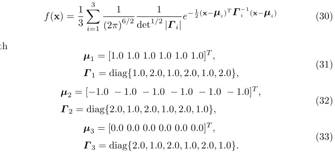
Six-dimensional density estimation. The underlying density to be estimated was given by
f(x) = 1 3
3
i=1
1 (2π)6/2
1 det1/2|Γi|
e−12(x−μi) TΓ−1
i (x−μi) (30)
with
μ1= [1.0 1.0 1.0 1.0 1.0 1.0]T,
Γ1= diag{1.0,2.0,1.0,2.0,1.0,2.0},
(31)
μ2= [−1.0 −1.0 −1.0 −1.0 −1.0 −1.0]T,
Γ2= diag{2.0,1.0,2.0,1.0,2.0,1.0},
(32)
μ3= [0.0 0.0 0.0 0.0 0.0 0.0]T,
Γ3= diag{2.0,1.0,2.0,1.0,2.0,1.0}.
(33)
A training data set ofN = 600 randomly drawn samples was used to construct kernel density estimates, and a separate test data set ofNtest= 10,000 samples
was used to calculate theL1test error for the resulting estimate according to
L1=
1 Ntest
Ntest
k=1
f(xk)−fˆ(xk;βN, ρ). (34)
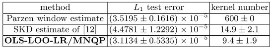
Table 3.Performance comparison for the six-dimensional three-Gaussian mixture
method L1 test error kernel number Parzen window estimate (3.5195±0.1616)×10−5 600±0
SKD estimate of [12] (4.4781±1.2292)×10−5 14.9±2.1 OLS-LOO-LR/MNQP(3.1134±0.5335)×10−5 9.4±1.9
Simulation was used to test the proposed combined OLS-LOO-LR and MNQP algorithm and to compare its performance with the Parzen window estimator as well as our previous sparse kernel density (SKD) estimation algorithm [12]. The algorithm of [12], although also based on the OLS-LOO-LR regression frame-work, is very different from the current combined OLS-LOO-LR and MNQP algorithm. In particular, it transfers the kernels into the corresponding cumula-tive distribution functions and uses the empirical distribution function calculated on the training data set as the target function of the unknown cumulative dis-tribution function. Moreover, in the work of [12], the unity constraint is met by normalising the kernel weight vector of the final selected model, which is nonop-timal, and the nonnegative constraint is ensured by adding a test to the OLS forward selection procedure, which imposes considerable computational cost.
The optimal kernel width was found to be ρ= 0.65 for the Parzen window estimate andρ = 1.2 for both the previous SKD algorithm and the combined OLS-LOO-LR and MNQP algorithm, respectively, via cross validation. The re-sults obtained by the three density estimator are summarised in Table 3. It can be seen that the proposed combined OLS-LOO-LR and MNQP algorithm yielded sparser kernel density estimates with better test performance.
5
Conclusions
References
1. Vapnik, V.: The Nature of Statistical Learning Theory. Springer, New York (1995) 2. Tipping, M.E.: Sparse Bayesian learning and the relevance vector machine. J.
Ma-chine Learning Research 1, 211–244 (2001)
3. Sha, F., Saul, L.K., Lee, D.D.: Multiplicative updates for nonnegative quadratic programming in support vector machines. Technical Report, MS-CIS-02-19, Uni-versity of Pennsylvania, USA (2002)
4. Sch¨olkopf, B., Smola, A.J.: Learning with Kernels: Support Vector Machines, Reg-ularization, Optimization, and Beyond. MIT Press, Cambridge, MA (2002) 5. Vapnik, V., Mukherjee, S.: Support vector method for multivariate density
estima-tion. In: Solla, S., Leen, T., M¨uller, K.R. (eds.) Advances in Neural Information Processing Systems, pp. 659–665. MIT Press, Cambridge (2000)
6. Girolami, M., He, C.: Probability density estimation from optimally condensed data samples. IEEE Trans. Pattern Analysis and Machine Intelligence 25(10), 1253–1264 (2003)
7. Chen, S., Billings, S.A., Luo, W.: Orthogonal least squares methods and their application to non-linear system identification. Int. J. Control 50(5), 1873–1896 (1989)
8. Chen, S., Cowan, C.F.N., Grant, P.M.: Orthogonal least squares learning algorithm for radial basis function networks. IEEE Trans. Neural Networks 2(2), 302–309 (1991)
9. Chen, S., Hong, X., Harris, C.J.: Sparse kernel regression modelling using combined locally regularized orthogonal least squares and D-optimality experimental design. IEEE Trans. Automatic Control 48(6), 1029–1036 (2003)
10. Chen, S., Hong, X., Harris, C.J., Sharkey, P.M.: Sparse modelling using orthogonal forward regression with PRESS statistic and regularization. IEEE Trans. Systems, Man and Cybernetics, Part B 34(2), 898–911 (2004)
11. Chen, S.: Local regularization assisted orthogonal least squares regression. Neuro-computing 69(4-6), 559–585 (2006)
12. Chen, S., Hong, X., Harris, C.J.: Sparse kernel density construction using orthogo-nal forward regression with leave-one-out test score and local regularization. IEEE Trans. Systems, Man and Cybernetics, Part B 34(4), 1708–1717 (2004)
13. Chen, S., Hong, X., Harris, C.J.: An orthogonal forward regression technique for sparse kernel density estimation. Neurocomputing (to appear, 2007)
14. Hong, X., Sharkey, P.M., Warwick, K.: Automatic nonlinear predictive model con-struction algorithm using forward regression and the PRESS statistic. IEE Proc. Control Theory and Applications 150(3), 245–254 (2003)
15. Hong, X., Chen, S., Harris, C.J.: Fast kernel classifier construction using orthogonal forward selection to minimise leave-one-out misclassification rate. In: Proc. 2nd Int. Conf. Intelligent Computing, Kunming, China, August 16-19, pp. 106–114 (2006) 16. Parzen, E.: On estimation of a probability density function and mode. The Annals
of Mathematical Statistics 33, 1066–1076 (1962)
17. Silverman, B.W.: Density Estimation for Statistics and Data Analysis. Chapman Hall, London (1986)
18. Myers, R.H.: Classical and Modern Regression with Applications, 2nd edn. PWS Pub. Co., Boston, MA (1990)
19. http://www.ics.uci.edu/∼mlearn/MLRepository.html 20. http://ida.first.fhg.de/projects/bench/benchmarks.htm