The hub boundary layer of an axial flow compressor

BY

B.A. HUSSELL, B.E. (HONS)

Resubmitted in partial fulfilment of the req_uirements for the degree of

Naster .of E:t1gineeriI~g Science

University of Tasmania Hobart

the- award of any other degree or diploma in any University, and that, to the best of my knowled.ge or belief this thesis contains no cop? or paraphrase of material previously pub-lished or written by another person, except when due ref-erence is made in the text of this thesis.

This work was carried out in the Civil Engineering Department of the University of Tasmania. The author wishes to thank members of the staff of the University. In particular the author wishes to thank Professor A.R. Oliver, Professor of Civil Engineering and supervisor of this research for his help and encouragement, and Mr. A. Robinson for his assistance with the experimental work.

1.

2.

INTRODUCTION

A REVIEW OF SECOND.ARY FLOW AND LOSSES IN .A,"{IAL FLOW COHP?..ESSOHS

EQ,UIPMEJ.fl.1 _{Alill INSTB.1.J1vD!;I!TATIGN}

Vortex Wind Tunnel Hot Wire Anemometer Cobra Yaw Meter

Factors Affecting Pressure Probes THE HUJ3 BOUNDARY LAY-.i:.;h 'l11Ii:WUGH THE S'.11.ATOii

Experimental Procedure 4.2. Experimental Results

4.2.1.

4.2.2.

Total Pressure Velocity

Flow Angle Vorticity

Discussion

5.

THE HUJ3 BOUHDARY 1.A YER :BJi;TWEBN THE ROTOR 1\ND

STNJ:OR

Experimental Procedure 5.2. Experimental Results

5.2.1. 5.2.2.

5.2.3.

Velocity

Flow Direction

6.

TURBULENCE STRUCTUP.1!: OF BOUNDARY LA-fER

6.1.

Determination of Turbulence Components

6.1.1. Solution of Reynolds Equations

53

6.1.2. Discussion of Results

54

6. 2. Component of rrurbulence Resulting from

:Blade Wakes

₅₅

6.2.1. 11_{Turbulence Components" Downstream}

55

of Stator

Boundary Layer Equations CONCLUSION

APPENDIX NOTATION

FIGUP..ES

1. INTRODUCTION

In this thesis an investigation of flow in the hub region of a single stage axial flow com!Jressor has been made. This study represents the initial portion of a prograi~ being under-taken at the University of Tasmania, aimed at improving the understanding of the flow mechanism and reducing the losses resulting from this region.

The v .isc ous effects resulting from blade passage end wall boundary layer growth are taken into account in axial flow comp-ressor design by the use of empirical factors applied to inviscid flow theoriJ. Servoy (Ref. 1) in a review of recent progress in the field states "that most designers in the United States extra-polate main passage velocity profiles to the illller ai~d outer walls as if no boundary layers were present, changes due to the presence of the boundary layers are accounted for by a blockage factor the value of which is poorly defined". :British designers use a

similar system introducing a work done factor (Howell (Ref. 2) and Horlock (Ref. 3)), to estimate the decrease in temperature rise per

stage QUe to wall effects.

A

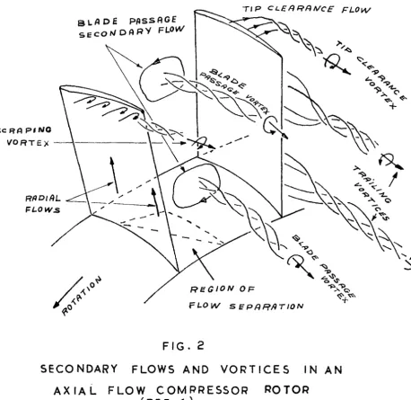
better understanding of the mechanism of the flow in the wall boundary layers is necessary to permit the development of a model of the flow which will allow the influence of these regions to be accounted for in design, and to determine the main sources of loss and the factors controlling these sources.

The flow in the end regions of a blade passage is complex. The main features contributing to this complexity are the blade passage secondary flow, tip clearance flows, effects due to rel-ative motion between moving blade rows and the stationary walls, flows resulting from radial pressure gradients and the influence of flow separation which occurs at the junction of blade suction surface and the end wall. These various influences are illus-trated in Fig. 2; a detailed discussion of each will be found in Chapter 2.

Qualitative and limited quantitative information is available on passage secondary flows and tip leal<:age effects but the flow separation originating in the corner bounded by the end wall and the suction surface of a bl~ide appears to be the major cause of loss. Data on this phenomenom are limited. In this thesis a detailed study of the boundary layer on the hub wall dovmstream. of the rotor and through the stator row of a single stage axial flow compressor is reported.

Next to the wall there is a region controlled by the wall in which the flow angle remains constant and the velocity profile can be described by a logarithmic distribution. Further from the wall the flow is dominated by vorticity generated by the turning of the end wall boundary layer and undergoes considerable over turn-ing. On the outer edge of the boundary layer a third region dom-inated by a second vortex rotating in the opposite direction to the passage vortex exists. This vortex appears to originate from a separation region similar to that found in the stator row and it contains a major portion of the losses occurring in the hub region.

Measurement of the distribution of turbulence components downstream of the rotor indicate distinct directional properties, which appear to be due to the rotor wakes. As a result a model

2. A illNI11'W OF SECONDARY FLOWS Alf.D LOSSES IN .AXIAL FLOW COMPRESSOHS

The main features controlling the flow in the hub and tip regions of a compressor are

(i ) Secondary flows set up by turning of the wall boundary layer.

(ii) The effect of separation of the wall boundary layers.

(iii) Tip clearance leakage flows.

(iv) Effect of relative motion between the end walls and rotating rows.

( v ) Flow due to radial pressure gradientil.

In this chapter these flows will be discussed and various estimates of the component losses will be reviewed.

2.1. Estimation of Losses

In an actual machine it is difficult to separate the effects and resulting losses due to each of the flows mentioned above. The system in general use is that suggested by Howell (Ref.

5)e

Howell divides the total losses occurring in a machine into three components. The drag coefficient Cn can then be expressed as

=

(1)

Howell has allowed for the annulus drag by using the relation

= 0.02 s/h (2)

This estimate is obtained by assuming a wall friction coefficient of 0.010 which is approximately twice that normally encountered in pipe flow. It is stated by Carter (hef. 6) that the high value is used to allow for adverse pressure gradients found in a compressor stage. However, as noted by Wallis (Ref. 7) in regions with adverse pressure sradients the skin friction should be reduced. The reason for Rowell's selection of this la:::'ge value can be found in Reference (S), which states in reference to cascades, that the secondary losses are negligible and the total,loss in a cascade can be accounted for by the profile loss and wall friction loss (Equation

2).

This statement has been proved incorrect by sub-sequent research (Ref. 8) and it is apparent that the annulus drag expressed by Equation (2) not only accounts for the wall friction losses but also for the considerable losses due to sec-ondary flows and flow separation which occur in cascades.

In an actual compressor Howell states that the profile and skin friction losses remain as for a cascade and introduces a sec-ondary drag coefficient,

Cns

to account for the secondarJ flow losses which are no longer considered'negligible.

= a C 2 _{1 (3)}

These two drag coefficients give a reasonable estimate of the losses occurring in the hub and tip regions of a compressor. How-ever, the simple approach cannot be expected to be accurate under all conditions particularly for off-design operation, as these relationships are a function of blade loading only, while the total losses are dependent on a large number of parameters (Ref. 4)

= f(Re, s/c, h/c, t/c, 6ic, M, ~' CL' R) (4) 2.2. Secondary Flow Due to Turning of the End Wall Boundary Layer

One of the most important sources of secondary flow in the end wall region of a blade passage results from the tu~ning of the wall boundary layer. Assuming that the static pressure is constant through the hub and casing boundary layers, in the radial direction, when this low velocity air is deflected through an angle equal to that of the main stream, the centrifugal forces developed are not sufficient to balance the pressure gradients imposed by the mainstream. Hence to maintain equilibrium the boundary layer is deflected through a greater angle giving rise to a cross flow and a resulting streamwise vorticity. This vortex will hereafter be referred to as the passage vortex.

The presence of this vorticity has been demonstrated by the flow visualization studies in cascades carried out by Herzig and Hansen (Ref.

9).

Smoke filaments showed a strong cross flow in

.An analytical method of prediction of this flow has been developed by Squire and Winter (Ref. 10). For an incompress-ible inviscid fluid with a small component of vorticity normal to the flow the secondary vo:r:tici ty W generated by tur.aing the .

s

flow through a small angle E can be expressed by

w. -

_S2

w -

_SI = - 2 dU1 E:

dy (5)

Hawthorne (Ref. 11) using a more general theory has shown that

\{ - =

SI

z

2

f

d

Pa

sin

r

d

€

pu2

I

(6)

where

Fb

is the total pressure and

'(j

the angle between the

prin-< •

ciple normal to the streamline and the surface of constant total pressure or Bernoulli surface •

.An alternative derivation of the above expression is given by Preston (Ref. 12) ; the theory has been further developed by Smith (Ref. 13) and .Marris (Ref. 14)

Various investigators have attempteQ to simplify Equation

(6) by assuming

't

=

IT /2 and W .-

=

0 but at low turning angles

SI

the difference between the results given by these more complex relationships and the simple expression of Squire and Winter, Equation (5), is small.

The velocity components induced by this secondary vortex ~5 can be obtained by introducing a secondary stream function

such that the induced velocities dmm.stream of the cascades are u2

=

·ci _~~

4Js

u3 C>lJJs

The secondary stream function then satisfies the Equation (8) Hawthorne has sho-vm that by assuming W₈1

=

0 and using Equation (5) that the change in average outlet angle through a cascade, ~d-.2 is given by the Equation

-- ·- 2 c.os d-2

11 U1 cos d-1 (9)

where u is average secondary velocity in the x direction and

(10) where

u

₁

(I\)

is the boundary layer profile •

The basis of Equation (9) is that it is assumed that there is no rotation of the Bernoulli surface. However, measurement in cascades have shmv.n that rotations of the order of 30° to

0

40 can occur. Because of this significant rotation, Hawtho:i:ne's

invisc~d model overestimates the secondary vorticity.

Horlock et al (Ref.

16)

report that the outlet angle distrib-ution found near the wall downstream of a cascade showed

over-turning near the wall and underover-turning in the mainstream but the position of maximum underturning occurred at a distance of twice the inlet boundary layer thickness from the wall. The theory predicts it to occur at a distance equal to the inlet boundary layer thickness.

The failure of the theory outlined. in this section to pre-dict the flow is due to the presence of flow separation occurring in the suction surfr.ce end wall corner of the cascade.

2.3. End Wall Boundary Layer Separation

The available data (Ref.

16

and

17)

indicate that this separ-ation is due to the ?resence of the wall and is not a direct result of the secondary flow, although the secondary flow may be a major factor affecting the condition of the wall layer.

The argument that the flow separation occurs as a result of high local lift coefficients has been disproved in the tests des-cribed above. With no wall present, tests with a local

c

1

=

1.015 at the spanwise position corresponding to the centre of the wake showed no sign of separation but with a wall present separation occurred with a local

c

1 =

0.653.

A

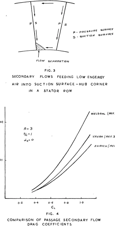
portion of the losses which appear in the region of sep-aration are crea,ted at other positions in the blade passage. The passage vortex carries low energy air from the wall boundary layer into the suction surface end wall corner and in the stator row of a machine radial pressure gradients feed low energy air from the blade boundary layers and outer casing wall into the corner. This is illustrated in Figure

(3).

The spearation does not appear to occur abruptly but grows slowly, increasing witn mainstream turning. Hanley (Ref. 18) found that the separation was primarily a function of the inlet boundary layer thiclr.ness and pressure rise through the blade row,

and states that severe separation will occur if

)

.D. p

+

o.02s5

~f

u,2

0.0185 (11) Horlock (Re.f. 16) correlates severe wall separation with passage blockage and on the information of Haller states that serious separation will occur in cascades if

coscJ...1

cos c)..'2 ~

o.

72

(12)

in the growth of secondary flows. Blade aspect ratio (A == span/chord) not only controls the relative magnitude of the effects which end wall disturbances have on the mainstream but studies by Shallaan reported in Reference (34) indicate that it also has a major influence on the form of the secondary flows.

Shallaa.n found that in low aspe.et ratio cascades (A

=

2) the flow appears to r,otate more and separation occurs further out along the blade than in higher aspect ratio (A

=

5) cascades where the separation occurs equally en the end wall and blade surface. The separation in low aspect ratio·.cascades was found to be more severe.

2.4. Passage Vortex and End Wall Separation Losses

Secondary flows resulting from the passage vortex and dist-urbances due to flow separation in the suction surface/end wall

junction are the two features controlling the flow in the end wall region of a cascade. As a result the information on these

two losses, which is purely empirical, combines the losses res-ulting from these two factors.

0

90

the loss due to complete dissipation of the kinetic energy of the secondary flow would be 0.

:c;b

and 17~ of the inlet kinetic energy compared with total losses through the bend of

5%

and

25%

respectively. This evidence that the kinetic energy of the secondary flows generated when a boundary layer region is tuined is negligible compared with the magnitude of other losses occurr-ing is supported by Mellor and Dean in the discussion of Reference (13).

From the data reviewed above, it is evident that the losses due to the second2.ry flow are negligible compared with those resulting from the end wall separation. Hence any expression derived to account for the losses must consider the parameters controlling-the wall boundary layer, it must not be based on para-meters desc1:ibing the secondary flow resulting from the passage vortex.

Meldahl (Ref. 21) has proposed the following drag coeff-icient to account for these losses.

=

0.055 C₁2 A

(13)

Vavra (Ref. 31) on the basis of a comparison of the expres-sion presented by Meldahl with that given by Howell for secondary flow losses (Eq_uation 3) claims that the coefficient is too

large and suggests the modified form

As stated in Section 2.2 the e:h.'}>ression given by Howell for the secondary flow losses only accounts for a portion of the flow losses because the annulus drag coefficient, Equation (2), also contains a component of the secondary drag losses. Vavra reasons that the coefficient should be reduced since part of the secondary flow loss is recovered. This appears to be based on the asswnption -~hat the losses are manifest as kinetic energy of the passage vortex which may be recoverable and not as a result of the flow separation which constitutes the major source of the losses. There appears to be no sound reason for the reduction in the coeffecient as suggested by Vavra.

Ehrich and Detra (Ref. 22) have obtained the following empirical relationship for the loss coefficient allowing for the transport, toward the blade suction surface, of the wall boundary layer by the passage secondary flow

= 0.1178 €

2

h/s

(1 - o.2S?h)

2

Fujie (Ref. 23) suggests the expression

0.0275 CL2 (1 + 2.9 i - id

}~

€: d

(15)

(16) where id and€ d are the design incidence and flow deflection respectively.

A comparison of the drag coefficients given in Equations (13) to (16) is made in Figure (4), for a representative set of compressor parameters.

Hanley (Ref. 18) assumed that the losses due to the passage vorticity were negligible and that the major component is due

dependent on the iltl.et boundary layer thickness and the pressure rise through the cascade. Ey assuming that the boundary layer retained its two dimensional characteristics, correlations of the outlet boundary layer thickness and a profile defining para-meter were obtained. These allow a reasonable estimate of the losses to be made, for the range of cascade geometries investig-ated, provided the inlet boundary layer thiclmess and mainstream turning angle are kno1-m.

2.5. Reduction of Effects of Passage Secondary ?low and Separation Ehrich (Ref. 24) suggGsts thE.t a reduction in the passage secondar<J flow through a cascade can be obtained by increasing the turning angle in the wall boundary layers. For flow in a cascade of twisted blades the total stream.wise vorticity at out-let is given by

2

V

L/Js

(17)

The first term on the right hand side is the secondary vorticity due to turning of the wall boundary layer and the second is that due to the vai'iation in deflection along the cascades. For comp-lete elimination of the streamwise vorticity the following equat-ion must be satisfied.

constant (18)

The expression requires an increase in the turning angle as the velocity decreases.

Martin (Ref. 25) has attempted to reduce the disturbance in the end wall region of a cascade by reducing the camber at the blade tip and hence the turning angle. The results of this investigation were not conclusivee No marked reduction in losses were reported but the wall separation appeared to be reduced considerably.

These two possible solutions are conflicting. However, the prevention of separation appears to be the main requirement for reducing losses. As a result the technique suggested by Martin would appear to be more promising.

Louis (Ref. 17) suggests the use of fillets between the blade and end wall as a method of reducing separation in machines with light blade loading ( Cos d-.i

~

O. 7) and high stagger

cos d-.2

blading. At higher loadings their use does not appear to have

I

any advantage.

When a variation in circulation₁in the spanwise direction, occurs along a blade, vorticity is shed into the mainstream from the trailing edge. In a typical compressor the magnitude of the resulting loss is small.

By assuming a linear lift distribution along the blade Tsien (Re~ 26) has obtained the following expression for the i.."lduced drag.

=

Van Karman (Ref. 27.) also assumes a linear lift distrib-ution, but neglects the interference effect of adjacent blades, and obtains the relationship

=

0.0423

(1

CLi 2 (20)

,_A_

For the range of parameters normally found in compressors Lakshminanayana and Horlock (Ref.

4)

have found that Equations

(19)and (20) give almost identical results.

Vortices will also be shed into the main stream when large

tip clearances exist resulting in leakage flows which reduce the lift at other spanwise positions. However in Reference

29,

it has been found that no lift reduction occurs at the blade tip until the clearance/chord ratio exceeds 0.06. For the range of

clearance/chord ratio normally found in turbomachinery (0.02 to 0.04) there will be no increase in the vorticity shed.

2.7. End Clearance Flows

Due to the pressure difference between the two surfaces of a blade the presence of end clearance will give rise to a leakage flow. This flow sets up a vortex which rotates on the opposite sense to the vortex set up as a result of the flow induced by turning the end wall boundary layer.

At low clearance/chord ratios tne clearance flow first resulted in a vortex sheet parallel to the tip which rolled up into a single vortex some distance away from the blade suction surface, and at an angle to the main flow. As the clearance/ chord ratio was increased, the distance from the suction surface at which the vortex formed, and the angle between the vortex and the main flow both decreased, the leakage flow eventually rolling up into a vortex as soon as the flow reached the suction surface. This behaviour can be explained by the fact that at low clearance/chord ratios only leakage flow occurs but as it is increased a portion of the main flow also passes through the gap and the resultiilg mixing reduces the leakage flow velocity and angle of the leakage vortex relative to the blade chord. Leakage results in underturning of the flow near the tip and slight over-turning at a greater distance from it. As a result of the

leake,ge vortex, spanwise flow is induced along the suction surface toward the tip.

It was found in Reference (29) that for the range of clear-ance/chord ratio normally found in turbomachinery (0.02 - 0.04), no reduction in lift occurred due to leakage flow. In this range of clearances, viscous effects have a restraining influ-ence and only a portion of the bound vorticity of the blade is shed at the tip. At larger clearances (

>

0.06) the vorticity retained at the tip drops to zero and vorticity is also shed at other spanwise positions resulting in a rapid decrease in lift.

The former considers the flow to result from the pressure difference across the gap and calculates the losses by assuming complete dissipation of the leakage flow kinetic energy.

This approach has been used by nains (Ref. 32) whose analysis has been modified by Vavra (Ref. 31) for the case of a stationary blade with a triangular pressure distribution, to obtain a drag coefficient given by

CDSC =

4J2

c

CR3

(i)

c

3/2

5

c h 1

where

c

R is a gap resistance coefficient,

c

_c a contrs,ction coefficient suitable values are CR =

o.a

and C

0 =

=

0.29

(i)

cL

3/

2

h

(21)

0.5 resulting in (22)

Shed vortex theory assumes tne leakage is induced by the vortices shed at the tip and uses lifting line concepts to calc-ulate the losses. Early investigators such as Betz (Ref. 35) assumed the lift dropped to zero in the gap, however, Lakshminar-ayana and Horlock j_~ the studies described earlier in this section have found that due to real fluid effects some lift is retained at the tip for small clearances (clearance/chord ratios< 0.06).

For the aerofoil with mid span gap Lakshminaraya.na has devised the following expression which shows good agreement with exper-imental drag coefficients·.

( 23)

For small clearance/chord ratios of the order of those found in turbomachinery (0.02 - 0.04) EQuation (23) can be

app~ox:imated by the linear relationship

=

l •

4

(1 - K) CL 2 (

1 )

s

.A

and assuming K

=

0.5 in this range O. 7 CL 2 ( 1)

T

s

(24)

(25) Meldahl (Ref. 21) suggests the empirical relationship for the losses due to leakage

CDSC

=

o.

25 ( ~) ( 1 ) 0₁2 (26)

cos ol.a

A

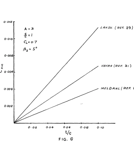
The expression given by Rains - Vavra, Meldahl and EQuation (25) are compared for a typical cascade in Figure

6.

The first two predict a considerably lower value of drag than the latter.

Shrouding of the blades has been suggested as a means of reducing the effect of tip clearance. There is little inform-ation on this aspect, but as is pointed out by Carter (Ref. 6) shrouding a blade row replaces circumferential leakage between blade passages with an axial leakage. As a result there is little to be gained.

2.8. Interaction of Leakage and Passage Secondary Flows The discussion in the previous section only considered clearance flow isolated from other influences. In this sect-ion the interactsect-ion of leakage flow with other secondary flows is discussed.

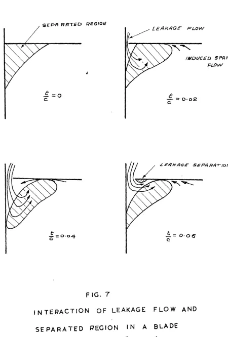
La.kshminarayana and Horlock (Ref. 29) investigated the losses resulting from leakage and cross passage flows in cascades and discovered that a controlled amount of leakage flow had a bene-ficial effect ; by reducing the severity of the separation occurring in the corner between the suction surface and the end wall the total losses are considerably reduced. For the cascade investigated the optimum clearance/chord ratio was found to be 0.04.

This behaviour is shown diagrammatically in Figure (7) based on the flow visualisation studies of Reference (29). With no clearance (a) there is a severe separation zone in the corner between the suction surface and the end wall. With a clearance gap (b) the leakage flow tends to lift the s~parated

region off the end wall. As the clearance is increased to that corresponding to the minimum loss (c) the clearance flow tends to sweep the separated region off the end wall and moves along the suction surface before rolling up into the leakage vortex, the spanwise flows induced by this vortex also tend to remove the separated region from the suction surface. When the clear-ance is further increased (d) the leakage flow rolls up as soon as it reaches the suc~i;ion surface ; the degree of interaction with the separated region is reduced, resulting in increased losses.

The mechanism described above for the reduction in losses when leakage and passage secondary flows interact is controlled by the relative magnitude of the two flows. It appears in the investigation reported in Reference 29 that the leakage flow was the dominant flow and the secondary flow relatively weak at all times.

The presence of a finite value of tip clearance at which total losses are a minimum has been reported by Dean and Hubert though this minimum is not necessarily less than the loss value at zero clearance. The information from these sources is re-produced in .F'igure ( 8) which is taken from Reference ( 29).

It is evident that if the reduction in losses resulting from the mixing of the flows in cascades described above occurs in machines, then extremely small clearances are not necessary and a finite value will give a better performance. llorlock (Ref.

34)

states that, in machines, the effect of blade rotation may reduce the optimum value of the clearance/chord ratio below that foLmd in cascades though no detailed measurements in machines are available.

The drag coefficients given in Equations (22) ai~d (25)

can be used to give a_reasonable estimate of the losses occurring in isolated leakage flow but when the:re is interation beh1-:e-en leakage and other secondary flows, as described in this section,

2 ..

9.

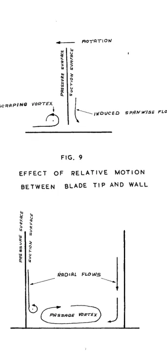
Relative Motion Between Biades and Wall

Leak.age flows occurring at the tip of a rotor are further complicated by the relative motion between the blade and wall which generates a "scraping" vortex. In the case of a compressor where the pressure surface leads, this results in a deflection of some of the air which would have passed through the tip gap, with a resulting reduction in clearance flow. On the suction

surface spam-rise flows are induced toward the wall. These flows are shown in Figure 9. The relative motion appears to increase the loading at the tip.

Howell (Ref. 2) reports that clearances up to 17"~ - 21~ of blade height appear to have little effect on losses in actual machines but at greater clearances the efficiency falls by approximately 310 for each 1% increase in clearance. This

insensitivity at low clearances may possibly be the result of the effect of the sc:r:aping vortex discussed above or the effect of the interaction of leakage and passage secondary flou discussed in the previous section.

2.10.Radial Flows

For radial equilibrium in turbomachinery radial static pressure gradientsmust exist to balance centrifugal forces. These must satisfy the equation

'2.

f

Vw

r

This results in a radial pressure gradient toward the hub. In a stator row, assuming static pressure is constant across the blade boundary layer normal to the blade, this pressure gradient will be imposed on regions in which the air has a low tangential velocity component and hence a low centrifugal force acting on it. The resulting unbalanced force will cause this air to flow toward the hub.

In a rotor the absolute tangential velocity of the air is considerably less than the blade velocity. As a result, stag-nent air relative to the rotor will have a tangential velocity component greater than that of the mainstream air and the res-u.Jl.ting higher centrifugal force causes this air to flow toward the tip.

Regions of stagnent air which may be transported by these radial pressure gradients exist in the blade suction surface boundary layer, particularly in areas such as separation bubbles and in the wake.

Flow visualization studies (Ref. 35) have shown that the radial flow on the suction surface of a stator blade forms a vortex in the end wall/suction surface corner of the blade pass-age which rotates in the opposite direction to the passpass-age vortex. This is illustrated in Figure 10. Radial flow between the tip and hub regions explains the improved conditions and in some instances the absence of secondary vortices at the tip of stator rows (Ref.

35).

If the flow disturbances near the tip are small and a suitable radial flow path is present the low energy air will be fed into the hub region rather than forming a vortex near the tip. In a rotor the direction of the radial flow is

reversed and an improvement in hub conditions can be expected.

In multi stage machines radial flows of low energy air between tip and hub regions result in a certain amount of mixing with the mainstream. In Reference (36) Hansen and Herzig state that this mixing prevents continuous grqwth of the hub and casing boundc:,ry layers and generates a more uniform radial distribution of axial velocity.

!~has been suggested that fences at mid span be used to prevent the flow of low energy air along the blade into already critical regions. These reduce the radial flows (Ref.

35),

feeding the low energy air into the mainstream but the increase in viscous losses resulting from their introduction makes any

nett improvement a debatable issue.

As the radial pressure gradient is fixed for a given design the most effective method of reducing radial flow appears to be by improved blade design this will reduce the a.rnount of low energy air available for transport, and by reducing blade

boundary layers and wake thiclmess, reduce the size of the radial flow paths.

2.11 .AnlLulus Drag

The annulus drag is equally as important as the secondary drag in the estimation of the losses in the hub and tip regions of a cascade. The annulus drag coefficient was introduced by Howell (Ref. 2) to allow for the friction losses in the end walls of a blade passage. Howell suggested the relationship

This is obtained by assuming a skin friction coefficient of 0.01 which is approximately twice that normally encountered. The reason for this high value has been discussed in Section 2.1. A more realistic expression is obtained by taking a skin f±iction coefficient of 0.005 which results in

CDA

=

0.01 s/c (28)

Vavra (Ref.

31)

recommends the expression

= 0.018 c/h (29)

The coefficient in Equation (29) was obtained by comparison with Equation ( 2) • As a result this expression also includes the portion of the secondary drag included in the Howell relationship. The form of the expression does not appear to have advantages over the simple relationship obtained using the Howell principle of considering a friction force acting on an area equal to that of the end walls of the blade passage.

2.12 Total Second.ary Flow Losses in an Axial Flow Compressor In Section 2.11 it was argued that a more realistic value for the annulus drag would be half that indicated by Howell, Equation (2), and that the remainder of the annulus drag as calculated by Howell was due to secondary flow losses. .As a result the total secondary losses using the Howell expressions will be given by

=

0.018 C

12 + 0.01 s/h

Meldahl (Ref. 21) suggests a secondary drag coefficient given by

CDS

0.055

c

₁₂

+

0.25(!)(

1 )

C12

- - c cosd.2

-A

A

(31)

In this section the various sources of secondary flow

loss in a compressor have been discussed and various expressions for the resulting drag have been presenteu. These can be

combined in the manner suggested in Reference

(4),

to give a total secondaI"J drag coefficient given by

cns

=

₊

_Cnsc

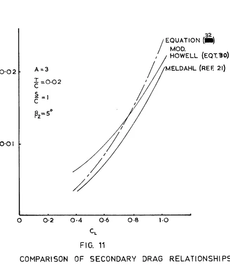
+ (32)

suitable values for the components are

=

Meldahl (Ref. 21).

Cnsc

=

_o.

_{7 CL}2 _{( i ) Lekshminarayana & Horlock (Ref.29)}

- c '

CnsT

=

,

A

0.0423 (1 - C10 ) 2 C1i

c

₁

~ Von Karman (Ref. 28)

-

A

Equation. (32) does not take account of the effect of radial flows and blade rotational influences such as scraping vortices and flows induced by centrifugal effects hut these omissions are balanced by the fact that no allowance has been made for the reduction in total losses due to beneficial interaction between the component flows as discussed in Section 2.8.

The dra.g coefficients- predicted by Equations (30), (31) and (32) are shown in Figure 11 for a representative compressor geometry. It is evident from Figure 11 that, for a typical compressor, the three expressions give similar values. As a result there is little value in using the more complex

2.13.Concluding Remarks

The information which has been presented in this section has been obtained almost entirely from studies of two dimen-sional cascades and isolated aerofoils. The data on losses has been obtained from detail measurements in cascades and from losses inferred from efficiency calculations on machine tests. No detailed measurements have been made in machines with the aim of describing the mechanism of the flow directly rather than inferring what might be from other evidence.

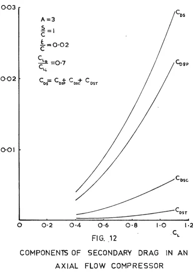
From the work which has been carried out on two dimen-sional cascades, models exist for seconcle,ry flow originating from the passage vortex when removed from end wall effects (Ref. 15) and for tip clearance flow when removed from other influences (Ref. 29). However a study of the components of the secondary drag coefficient given by Equation (32), shown in Figure 12, indicates that the major portion is due to CDSP' the greater part of which results from flow separation in the suction surface/end wall corner of the blade passage. The

info~mation available on the mechanism of this latter phenom-enom is small, though the extent of the separation does appear to be influenced by the history of the wall boundary layer and by the loc~d on the blade row (Ref. 18).

A second factor of importance in a machine is the effect of interaction of the various secondary flows. It appears that the nett loss in a machine may be less than the sum of the losses due to individual flows (Ref. 29), but at present no

3.

EQ,UIP.i:Vff.:J.'l"T AND IWSTflffivIENTATION

3.1.

Vortex Wind Tunnel

The work described here was carried out on the Vortex Wind Tunnel at the University of Tasmania. The experimental rig shown in Figure

13

is a sintsle stage axial flow compressor cont-aining three blade rows, namely, inlet guide vanes, rotor and stator. A brief description of the rig is given below. A

more detailed description, together with a su.mmaI."J of previous work carried out is given by Oliver (Ref.

9).

The major dim-ensions of the machine are listed in Appendix A.

Air enters the tunnel radially and is turned through 90° with a contre.ction of

7

to 1 into a

45

inch diameter aluminium section one diameter in length containing the three blade ro1·1s. This is followed by a

13

feet,

7°

included angle diffuser with a cylindrical core which is flared out to give a radial exit. The exit opening is controlled by a cylindrical throttle giving an opening from zero to 30 inches.

The blades are

9

inches long and have a

3

inch chord giving an aspect ratio of

3.

The hub/tip ratio is

0.6.

There are 38 blades in the tw·o stationary rows and 37 in the rotor giving mid blade hei6ht space/chord ration of 0.99 and 1.02 respectively. The blade row centres have an axial spacing of two chord length~.

The blading has a circµlar arc camber line clothed with a C. 4 profile with a thicimess/ chord ratio of lO~b. The blades are twisted about a radial straight line through the middle of the camber lines of all sections. They are designed on the basis of the Howell data to give nominally free vortex conditions at the design duty (~

=

0.8) with

50%

reaction at mid blade

The tunnel may be split at flanges on the centre line and between each blade row allowing the inlet and required portion of the outer casing to be rolled back to provide access to the blades. The stationary blade rows are mounted on rin:::;s, which " can be rotated. through a circumferential distance of two blade

spaces thus allowing the blades to be traversed. past a

station-ax~ measuring probe. Blade clearance at the hub is approx-imately 0.04 inches i.e. 0.51; of the blade height.

The rotor is driven by a 40 horse power electric motor controlled by a Ward Leonard set, maximum speed is 750 R.P.M. which corresponds to a blade chox·d Re;ynolds number of 2 x

10~

based on blade speed at mid span.

The rotor speed is set by a stroboscope triggered by a 100 cycle signal from a crystal clock and is monitored by use of a photo electric cell arr~nged to give one pulse per revel-ution with counting on a decade counter over a period of one

• J..

ffil.UUue. The result is then displayed for one minute and the

cycle repeated the minute intervals are also timed by the crystal clock. This method·enables the speed to be maintained within + 1 R.P.M. i.e. + 0.2j~.

Instrument slots are fitted on the horizontal diameter between the blade rows. Probes are mounted in a chuck fitted to the tunnel side allowing movement in the axial and radial directions and rotation of the instrument on its horizontal axis. The axial position can be set using a vernier scale to an accur-acy of 0.01 inch. The radial position is controlled by a micro-meter screw, when working near the wall (particularly when using hot wire probes) a dial gauge (0.0001 inch/division) was used. The angular position of the probe is controlled by a micrometer

0

Pressure measurements were made on a multitube manometer inclined at a slop:i of one in four. The working fluid was methyl alchol the specific gravity of which ·was taken as 0. €30 and constant. A ":Betz" projection manometer was used during calibration of the various probes.

3.2.

Hot Wire Anemometer

Hot wire measurements were made using a "Disa11

55

_AOl

constant temperature anemometer in conjunction with probes constructed at the University of Tasmania. These consisted of 000003 inch diameter tungsten wire approximately 0.1 inch long welded to nickel prongs 0.03 inches in diameter and

i

inch in length. It was suspected that this long length of prong could have introduced a vibration problem. The effect of vibration o:f the probe and supports is always an unlmovm :factor but normally this produces peaks in the turbulance components where the exciting frequency corresponds to the natural frequen-cies of the wire and its supports, no such peaks were discerned in the readings obtained during this investigation.

The wires were calibrated in an open circuit wind tunnel where velocity was measured using a pitot static tube connected to a ":Betz" micro-manometer. The turbulance level in the tunnel was approximately

2%.

11_{he hot wires were used to measure mean velocity,}

turb-ulance components and flow direction. The turbulance

comp-1

onents were obtained using the method presented by Hinze (Ref.

The directional sensitivity of the wire to flow direction was used when measuring flow angle. The D.C. voltage changes with angle in the manner shown below.

(35) When the wire is nearly normal to the flow the variation with

angle is small but at ~

45°

the sensitivity is sufficient to

0

set angle for a given voltage repeatedly to better than

0.25 •

The method used to obtain flow direction was to select a voltage at approximately

45°

to the direction of the flow, find the two angles corresponding to it and bisect them to give the flow direction.

Although this method of measuring angle was rather tedious there seemed to be no alternative in the presence of blade wakes from the rotor row which were known to give misleading readings on yressure probes. The non linear effects of the high turb-ulance levels within the blade wakes probably also upset the hot wire readings but this source of error is thought to be small.

The datum for angle measurement was obtained by attaching a cross bar to the probe holder and measuring the angle between the bar and wire with the equipment shown in Figure

14.

The horizontal position of the bar was recorded a..nd the probe

rotated until the wire Has horizontal. rrhis was determined by the cross ~irof the level, or rather by traversing one end of the cross hair along the wire. The angle between the

0

of the form

dE ' _{-· iE d-.Radt/(R - R )}

w a

where d... is the thermal coefficient of resistivitye

E the measured voltage

R wire resista.nce at ambient temperature a

R operating wire resistance

w

was applied to all voltages measured.

(36)

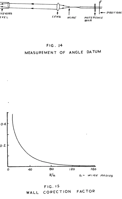
When operating a hot wire close to a wall the heat loss to the boundary introduces errors as also does the change in flow pattern around the wire due to the proximity of the wall. Little information is available on this problem, the most recent is that of Wills (Ref. 38) whose method has been used in this investigation.

Wills applies his correction by subtracting a number K from

w

the value of R

o.

45

where R is the wire Reynolds number

ew ew

based on the wire diameter. The value of K de_pends on the w

distanre from the wall as sho1m in Figure

15.

The correction factor was obtained for laminar flow. For turbulent flow a value of approximately half this is sug:;Sested by Wi~ls and this

recommend~"tion, in absence of better d2~ta has been used in this thesis.

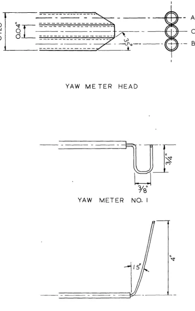
3.3. Cobra Yaw Meter

The cobra yaw meters sh01m in Figure 16 were used for measuring total pressure, velocity and flow direction through and do~mstream of the stator. They consist of three one millimeter tubes arranged in the form of an arrow head, the

0

two side tubes being cut off at an angle of

35

to the probe

Instead of the usual method of nulling the two side hole readings to obtain direction and using a factor on the differ-ence between side and centre readings to give velocity, the probes were calibrated for use in the yawed position. This reduces the time required to obtain data and enables the probe

'

to be placed in positions not otherwise possible. The amount of work required in calculation of results is increased consid-erably but with the use of computer this is not a major conse-quence.

The derivation of the relationships Given below, used to calibrate the probes, can be found in Appendix C.

The angle from null,0-. , can be determined from the pressures in the three tubes by the relationship

hA h _{c = F( d-- ) (37)}

113

h c

the velocity from either of the two relationships

u

=

I

_{2g(hA he)}

I

.1. ( J.. )

201

=

I

_2g(113

_he)

I

_{·2a_}

1 '

2

{ °' )

(38) and the difference between true total head and the centre tube readfugby

h

0 h c

=

U

2

H (d.. )

2g

(39)

Where F, G

1, G2 and H are functions of c:J... , the angle from the

null position.

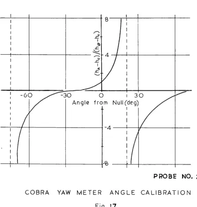
The design of the wind tunnel made probe number 2 necessary for measurement through the stator. Becasue of the shape of the blade passage and high crass flows in regions of flow separation the probe was at times operating at large angles from the null position. For this reason the probe was calibrated through a 1 _{arge range,}

_:!:

1000. _{In the ordered regions of flow (away}

from the blade walls), the probe was kept as close to null as possible but due to the fact that rotation of the probe chsnged the axial position of the measuring station it was not usually operated as close to null as was probe 1. The accuracy outside the range

!

15° is doubtful but the probe measurements enable an order 6f· magnitude to be obtained where as no information would otherwise have been available.

The calibration of meter No. 2 against yaw, shown in Pigure

17,

was carried out at velocities varying between 20 and 100 f.p.s. but no variation with Reynolds number was detected.

I '1'2

For the velocity calibration

U/

f !Jh] against d-..

Figure 18, whereLJh is the difference between the centre and one side hole, the difference between the same pair of holes could i.mve been used throughout butLlh was taken as the largest of the two head differences to avoid errors in using small differences of large numbers.

The total head correction is shown in Figure 19. For

:!:

4°

from null the centre hole reads true total pressure within

3.4.

Factors affecting Pressure Probes

When a pressure probe is used i:a. a boundary layer allowance must be made for the effect of

(1) proximity of the wall

(2) the trai.""lsverse velocity gradient (3) turbulence

and if the probe is used in' a turbo-machine

(4) the influence of the wakes of upstream blade rows.

Yiacmillan (Ref. 39) states that the wall has an influence when the probe is closer than two diameters from it and suggests that this can be accounted for by adning an increment to the velocity measured varying exponentially from 1. 55'~ when the probe is on the wall to zero when the probe centre line is two diameters away.

The effect of the transverse velocity gradient can be expressed as a displacement of the effective centre of the tl,lbe toward the region of higher velocity. The apparent increase in velocity is roughly proportional to the velocity gradient with the result that the displacement is approximately constant. Young and Maas (Ref. 40) have suggested for squRre cut tubes the relation-ship

L1 ~

D = 0.13 + 0.08 d D

(40) where ~ y is the effective displacement, D the probe outer diam-eter and d the probe inner diamdiam-eter. However, later uork. ·, by Macmillan (Ref 39) suggests that the above relationship over-estimates the displacement and a. more accurate result is given by

This would decrease the velocity indicated by the col::Ta probes when touching the wall by approximately 21~ and by 0.8% when 0.05 inches from it.

The correction for wall proximity ro1d that due _to shear act in opposite directions. Combining the two the nett result·_ is small, less than l)ia. As the information given above is for pitot tQbes i.e. a single tube probe, ai1d that the effects on multitube probes have not been investigated, it was considered

that no improvement in accuracy would be obtained by applying corrections .for these influences.

The ef l'ect of turbulence is to increase the pressure indic-ated by the probe by

-?zp

uf

where u

1 is the fluctuating

compon-ent of the velocity in the direction of the probe. No hot

wire measurements were taken through and donwstream of the stator. However, at ~ inch upstream of the stator leading edge the

maximum value of

if

u

12 in the bmmda.ry layer was 1.47~ of the local dynamic head.

Measurements in turbo machines downstream of rotors have shown effects of a greater magnitude than those indicated by the classical corrections mentioned above.

In Fig. 20, total pressure measurements in the flow down-stream of rotor in the Vortex Wind 'l1_{u.11nel, repon.teO. in (Ref.}

41)

are show.a. The total pressure

i

inch from the rotor trailing ede;e is approximately

50%

greater than that measured at l i inches. The difference is approximately constant across the armulus and can not be explained as a boundary layer effect. In Fig. 21, the measured mid span total pressure is plotted as a ftmction of distance from the rotor. ~he pressure drops

A similar occurrence has been noted by Wallis (Ref. 7) who reported that measurements near the trailing edge of the rotor in an axial flow fan gave total head rises which when used to calc-ulate efficiencies gave unreasonably high values. Wallis also found the excess in total pressure to be approximately constant across the fan annulus. Neustein (Ref.

42)

also reports high values close to the trailing edge of a rotor.

The cause of these errors cannot be accounted for by the effects mentioned earlier in this section and appear to be due to the rotor blade wakes. No satisfactory explanation of this phenominom is available.

In this investigation pressure probes were not used in the region adjacent to the rotor but were employed through and downstream of the stator. Efficiencies calculated from pressure measurements l?J- incl-.es from the :rotor trailing edge appear to be no more than 1% high. Allowing for a further decrease

4.

THE HUB BOIDl:D.ARY LAYER THROUGH 'Elli STA'l'OR 4.1. Experimental Procedures

The boundary layer on the hub thxough and dovmstream of the stator row was studied using the cobra yaw meters descri1)ed in Section

3.3.

The distributions of velocity, total pressure and flow angle were measured at 0.5 inch (0.167 chord J~engths) intervals through the blade passage and at 0.5 and 1.5 inches (0.167 and 0.50 chord lengths) downstream of the trailing edge.

These measurements were carried out at a duty s:pecified by a flow coefficient ~ =

o.

75 and pressure coefficient

lJl

= O. 70 corx·esponding to a rotor speed of 500 R.P.M. and 8 inch throttle setting. This is close to the blading design point (~

=

a.so

and

l/J

= 0.64).

Measurements were taken at radial spacings varying between 0.025 inches near th~. wall to 0.5 inches in the mainstream. The probes were placed at the reg_uired re.dial distance from the wall and the blade row rotated past the stationary probe. The

distance between readings in the circumferential direction varied between 0.1 and 0.3 inches.

4.2. Experimental Resul~s

4.2.lTotal Pressure

The feature of these plots is the growth of the region of separation in the suction surfaco/hub wall corner. A region of separation is already present at

0.167

chord lengths from the leading edge (.Fig. 22). The region grows as it passes through the row and the contours suggest a radial movement of the low energy core from the hub surface to the blade surface ..

Downstream of the trailing edge the low energy core appears to diffuse and move away from the wall, and relative to the blade wake in the mainstream is displaced away from the side of the wake originating on the suction surface of the blade.

4.2.2.Velocity

Representative velocity distributions are presented in Figs.· 29 to 31. These show the same basic feature of a low energy region f onning and being dis~laced from the hub des-cribed in the previous section. The distribution at 0.5 chord lengths downstream from the trailing edge (Fig. 28) indicates that the flow in the low energy anre strengthens rapidly.,

Flow angle distributions at and downstream of the trail-ing edge of the blade row are shown in Figs. 32 to 34.

4.3.

Vorticity

Vorticity components in the radial>streamwise and normal to

stream~·rise directions were calculated using the relationships given in Appendix D. These are shown in Figures

35

to

37.

These components are relative to a local mean flow direction at each point.

The distribution of vorticity normal to the streamline

indicates two main regions of vorticity of opposite sign, one near the wall and the second some distance out. The streamwise comp-onent indicates one dominant vortex with a centre approximately 0.2 inches from the wall. The radial vorticity component, Figure

36,

shows a vorte)i sheet assoc:Ut ted with the blade wake. The radial vorticity generated as a result of the flow separation is smaller than that generated by the blade wake.

4.4.

Discussion

The dominant feature of the boundary layer in the stator row is the separation region which occurs in the suction surface/hub corner of the blade passage.

Leakage flow transports the low energy air from the corner in the manner discussed in Section 2.8. Initially, gro~~h

When the total pressure and flow angle distributiorsat 0.167 chord lengths from the trailing edge are superimposed

(Figure 38) it can be seen that the region of overturning corresponds with the upper side of the low energy zone and the region of highly underturned air, which results from the tip clearance flow, corresponds to the lower portion of this zone. It would appear that the leakage flow influences the rotation of the low energy region creating a streamwise vortex. The centre of the dominant streamwise vortex shown in the

vorticity plots coincides with the centre of the low ener~J core.

The vortex described above rotates in the opposite direction to that ·which woul!i be set up by the seconda:l:"J flow resulting from the turning of the boundary layer through the blade row. Dm-mstream of the trailing edge there is a region of streamwise vorticity (Figure 37) of the opposite sign to that of the main vortex near the wall and another on the outer edge of the main vortex. These are possibly induced by the vortex resulting from the interaction of the separation and leakage flow. There is no evidence in either the angle or vorticity distributions of the formation of a major passage vortex resulting from the turning of the hub boundi;i.ry layer. This could result from the fact

In the stator row studied the direction of the separation vortex is controlled by the direction of the leakage flow. In general the direction of rotation of the voi·tex generated in this region will depend on the interation of a number of forces. In the case of a blade row with no clearance flow and a high passage cross flow resulting from turning the wall bom1dary layer it would be expected that the vortex would rotate in the opposite direction to that reported above.

The two regions of normal vorticity of opposite si15n result from the forrii of the boundary layer. Due to the leakage flow the boundary layer in the region of the s_epar-a tion core ts_epar-akes the form shown in Pig.

39

with a velocity peak near the wall decreasing thi·ough the low energy core

5.

THE rIUJ3 BOUNDARY LAT.l'.ll BETWE:t.l'J THE ROTOR AND STATOR 5.1. Experimental Procedure

Detailed measurements of the hub boundary layer between the rotor and stator rows were made using the hot wire anemo-meter described in Section 3.3. The mean velocity, flow direction, the root mean square value of the velocity fluct-uation along and normal to the flow direction and the turbu-lence cross product in the axial-tangential plane were measured. The measurements were ca~ried out at the same loading as for measurements through the stator reported in Section

4.

Five radial traverses were made at half inch axial inter-vals i.e. 0.167, 0.333, 0.50,

o.667

and

o.s33

chord lengths, from the rotor trailing edge. The radial spacing between measurements was varied according to the rate of change of the parameters, varying from 0.001 inch near the wall to 0.5 inch outside the boundary layer. The wall position was determined by connecting an avometer between the tunnel wall and the probe and moving the probe in until contact was just made. Using a dial gauge the wall position could be determined to approx-imately 0.0005 inches. To detect any errors in calib~ation

resulting from touching the wire on the wall, the wire was recalibrated after each set of measurements.

5.2. Experimental Results. Velocity

The maan velocity distributions are shown in Figu:ce 40. The velocity profiles are orderly to a dista..~ce of approximately 0.3 inches from the wall. (Blade chord = 3 inches, blade

1.25 inches from the wall. The outer limit

of

the bounde,ry layer is difficult to define in a manner similar to that used for two dimensional boundary layers due to the mainstream velocity variations resulting from spanwise blade loading effects.

ATI.ogarithmic plot of velocity, Figure

41,

iniiicates that from approximately 0.01 inches to 0.1 inches from the wall the distribution can be described by a relationship of the form

I

*

u

: : --

103

~

+

B

₍₄₂₎

-u,.

K

where B and K are constants.

u;f'

( ; )

~2

and

_Lo

is the wall shear stress.

The shear gradients near the wall are large. It was not possible to obtain sufficient points close to the wall to define the wall shear stress. Differentiation of Equation (42) with respect to y gives the following relationship.

Q~

-K

(43)

From the measurements the value of ti~ff was found to be a constant for all axial stations, with a value of approxim.-ately

9.5,

indicating that if K is a constant the wall shear stress is constant in this region.

5.2.2.

Flow Direction

The variation in flow direction through the boundary layer is shown in Figure

44.

The dominant feature is the conventional overturnir.g near the wall and associated under-turned region a further distance out. There are however, two other regions of importance. Extending to approximately O.l inches from the wall i.e. in the region in which the velocity distribution is logarithmic, there exists a region in which the flow angle remains constant. This region extends to the wall near the rotor but as the stator is approached there is evidence of a reduction in the angle close to the wall. The :flow angle in this region decreases, as shown in Figure

43,

with axial distance from the rotor. The second region lies between 0.4 and 1.2 inches from the wall where the flow is again overturned.

5.2.3.

Turbulence Components

Axial - Tangential Cross Product

The distribution of the turbulence cross product in the axial tangential pla.~e is sho~in. in 2ibure

45.

The shear stress increases almost linearly through the logaritbmic velocity region from a wall value close to zero reaching a maximum at the outer limit of the los region. The distance of this maximum from the v.rall increases with distance from the rotor, varying from 0.085 :inches 0.16 chord lengths, from the rotor trailing edge to 0.120 inches near the st'ator leading edge. The peak: value reduces rapidly with distance from the rotor, the maximum value near the stator leading edge being only

30%

of the value near the rotor.

In the region of high shear stress further from the wall the reduction is more rapid, clear definition of the peak disap:pearing within half a chord length from the rotor trail-ing edge.

R.N.S. Velocities

The root mean square value of the turbulence fluctuation$ in the streamwise direction 'is-- plotted in Figure

46.

The distribution is similar to that of the cross product discussed above. There are two regions of high turbulence, one near the wall and the other at approximately 0.6 inches from the wall, though the demarcation between the two zones is not marked as in Figure

45.