Comparing Cyber Defense Alternatives Using Rare-Event Simulation Techniques to Compute Network Risk

(1)

Rochester Institute of Technology

RIT Scholar Works

Theses

5-2018

Comparing Cyber Defense Alternatives Using

Rare-Event Simulation Techniques to Compute

Network Risk

Alexander Leon Krall

[email protected]

Follow this and additional works at:https://scholarworks.rit.edu/theses

This Thesis is brought to you for free and open access by RIT Scholar Works. It has been accepted for inclusion in Theses by an authorized administrator of RIT Scholar Works. For more information, please [email protected].

Recommended Citation

(2)

Comparing Cyber Defense Alternatives Using

Rare-Event Simulation Techniques

to Compute Network Risk

by

A Thesis Submitted in Partial Fulfillment of the Requirements for the Degree of Master of Science

in Industrial & Systems Engineering

Supervised by

Professor Michael E. Kuhl

Department of Industrial & Systems Engineering Kate Gleason College of Engineering

Rochester Institute of Technology Rochester, New York

May 2018

Approved by:

Michael E. Kuhl, Professor

Thesis Advisor, Department of Industrial & Systems Engineering

Shanchieh J. Yang, Professor

Committee Member, Department of Computer Engineering

Katie McConky, Assistant Professor

(3)

Thesis Release Permission Form

Rochester Institute of Technology Kate Gleason College of Engineering

Title:

Comparing Cyber Defense Alternatives Using Rare-Event Simulation Techniques to Compute Network Risk

I, Alexander Leon Krall, hereby grant permission to the Wallace Memorial Library to reproduce my thesis in whole or part.

(4)

Acknowledgments

This effort is supported in part by the National Security Agency under grant number

(5)

Abstract

Comparing Cyber Defense Alternatives Using Rare-Event Simulation Techniques to Compute Network Risk

Supervising Professor: Michael E. Kuhl

Vulnerabilities inherent in a cyber network can be exploited by individuals with

ma-licious intent. Thus, machines on the network are at risk. Formally, security specialists

seek to mitigate the risk of intrusion events through network reconfiguration and defense.

Comparison between configuration alternatives may be difficult if an event is sufficiently

rare; risk estimates may of be questionable quality making definitive inferences

unattain-able. Furthermore, that which constitutes a “rare” event can imply different rates of

occur-rence, depending on network complexity. To measure rare events efficiently without the

risk of doing damage to a cyber network, special rare-event simulation techniques can be

employed, such as splitting or importance sampling. In particular, importance sampling

has shown promise when modeling an attacker moving through a network with intent to

steal data. The importance sampling technique amplifies certain aspects of the network in

order to cause a rare event to happen more frequently. Output statistics collected under

these amplified conditions must then be scaled back to the context of the original network

to produce meaningful results. This thesis successfully tailors the importance sampling

methodology to scenarios where an attacker must search a network. Said tailoring takes

the attacker’s successes and failures as well as the attacker’s targeting choices into account.

The methodology is shown to be more computationally efficient and can produce higher

(6)

List of Tables

4.1 Impact Heuristic . . . 27

4.2 CVSS Categorization Values . . . 28

4.3 CVE-2009-0658 Probability Scoring Example . . . 29

4.4 Interest Rating . . . 29

5.1 Service CVSS Categorization . . . 36

5.2 Impact Assignments . . . 39

5.3 Depth - Risk Reduction . . . 60

5.4 Breadth - Risk Reduction . . . 60

C.1 Convergence - Depth - Base Case - Number of Trials . . . 83

C.2 Convergence - Depth - Base Case - Likelihood & Variance . . . 83

C.3 Convergence - Depth - Modify Connection - Number of Trials . . . 84

C.4 Convergence - Depth - Modify Connection - Likelihood & Variance . . . . 84

C.5 Convergence - Depth - Move Connection - Number of Trials . . . 84

C.6 Convergence - Depth - Move Connection - Likelihood & Variance . . . 85

C.7 Convergence - Depth - New Machine - Number of Trials . . . 85

C.8 Convergence - Depth - New Machine - Likelihood & Variance . . . 86

C.9 Convergence - Depth - Public to Private - Number of Trials . . . 86

C.10 Convergence - Depth - Public to Private - Likelihood & Variance . . . 87

C.11 Convergence - Breadth - Base Case - Number of Trials . . . 87

C.12 Convergence - Breadth - Base Case - Likelihood & Variance . . . 88

C.13 Convergence - Breadth - Modify Connection - Number of Trials . . . 88

C.14 Convergence - Breadth - Modify Connection - Likelihood & Variance . . . 89

C.15 Convergence - Breadth - Move Connection - Number of Trials . . . 89

C.16 Convergence - Breadth - Move Connection - Likelihood & Variance . . . . 90

C.17 Convergence - Breadth - New Machine - Number of Trials . . . 90

C.18 Convergence - Breadth - New Machine - Likelihood & Variance . . . 91

C.19 Convergence - Breadth - Public to Private - Number of Trials . . . 91

C.20 Convergence - Breadth - Public to Private - Likelihood & Variance . . . 92

(9)

C.22 Static - Depth - Modify Connection - Likelihood & Variance . . . 94

C.23 Static - Depth - Move Connection - Likelihood & Variance . . . 95

C.24 Static - Depth - New Machine - Likelihood & Variance . . . 96

C.25 Static - Depth - Public to Private - Likelihood & Variance . . . 97

C.26 Static - Breadth - Base Case - Likelihood & Variance . . . 98

C.27 Static - Breadth - Modify Connection - Likelihood & Variance . . . 99

C.28 Static - Breadth - Move Connection - Likelihood & Variance . . . 100

C.29 Static - Breadth - New Machine - Likelihood & Variance . . . 101

(10)

List of Figures

3.1 Splitting Technique . . . 10

4.1 IS Methodology Flowchart . . . 16

4.2 Model Implementation Structure . . . 22

4.3 Depth-Based Machine Selection Example . . . 26

4.4 Breadth-Based Machine Selection Example . . . 26

5.1 Network Example - Base Case . . . 34

5.2 Network Example - Modify Connection . . . 37

5.3 Network Example - Move Connection . . . 37

5.4 Network Example - New Machine . . . 38

5.5 Network Example - Public to Private . . . 38

5.6 Convergence - Depth - Base Case - Computational Savings . . . 40

5.7 Convergence - Depth - Base Case - FILES Likelihood . . . 41

5.8 Convergence - Depth - Base Case - DB01 Likelihood . . . 41

5.9 Convergence - Depth - Base Case - DB02 Likelihood . . . 42

5.10 Convergence - Depth - Base Case - STORAGE Likelihood . . . 42

5.11 Convergence - Depth - Base Case - FILES Variance . . . 44

5.12 Convergence - Depth - Base Case - DB01 Variance . . . 44

5.13 Convergence - Depth - Base Case - DB02 Variance . . . 45

5.14 Convergence - Depth - Base Case - STORAGE Variance . . . 45

5.15 Convergence - Breadth - Base Case - Computational Savings . . . 46

5.16 Convergence - Breadth - Base Case - FILES Likelihood . . . 47

5.17 Convergence - Breadth - Base Case - DB01 Likelihood . . . 47

5.18 Convergence - Breadth - Base Case - DB02 Likelihood . . . 48

5.19 Convergence - Breadth - Base Case - STORAGE Likelihood . . . 48

5.20 Static - Depth - Base Case - FILES Likelihood . . . 49

5.21 Static - Depth - Base Case - DB01 Likelihood . . . 49

5.22 Static - Depth - Base Case - DB02 Likelihood . . . 50

5.23 Static - Depth - Base Case - STORAGE Likelihood . . . 50

(11)

5.25 Static - Breadth - Base Case - DB01 Likelihood . . . 51

5.26 Static - Breadth - Base Case - DB02 Likelihood . . . 52

5.27 Static - Breadth - Base Case - STORAGE Likelihood . . . 52

5.28 Configuration Likelihood Comparison - Depth - STORAGE . . . 54

5.29 Configuration Likelihood Comparison - Depth - DB01 . . . 54

5.30 Configuration Likelihood Comparison - Depth - DB02 . . . 55

5.31 Configuration Likelihood Comparison - Depth - FILES . . . 55

5.32 Configuration Likelihood Comparison - Breadth - STORAGE . . . 57

5.33 Configuration Likelihood Comparison - Breadth - DB01 . . . 57

5.34 Configuration Likelihood Comparison - Breadth - DB02 . . . 58

5.35 Configuration Likelihood Comparison - Breadth - FILES . . . 58

5.36 Additional Trials Required - Depth . . . 61

5.37 Additional Trials Required - Breadth . . . 61

5.38 Standard Simulation - Depth - Comparison - STORAGE . . . 62

5.39 Standard Simulation - Depth - Comparison - DB01 . . . 62

5.40 Standard Simulation - Depth - Comparison - DB02 . . . 63

5.41 Standard Simulation - Depth - Comparison - FILES . . . 63

5.42 Standard Simulation - Breadth - Comparison - STORAGE . . . 65

5.43 Standard Simulation - Breadth - Comparison - DB01 . . . 65

5.44 Standard Simulation - Breadth - Comparison - DB02 . . . 66

5.45 Standard Simulation - Breadth - Comparison - FILES . . . 66

A.1 Convergence - Breadth - Base Case - FILES Variance . . . 72

A.2 Convergence - Breadth - Base Case - DB01 Variance . . . 73

A.3 Convergence - Breadth - Base Case - DB02 Variance . . . 73

A.4 Convergence - Breadth - Base Case - STORAGE Variance . . . 74

A.5 Static - Depth - Base Case - FILES Variance . . . 74

A.6 Static - Depth - Base Case - DB01 Variance . . . 75

A.7 Static - Depth - Base Case - DB02 Variance . . . 75

A.8 Static - Depth - Base Case - STORAGE Variance . . . 76

A.9 Static - Breadth - Base Case - FILES Variance . . . 76

A.10 Static - Breadth - Base Case - DB01 Variance . . . 77

A.11 Static - Breadth - Base Case - DB02 Variance . . . 77

A.12 Static - Breadth - Base Case - STORAGE Variance . . . 78

B.1 Standard Simulation - Breadth - Comparison - DB01 . . . 79

(12)

B.5 Standard Simulation - Breadth - Comparison - FILES . . . 81

(13)

Chapter 1

Introduction

In an increasingly digitized world, the need for secure systems has become a paramount

concern. Every cyber network has inherent vulnerabilities, which can be exploited by

ma-licious agents. The modern cyber-attacker has various scopes of intent: some seek to steal

protected data while others may simply want to demonstrate their prowess. Additionally,

hacking may be fueled by a political agenda; such a practice is known as hacktivism.

Re-gardless of their motivation, the cumulative actions of all attackers result in outstanding

financial loss. For example, time must be taken to fix damaged systems, intellectual

prop-erty can be stolen and distributed, etc. To mitigate these financial impacts, security

spe-cialists actively work to protect their networks. Thus, spespe-cialists and cyber-attacks are at

odds with each other in a battle of wits. The ensuing conflict results in the application of

complex tactics and stratagem as each side attempts to gain the upper hand [21]. One of

the possible outcomes of these struggles is that an attacker fulfills their intent, which will

affect the targeted institution. The National Institute of Standards and Technology (NIST)

represents the synthesis of an adverse impact and its associated likelihood of occurrence as

network risk. More formally, risk measures the extent by which an entity is threatened by

a potential circumstance or event [17].

Overall, the implied goal of a security specialist is to minimize network risk to the

greatest degree possible. Such a feat can be done by making changes to a networks

(14)

the set of actions available to an attacker. To this end, being able to decipher a network’s

relative risk provides much needed context to an IT specialist when faced with a variety of

(15)

Chapter 2

Problem Statement

A cyber network topology has the potential to be highly complex. Machines on the network

may be highly interconnected or buried several layers beneath public visibility. Given such

a network, there may be numerous opportunities to bring malicious intent to fruition. For

example, a network can simultaneously be vulnerable to a worm attack or data theft. Within

the scope of data-theft, there may be multiple databases to consider, each with their own

associated risk of unauthorized data exfiltration. The difficulty in determining the risk of

each data-theft event has the possibility to scale with a networks complexity. An additional

layer of stochasticity becomes apparent when considering an attackers approach to

com-promising a network. Different attackers may utilize different strategies to move between

machines on a network. Thus, manually determining the risk of various events may become

time consuming and invoke additional expenses. Manual determination of risk would

in-volve leveraging real attacks on the network. Any damage done to a network in the midst

of testing would need to be repaired. To this end, an analytic technique for determining

network risk is much preferred. Said risk tool should be able to handle the aforementioned

sources of stochasticity while providing an efficient and cost-effective means of analyzing

a network. The potential benefits of an analytic risk calculation tool will be addressed by

this thesis.

The first thesis objective concerns the development of an analytic risk calculation

(16)

interest. For the purposes of this investigation, events of interest will be limited to the scope

of attackers achieving machine access. The technique should be placed into an abstract

framework that is compatible with a variety of cyber network topologies. Since likelihood

and impact are pertinent to the calculation of risk, the design objective of the framework

will be to determine each of these metrics.

The second thesis objective entails implementing the theoretical framework. Realistic

and complex network topologies should be fed into the model during testing. To satisfy the

requirement of a complex system, subnets within the larger network should have machines

that are highly interconnected. Doing so should ensure that the framework is functional

and suitable for general usage. Depth and breadth-based search methods are two divergent

network movement techniques that can be utilized by attackers and should be investigated.

Additionally, the effects of network reconfiguration alternatives should be explored. These

alternatives could include the addition of new machines and the removal of connections.

The model should be developed as custom-made software.

The third, and final, thesis objective surrounds experimentation. Two contrasting

meth-ods should be used to validate the benefits of the model framework against standard

pro-cedures. The first method should involve a static number of trials. Under this validation

method, the confidence intervals of the risk output can be compared to determine which

procedure produces estimates of higher quality. The second validation method should

as-sess the number of trials needed to converge on an estimate of predetermined quality. The

number of trials required for convergence for each procedure indicates the required

com-putational effort required. Thus, the procedure that requires fewer trials is the procedure

(17)

Chapter 3

Literature Review

This section discusses the relevant related work on network risk, risk reduction, and

rare-event simulation. The section opens by providing additional depth to the notion of risk.

Following this discussion, focus is placed on means to mitigate a network’s risk.

After-wards, rare-event simulation techniques, as they pertain to risk reduction, are explored.

The section closes with an analysis of the various techniques.

3.1

Network Risk

Risk is considered to be the synthesis of the likelihood and impact of an event. Each of these

two constituents have their own unique qualities to consider. However, additional measures

may be recorded alongside risk. McQueen et al. [11] identify the time to compromise a

target as a potential metric to track since it represents a measure of effort expended by an

attacker . In their study on Supervisory Control and Data Acquisition (SCADA) systems,

the time to compromise a machine is related to the same machine’s risk. As a machine’s

risk decreases, its time to compromise increases [11].

3.1.1 Likelihood

Likelihood is said to be contingent on three factors that are related to the attacker. These

factors include the attacker’s intent, capability, and targeting [17]. An attacker’s intent

(18)

describes the skillset associated with a particular attacker. Targeting pertains to the ways

in which an attacker moves through a network. Additionally, there is a temporal nature

attached to likelihood; the likelihood of an event of interest is taken with respect to a given

period of time [13, 17]. However, if an event is certain to occur, the known frequency of

occurrence can be used in lieu of likelihood [17]. Each action performed by an attacker is

attached to a given duration of execution. According to DELL, these actions will fall within

one of twelve categories that lie in a twelve-step sequence, known as a kill chain [5]. To

determine the time consumed by each of these steps, Rege et al. [16] utilized a red team

vs. blue team style event. During such an event, a team of attackers (red team) attempt to

infiltrate a network defended by a team of security specialists (blue team). Regeet al.[16]

obtained a preliminary finding of the temporal breakdown of the attack phases over the

course of each day, with system exploitation taking up roughly 44% of the available time

and reconnaissance taking up 42% of the time. Note that in such an event, a maximum time

threshold is predetermined. An attacker, if sufficiently tenacious, could leverage an attack

indefinitely. Baiardiet al.[1] found that an attack horizon of three days yielded the most

useful data. Similarly, Regeet al.utilized an attack horizon of four days in their study [16].

Inevitably, the occurrence of an event of interest will be dependent on the attacker

suc-cessfully compromising other machines on a network. To do so, the attacker must exploit

vulnerabilities present on a series of target machines. A vulnerability is defines as a defect

in a component or an erroneous or malicious behavior performed by a user [1]. These

vul-nerabilities vary in their severity and are given ratings by the Common Vulnerability

Scor-ing System (CVSS). These scores are assigned on a scale from one to ten, where higher

scores indicated an increased probability of exploitation [2]. CVSS does not account for

unknown vulnerabilities [2]. CVSS version 3 contains four primary metrics: access vector

(AV), access complexity (AC), privileges required (PReq), and user interaction (UI) [22].

AV refers to the context in which the vulnerability exploitation is feasible. AC describes

(19)

attacker must acquire prior to exploiting a vulnerability successfully. UI describes any

interaction required from a user that is not the attacker [22]. FIRST details an explicit

methodology by which each of these metrics can be gauged [7]. Note that CVSS version

3 also assesses the possibility of a change in scope. Should the attacker be able to affect a

component whose authority is different than the vulnerable component, the scope is

con-sidered to be changed [7]. A change in scope has the potential to affect the PR metric [22].

The presence of multiple points of entry to a cyber network will also affect the

likeli-hood that events of interest occur. An event may be more or less likely depending on an

attacker’s starting position relative to the rest of the network. Thus, any risk assessments

must consider the likelihoods associated with all potential points of entry that an attacker

can utilize [13].

3.1.2 Impact

The impacts that result from cyber attacks come in various forms. These types can be

listed as follows: confidentiality - the exfiltration of sensitive information; integrity - the

placement of an asset into a non-recoverable state; and availability - the placement of an

asset into a temporarily inaccessible state [13, 17]. Additionally, impact can determined

with respect to financial damages as a means to generate a more objective comparison

[13]. Nonetheless, the measurement of impact is often statically determined by a given

institution, according to NIST [17]. MITRE assesses impact with respect to cost, technical

performance, and scheduling. Each category is ranked from minimal to severe on a one to

five scale. The aggregate of each category’s score is utilized as the event’s numeric impact

score [12]. Said method for determining impact is know as the program risk management

assessment scale [12].

Given the possibility for multiple events of interest, NIST states that a vector of impacts

can be utilized to assess events of interest separately [17]. Once the impact and likelihood

(20)

risk vector. Said risk vector can then be analyzed by security specialists when exploring

risk reduction options.

3.2

Risk Reduction

Security specialists seek to employ any number of means to reduce network risk. The

removal of attack paths is one of various such means [15]. Minimizing the pairwise

con-nectivity between machines on the network is one means to carry forth this intuition. Dinh

et al. [6] developed an optimization method to carry forth this purpose in networks with

uncertainty. Sensor technology can generate alerts when certain actions are performed on

a network. Use of these alerts and knowledge of a network’s attack graph can be utilized to

correlate isolated alerts into attack scenarios [20]. Wanget al.[20] utilize a queue graph

ap-proach to generate this correlation. Additionally, said method can hypothesize any missing

alerts and predict the occurrence of future alerts.

Although connectivity contributes to the overall risk of a network, there are various

other metrics that come into play. Noelet al.[14] describe four main metrics, pertinent to

attack graphs, whose individual scores aggregate into a cumulative measure of risk:

vic-timization, size, containment, and topology. Each of these metrics have their own

associ-ated subcategories. The victimization metric pertains largely to the inherent vulnerabilities

present on a network. The size family reflects the overall size of the attack graph.

Contain-ment refers to the compartContain-mentalization of network while topology refers to the interaction

and relationships between machines [14]. The aforementioned notion of connectivity

hap-pens to fall within the topology family of metrics [14].

The implementation of an advanced defensive measure may also assist in the reduction

of network risk. One such option known as moving target defense (MTD) causes a network

to periodically reconfigure itself [23]. The intent behind reconfiguration is to increase

an attacker’s reconnaissance periods [23]. An additional consequence of MTD is that an

(21)

3.3

Rare-Event Simulation

Simulation is one means of evaluating statistics that describe the performance of stochastic

systems. However, assessing risk may be a computationally intensive feat should an event

of interest have a sufficiently rare likelihood. Output may be unobtainable or be of

undesir-able quality with wide confidence intervals. Therefore, special advanced techniques have

been developed to handle simulation involving rare events.

Two main rare-event simulation techniques have been used historically. The first of

the two is known as splitting and the second is known as Importance Sampling (IS). The

application of these Rare-Event Simulation (RES) techniques has had limited application

to cyber security [8]. Traditionally, more of the focus of cyber security analytics has been

allocated to the detection and prevention of cyber attacks, resulting in a lack of attention

being given to modeling associated impacts [8].

The splitting technique operates by creating copies of the simulation at various states.

The copies that reach a sufficient measure of “closeness” to the rare event are saved. The

simulation will then continue, utilizing these copies to improve the efficiency of the

ex-periment [19]. This Splitting approach has been employed to model rare events related to

worm infection. An earlier application dealt with the rare event of experiencing a packet

buffer overflow, given a threshold buffer size [8]. A later application, by contrast, evaluated

the rare event that a certain percentage of susceptible machines would become infected by

the worm. Said application utilized the susceptible-infectious-removed (SIR) model [10].

Susceptible machines can become infected, while infectious machines can infect other

ma-chines. Removed machines have the infection removed and cannot become reinfected [10].

Both applications yielded superior estimations of the rare event’s likelihood when

com-pared to the output of standard simulation [8, 10]. The overall concept of the splitting

technique can be seen in Figure 3.1.

The IS technique, in contrast to splitting, operates off the notion of enhancing certain

(22)

Figure 3.1: Splitting Technique

amplified conditions are then translated back to the context of the original network to offer

usable statistics [18]. The process of network amplification in IS works by altering the

probability of obtaining a certain value for a predetermined random variable. Said

alter-ation is known as a change of measure [18]. The ratio of the original probability value to

the change of measure is the mechanism that allows for the aforementioned translation of

context. Performing a change of measure may not be straightforward as it may increase the

likelihood of one event of interest but not another [18]. Furthermore, sufficient

probabilis-tic amplification can cause the event of interest’s lack of occurrence to become rare. One

solution to this concern takes the form of the Cross-Entropy method (CE). Optimal changes

of measure can be ascertained from the implementation of the iterative CE process. The

notion of Kullback-Leibler divergence is a core feature to CE and is used to measure the

distance between two expected probability distributions. CE seeks to generate parameter

(23)

The CE method also has its own set of requirements. First and foremost, it must be

pos-sible to calculate theKullback-Leiblerdivergence of a rare event’s probability distribution.

To this end, CE works best with the exponential family of distributions [4]. Additionally,

rare-events are defined with respect to some measure of interest exceeding some threshold.

Thus, CE makes heavy usage of continuous output data that can be sorted [4].

A preliminary, proof-of-concept, application of the IS methodology to model cyber

at-tacks was produced by Krallet al.[9]. The approach has an attacker move the network until

reaching one of two backup servers that contain data within a threshold number of attack

attempts. Note that the simulation would end once reaching one of the two goals. The path

taken is produced as a result of the attacker’s choices and successes/failures while launching

assaults on the network. Once a machine target was selected, the attacker would continue

to attack the machine until either successful or the attempt threshold was exceeded [9].

Additionally, the attacker was able to change source nodes when reaching a dead-end; a

dead-end is a machine whose outgoing connections only lead to other compromised

ma-chines. Once machines on the network were compromised, they remained accessible to

the attacker. Changes of measure were performed by amplifying the probability of

suc-cessfully compromising certain machines on the network. Ultimately the results of the

preliminary experimentation showed that higher quality estimates could be produced with

the same number of trials when using IS as opposed to standard simulation. Additionally,

IS required less computation effort to produce quality results [9].

3.4

Literature Analysis

Risk reduction through network reconfiguration requires ample knowledge surrounding

the current state of the network. Information derived from optimization models, sensors,

(24)

alternatives may be worth pursuing [6, 14, 15, 20]. Nonetheless, knowledge regarding

post-modification performance can inform a security specialist of the various trade-offs

associ-ated with each reconfiguration.

Use of CVSS scores can inform the development of a probabilistic representation of

a network topology [22], based on the services present on all machines. However, they

are most explicitly relevant to an attacker’s successes and failures when moving through

a network as opposed to the attacker’s selection of target. Ultimately, the likelihood that

any events of interest will occur must be held with respect to some temporal element;

if given enough time and effort, an attacker will be able to reach any goal. Impact is

statically defined in the assessed literature, although it is possible that impact scores could

be represented stochastically and follow a unique distribution. MITRE’s classification of

impact as the aggregate score of various categories extends the notion of impact beyond

mere immediate cost. When calculating risk from these aggregate impact scores, security

analysts are able to obtain an ordered list, which enables for a prioritized defensive focus.

Ultimately, the reliance of a measure of “closeness” for the splitting technique to

func-tion [8,10,19] makes its applicafunc-tion highly unfavorable when dealing with scenarios where

an attacker moves through a network. When a network is deep and highly interconnected, it

becomes very unclear how “close” an attacker truly is to reaching a particular machine. By

contrast, IS, not relying on such a condition, makes it infinitely more favorable. Ideally, IS

would be used in conjunction with CE. However, CE’s requirements make it a very niche

methodology that cannot fit with cyber network movement. Therefore, without a means to

automate making changes of measure through CE, any amplification to an example network

for IS would need to be performed manually.

Krallet al.’s application of IS to cyber network movement has much room for

improve-ment. The attacker behavior can be updated to ascertain a more realistic notion of choice.

The attacker may choose a different target after a failure, for example. Additionally,

(25)

machine of interest enables for greater simulation efficiency: each run can potentially

(26)

Chapter 4

Methodology

This section discusses the methodology by which an analytic risk assessment technique,

based on rare-event simulation, will be carried forth. The section opens by declaring the

scope of the investigation. After this, the design methodology, inclusive of the

impor-tance sampling methodology, is discussed. Once the design methodology is established,

the implementation of the design is identified. Following the implementation, the section

is concluded with a discussion on the experimental methods.

4.1

Scope of Work

The process developed by this thesis will produce a network risk vector with respect to all

predefined events of interest. These events will be limited to the infiltration of machines

of interest where an attacker must move through the network. Assessment of other types

of events of interest may not be compatible with the developed framework and, therefore,

would require the employment of different simulation techniques.

It is assumed that the attacker starts from a singular position, external to the network.

Machines are compromised by an attacker’s assault through the targeting of services on

user-specified machines. Importance sampling will be implemented as part of the

frame-work as a means to calculate the netframe-work risk vector with greater computational efficiency

and quality of output. To fulfill this intent, the overall probability density function

(27)

service selection.

The primary objective of this thesis is to compare defensive and configuration

alter-natives for a given cyber network with the ultimate goal of reducing relative risk. Each

alternative’s risk vector must be compared against the original, unmodified network. The

percentage change in the individual elements of the risk vector can be used to gauge if

pursuing a network alternative is worth the associated cost and effort of implementation.

Connections between machines can be removed (or re-routed) or additional machines can

be added into the network as part of an analyst’s risk-reduction strategy.

4.2

Design Methods

The overall process will estimate a given network’s risk vector. Each element within the

risk vector corresponds to a data-theft event of interest. Thus the risk vector is given by

R=L×I. (4.1)

In this case,_Ris the risk vector while_Lis the likelihood vector, held with respect to the

same time threshold, T. Lastly, Iis the impact vector. Each entry for Iis predetermined

and is therefore loaded into the simulation as a parameter for calculating risk. However,

it should be noted that the impact could follow a distribution that varies per simulation

run. Primarily, the simulation estimates values for each entry of _L. The generalized IS

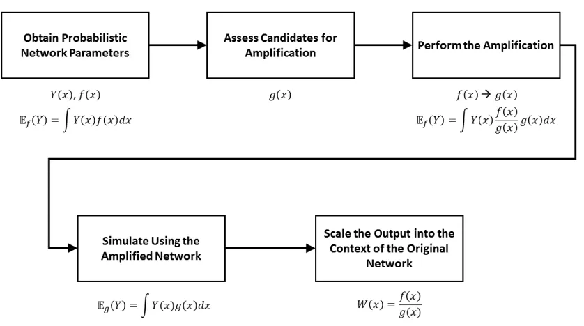
methodology will evaluate each entry of_Lby fulfilling the following steps:

1. Obtain probabilistic network parameters;

2. Assess candidates for amplification;

3. Perform the amplification;

4. Simulate using the amplified network; and

(28)

[image:28.612.101.520.88.322.2]

Figure 4.1: IS Methodology Flowchart

4.3

Importance Sampling Methods

4.3.1 General Method

The generalized IS methodology, seen in Figure 4.1, starts with some metric of interest

Y with possible outcomesY(x). Each outcome, x, occurs with probability f(x). Under

standard simulation, one can calculate the expected value of Y at densityf, represented

by _Ef(Y)[18]. Equation (4.2) shows how to calculate the expected value for a metric of

interest under normal circumstances,

Ef(Y) = Z

Y(x)f(x)dx. (4.2)

Parameters of the network will then be assessed for amplification, whose modification

modifies density f. The changes of measure produce probability densityg for metric Y.

Therefore, each outcome Y(x) would occur at probability g(x) when simulating under

(29)

by g_g is the same as multiplying by one:

Ef(Y) = Z

Y(x)f(x)

g(x)g(x)dx. (4.3)

Pulling away the termf_g from Equation (4.3) gives us the condition by which one would

simulate under amplified conditions:

Eg(Y) = Z

Y(x)g(x)dx. (4.4)

The ratio of density f to density g, given by W can then be utilized to translate the

output of the amplified simulation back to the context of the original network,

W(x) = f(x)

g(x). (4.5)

This translation works by multiplying each outcomeY(x)by each W(x). Ultimately,

the translation works by using W to replace the impact of g with f in the final output

[18]. Scaling the output from the simulation under amplified conditions produces the same

expected value as in equation (4.2):

Eg(Y W) = Z

Y(x)f(x)

g(x)g(x)dx=Ef(Y). (4.6)

4.3.2 Security Framework

The generalized IS methodology is tailored to represent cases where an attacker moves

through a network. The following shows the different variables and sets that will be utilized

in calculating the likelihood of reaching a particular target machine.

SETS:

M: set of all machines.

Z: set of all target machines,Z ⊆M.

(30)

Mv

m(j): set of vulnerable machines accessible from machinemduring attemptj,

M_mv(j)⊆Mm.

Amn: set of services on machinenvisible from machinem.

VARIABLES:

umn(j): probability of targeting machinenfrom machinemon attemptj.

vkmn: probability of targeting servicekon machinenfrom machinem.

q(j): machine/service selection probability during attemptj.

p(j): success/failure probability during attemptj.

x=     

1 If servicekis compromised during attemptj.

0 Otherwise.

τz: compromising time of machinez.

fz(τz): probability that a attacker has reached machinezat compromising timeτz.

gz(τz): probability under amplified conditions.

The attacker operates by leveraging assault attempts against services present on the

machines in the network. Within the total time horizon, T, there is a maximum of J

possible attempts that the attacker can execute. Note that each attempt consumes one unit of

time. During a particular replication, there areΨtrials. Should a target,z, be compromised

during a particular trial ψ ∈ Ψ, the associated indicator variable will take a value of 1.

Otherwise, it will take a value of and0, such that,

Izψ =   

 

1 If targetzis compromised during trialψwithin time horizonT

0 Otherwise.

(4.7)

When utilizing standard Monte Carlo simulation, the likelihood, Lz, that a particular

targetz is compromised is given by the expected value of the indicator variable [4]. It is

(31)

Lz =Ef(Iz) = 1 Ψ Ψ X ψ=1

Izψ. (4.8)

The calculations for the likelihood of reaching a target machine are held with respect

to each trial ψ. Said likelihood is dependent on the targeting, successes, and failures an

attacker experiences while moving through the network. Targeting always is done in two

phases when the attacker seeks to make an assault attempt. The first phase entails the

se-lection of a target machine. From a source, the attacker will look at all accessible machines

that are currently vulnerable. Each individual machine may have a unique selection

prob-ability, but for the purposes of this thesis, every machine is given an equal likelihood of

selection,

umn(j) = 1 |Mv

m(j)|

∀ n ∈M_mv(j). (4.9)

Once a machine has been selected, the attacker will select a vulnerable service on the

targeted machine. Each service is give a weight, which corresponds with an attacker’s

inter-ests and capabilities from a given source machine. The probability of selecting a particular

service is calculated by dividing the service’s weight by the aggregate of all weights on the

machine,

vkmn =

wk P

i∈Amnwi

∀ k ∈Amn, m∈M, n∈Mm (4.10)

The combined actions of selecting a machine and service represents the attacker’s

choice of targeting. Thus, the product of the two selection probabilities represents the

probability of a particular choice during an assault attempt, given by

q(j) =vkmnumn(j) ∀ j ∈ {1,2, ..., J}. (4.11)

(32)

each attempt, the attacker will either have a success or failure. The probability that an

at-tacker succeeds or fails during an assault attempt is dependent on the probability of success

defined for a particular service,

p(j) = px_k(1−pk)1−x ∀ j ∈ {1,2, ..., J}. (4.12)

If given a sufficiently long time period, an attacker would be able to reach every

tar-get. However, the simulation has an established time horizon, T. Therefore, there will

be cases where τz is unknown for a particular machine. The number of attempts required

to compromise a machine of interest is utilized in calculating the likelihood said machine

is compromised. As such, when τz is unavailable,T is used as a substitute, which

corre-sponds withJ attempts. Thus, the number of attempts required to compromise a machine

of interest is shown by

Jz(τz) = min (Number of attempts needed to reachzat timeτz, J). (4.13)

Formally, each assault path to a target has an associated probability. Each attempt

consists of a machine/service selection as well as a success/failure. The product of these

two elements gives each attempt an associated probability value. The combination of all

attempts forms the attacker’s assault path. Thus, the product of all attempt probabilities

gives the likelihood of compromising a machine of interest,

fz(τz) = Jz(τz)

Y

j=1

p(j)q(j) ∀ z ∈Z. (4.14)

When either elements of the success/failure or choice elements are amplified, the

prob-ability of generating a particular assault path becomes altered. When any consistent

(33)

probability of generating an amplified path is given by,

gz(τz) = Jz(τz)

Y

j=1

p0(j)q0(j) ∀ z ∈Z. (4.15)

The ratio of probability densityf to densityg for each target machine is given by:

Wz =

fz(τz)

gz(τz)

∀ z ∈Z. (4.16)

Said ratio is employed when utilizing IS since the calculation of the likelihood is held

with respect to density g rather than density f. Scaling the simulation under amplified

conditions must make use of each Wz. Thus, a modified version of Equations (4.6) and

(4.8) produces the likelihood calculation for IS:

Lz =Eg(IzWz) = 1 Ψ

Ψ

X

ψ=1

IzψWzψ. (4.17)

Tailoring the probability distribution associated with compromising a machine of

inter-est enables the application of IS. Simulation can be conducted under amplified conditions.

Once output data is received, said output can be scaled back into the context of the original

network by utilizing the ratio of the original probability density to the amplified probability

density. Thus, the likelihood a machine of interest is compromised can be determined.

4.4

Implementation Methods

The rare-event simulation techniques described in Section 4.2 are implemented with

ap-plication to a realistic and complex cyber network topology. The model receives several

inputs that are user-defined. Once these inputs are processed, several outputs will be

re-ceived. Figure 4.2 depicts how the IS methodology can be implemented. The required

(34)

1. Number of trials and replications;

2. Network topology and services;

3. Impact and target data;

4. Default service selection weights;

5. Default service success probabilities;

6. Amplifications to weights and success probabilities; and

7. Attacker movement strategy.

Figure 4.2: Model Implementation Structure

Different types of machine movement strategies can be implemented into the attacker

behavior. Depth-based search is one such method that will be evaluated. As seen in

Algo-rithm 1, the number of attempts (j), attacker’s initial starting position, attacker knowledge, target machines, success counter, and failure counter are initialized prior to movement. The

attacker knowledge describes all machines that have been compromised by the attacker so

(35)

event terminates. If the number of attempts does not exceed the maximum number allowed

(J), the assault will continue. The attacker will then scan the outgoing connections attached to its current source node. If all outgoing connections lead to compromised machines, the

attacker will attempt to change its source node such that at least one outgoing connection

leads to an un-compromised machine. If this is impossible, then the network infiltration

event ends. Once the attacker’s position is not a dead-end, then a target machine is chosen.

After a target machine is chosen, a service on the target machine is selected. Said service

is then attacked. The total number of assault attempts will increment by one regardless of

whether the attack is a success or failure. Should the attack be a success, the attacker’s

current position will be updated to be the targeted machine and the attacker knowledge will

be updated. At this time, the algorithm will check if the compromised machine is one of

the target machines. If it is a target, then the likelihood of reaching it will be calculated.

Should all target machines be compromised, infiltration will terminate and the replication

will end.

Breadth-based movement follows a similar methodology to depth-based movement and

is represented by Algorithm 2. The primary key difference is seen when the algorithm

ini-tializes. Breadth-based movement does not establish a source node. Instead, all currently

compromised machines in the attacker knowledge are treated as a collective source.

Ev-ery un-compromised machine stemming from the outgoing connections of this collective

source is a potential target for the attacker.

This distinction between machine selection strategies is displayed in Figures 4.3 and

4.4. Note that Figure 4.3 shows a source node that is used as a pivot point. Said source

is one of the currently compromised machines. Only outgoing, un-compromised machines

from this single pivot point are considered for potential targeting. By contrast, Figure

4.4 shows how all un-compromised machines connected to all compromised machines are

considered for targeting.

(36)

1: j←1

2: SourceN ode←Internet

3: Knowledge←addKnowledge(Internet)

4: T argetM achines←addT argets()

5: whilej < Jdo

6: M achineOptions←availableConnections(SourceN ode)

7: if isDeadEnd(M achineOptions) then

8: if isN ewSourceAvailable(Knowledge) then 9: SourceN ode←chooseN ewSource(Knowledge)

10: M achineOptions←scanConnections(SourceN ode)

11: else

12: break

13: end if

14: else

15: SelectedM achine←machineSelection(M achineOptions)

16: SelectedService←serviceSelection(SelectedM achine)

17: AttackStatus←attackM achine(SelectedService)

18: j ←j+ 1

19: ifisAttackSuccessf ul(AttackStatus)then

20: SourceN ode←updateSourceN ode(SelectedM achine)

21: Knowledge←Knowledge+addKnowledge(SelectedM achine)

22: if isT arget(SelectedM achine, T argetM achines) then

23: recordLikelihood(SelectedM achine)

24: if isAllT argetsCompromised(Knowledge, T argetM achines) then

25: break

26: end if

27: end if

28: end if

29: end if

30: end while

(37)

1: j←1

2: Knowledge←addKnowledge(Internet) 3: T argetM achines←addT argets()

4: whilej < Jdo

5: M achineOptions←[ ] 6: forM achine∈Knowledgedo

7: M achineOptions←M achineOptions+availableConnections(M achine)

8: end for

9: SelectedM achine←machineSelection(M achineOptions)

10: SelectedService←serviceSelection(SelectedM achine)

11: AttackStatus←attackM achine(SelectedService)

12: j←j+ 1

13: ifisAttackSuccessf ul(AttackStatus)then

14: j ←j+ 1

15: SuccessCounter ←SuccessCounter+ 1

16: Knowledge←Knowledge+addKnowledge(SelectedM achine)

17: if isT arget(SelectedM achine, T argetM achines) then 18: recordLikelihood(SelectedM achine)

19: if isAllT argetsCompromised(Knowledge, T argetM achines) then

20: break 21: end if

22: end if

23: end if 24: end while

(38)

Figure 4.3: Depth-Based Machine Selection Example

(39)

assign an impact rating to each target machine should it become compromised. MITRE

has a generalized risk rating system whose categories are cost, technical performance, and

scheduling [12]. A similar impact-rating heuristic is formed whose categories are

opera-tional, financial, and schedule. These categories are rated from1−5with5being the most

severe rating. The operational category describes the impact of the event on the ability

of the organization to perform core business functions, the financial category assesses the

direct implications on the budget, and the schedule category reflects any adjustments that

need to be made to project timelines.

Table 4.1: Impact Heuristic

Operational Financial Schedule 5

Severe Ability to perform core

business function com-pletely crippled.

Exceptional budget im-pact.

Exceptional scheduling adjustments required.

4

Significant Ability to perform core

business function is sig-nificantly impaired.

Budget significantly ex-ceeds planned amounts.

Major scheduling adjust-ments required.

3

Moderate Ability to perform core

business function is mod-erately impaired.

Budget moderately ex-ceeds planned amounts.

Moderate scheduling ad-justments required.

2

Minor Ability to perform core

business function is slightly impaired.

Budget slightly exceeds planned amounts.

Minor scheduling adjust-ments required.

1

Minimal No impact on ability to

perform core business function.

Budget is not affected. No planning adjustments re-quired.

Schedule is not affected. No planning adjustments required.

Although the probability of successfully exploiting a vulnerable service has been

de-fined, the method by which these probability values are determined has yet to be identified.

Each vulnerable service can be assigned a probability using CVSS version 3 [22]. The

methodology by which these values are assigned combine usage of Table 4.2 and Equation

(4.18).

(40)

Table 4.2: CVSS Categorization Values

Metric Category Lower Value Upper Value

Access Complexity (AC)

High 0.418 0.462

Low 0.7315 0.8085

Access Vector (AV)

Physical 0.19 0.21

Local 0.5225 0.5775

Adjacent Network 0.589 0.651

Network 0.8075 0.8925

Privileges Required (PReq)

None 0.8075 0.8925

Low 0.589 0.651

High 0.2565 0.2835

User Interaction (UI)

None 0.8075 0.8925

Required 0.589 0.651

based on its severity. FIRST classifies a methodology for assigning categories to

vulner-abilities [7]. When looking at AV, if the attacker exploits a vulnerable component via the

network stack, the categorization is either Network or Adjacent. Between these two, the

vulnerability can be exploited from a routed network, the categorization is Network. If

the attacker cannot exploit the vulnerability though the network stack, the categorization is

either Local or Physical. If the attack requires physical access to the target, the

categoriza-tion is Physical. The AC can either be Low or High. It is only High if the attacker cannot

exploit the vulnerability at will. PReq can either be None, Low, or High. If the attacker

does not need to be authorized, PReq is categorized as None. If administrator privileges are

required, PReq is High. UI is fairly straightforward. If the attacker requires another user to

perform an action, UI is Required. Otherwise, UI is None [7]. Each of these subcategories

corresponds to a range of scores, which are derived from Zhanget al.[22]. A uniform

dis-tribution is then used to give each service a single score for each subcategory for eventual

use in determining a probabilistic value. Equation (4.18) is then utilized to calculate the

final probability value for each service [22], given that there areK total services,

(41)

Consider CVE-2009-0658 as a potential vulnerability present on a service. According

to Zhanget al.[22], this vulnerability receives Local for AV, Low for AC, None for PReq,

and Required for UI. Table 4.3 shows a potential probability scoring for this particular

vulnerability.

Table 4.3: CVE-2009-0658 Probability Scoring Example Category Subcategory Score

AV Local 0.532

AC Low 0.772

PReq None 0.874

UI Required 0.601 Total Score: 0.455

Each service also takes a selection weight as an input for the IS model. The method by

which these weight inputs are seen is shown in Table 4.4. These weights are assigned to

each service according to the attacker’s interest. Said interest is controlled by an attacker’s

capabilities and intent. Interest is placed into four categories: low, medium, high, and very

high. Each category is given a high and low value which feeds into a uniform distribution

when assigning weights to services. The potential value of the weights exponentially

in-creases as the interest level inin-creases. Said exponential scaling ensures that a service of

very high interest is much more likely to be selected by an attacker than a service of low

interest.

Table 4.4: Interest Rating

Interest Lower Bound Upper Bound

Very High 6.4 9.9

High 1.6 3.2

Moderate 0.4 0.8

Low 0.1 0.2

The final input of the IS model concerns the network topology and services. An input

topology must include information regarding which machines are present on the network

and how said machines are connected to each other. Additionally, the services present

(42)

machine may or may not be visible from a particular source machine when the attacker

leverages assaults; this type of access information must be specified as an input.

Nonethe-less, once all input information has been received, the IS model can be utilized.

4.5

Experimental Methods

Comparison of the proposed IS methodology can be assessed from two distinct

perspec-tives. The first perspective seeks to contrast the quality of risk estimates between methods.

A(1−α)confidence interval can be produced for a static number of runs per replication,

where α is the probability of Type I error. The risk estimates of each test case should

be roughly the same. However, the bounds of the confidence interval should be different.

Confidence intervals with a smaller halfwidth indicate a more accurate risk estimation.

The second perspective seeks to compare the computation effort required by each

tech-nique to ascertain a quality estimate of the network’s risk. First, some measure of a quality

estimator must be established. In the case of this thesis, a quality estimate of risk is given by

a confidence interval that falls within some percentage of the mean. Thus, additional trials

will be run until each confidence interval converges appropriately. Note that convergence

necessitates checking each confidence interval at certain points within the simulation to

make sure it falls within the aforementioned criteria. Expedient convergence indicates less

expenditure of computation effort. Therefore, the number of trials required for convergence

is utilized as a measure of time. Pure computational time is not utilized as a meaningful

metric since different computers have varying hardware, which can obfuscate the utility of

the IS technique.

To increase the efficiency of the simulation, convergence will only be checked at

cal-culated milestones, represented by a specified number of trials for a particular replication.

The first milestone must be established prior to running the simulation. Should

conver-gence not be reached at a milestone, the number of trials needed to recheck converconver-gence

(43)

CONVERGENCE:

Λz: set of likelihoods of compromising targetz ¯

Lz: average likelihood of compromisingz

sz: likelihood standard deviation for machinez

tα

2,|Λz|−1: t-statistic

θ: likelihood quality threshold (%)

ψc

z: number of trials needed before re-checking convergence for machinez.

The confidence interval for the likelihood must converge to be within someθ%of the

mean. Therefore, one can determine the number of trials needed to obtain a quality

esti-mate. For each machine of interest:

¯

Lz(1 +θ)≥L¯z+tα₂,|Λz|−1

sz p

ψc z

(4.19)

SubtractingL¯z from each side of Equation (4.19) gives:

θL¯z ≥tα₂,|Λz|−1

sz p

ψc z

(4.20)

Equation (4.20) can be rearranged to produce:

p

ψc z =

tα

2,|Λz|−1sz

θL¯z

(4.21)

ψ_zc = _t_α

2,|Λz|−1sz

θL¯z 2

(4.22)

Ultimately, the true number of trials needed before checking convergence will be the

maximum of all ψc

z since the likelihood confidence interval needs to converge for all

ma-chines of interest.

When running experiments from both perspectives, it is possible to give additional value

(44)

interest. However, there may be multiple events of interest on a single network; assessing

each event independently would necessitate more total runs. Instead, the attacker can be

allowed to continue moving through the network, even after reaching a single machine of

interest. Thus, statistics can be collected about all events of interest simultaneously during

(45)

Chapter 5

Experimentation

This section discusses the experimentation performed using the IS model. A network

ex-ample is first established, which will be fed into the model as an input. Next, the remaining

experimentation-specific inputs will be identified. Afterwards, the results obtained by the

IS model are shown and discussed.

5.1

Network Example

One of the primary inputs to the IS model is a network topology and services. Thus,

for the purposes of experimentation, such an example network must be defined. For the

purposes of this investigation, the network presented in Figure 5.1 will be utilized as a base

case. This example network is derived from the Collegiate Penetration Testing Competition

held in 2016 [3]. The main network is composed of four sub networks, which have some

connectivity between each other.

The example represents the network infrastructure of a hypothetical healthcare-oriented

facility. All connections between machines are networked, but only some servers are

public-facing. Subnet 1 contains workstations and other machines common in a doctor’s

office. 4482 primarily deals with electronic medical records (EMR). By contrast, 4483 is

billing-oriented. 33223 deals with information technology related issues. DC01 is the

do-main controller which serves as an authentication barrier when seeking access to the file

(46)

Figure 5.1: Network Example - Base Case

workstations. XRAY-13 is a machine capable of producing x-ray images.

Subnet 2 houses the EMR functionality of the facility. WEB02 is the actual EMR

application server, with its information being stored on the DB02 database. Subnet 3 hosts

a variety of functions. WEB01 is a billing application server, with information stored on

the DB01 database. The OPS & WIKI server hosts the IT Wiki. PR runs a public relations

Twitter bot that publishes protein folding research.

Subnet 4’s primary functionality is the development of the aforementioned protein

fold-ing research. FOLDING represents an application server for the research, with information

stored on STORAGE. CI is a continuous integration server and works in conjunction with

the GIT repository server for code development. TS01 is a terminal services application

server that enables the IT workstation to remote into the other workstations on the

net-work. The BASTION server acts as a barrier between the public Internet and the rest of the

subnet.

(47)

3 to determine the success probabilities. Table 5.1 displays each service that is present

on network alongside their machine locations and CVSS categorization assignments. The

assignments for user interaction and privileges required are not shown in the table. Each

service receives a “None” for user interaction and “High” for privileges required. Table 5.1

also shows the interest categorizations utilized for assigning services selection weights.

One of the final required inputs relevant to the network topology concerns the impact

data. For the purposes of this experiment, the attacker seeks to exfiltrate data stores on the

four database servers: FILES, DB01, DB02, and STORAGE. Impact ratings are assigned

to each database in Table 5.2. The aggregate score of all three categories represents the

impact should the machine become compromised.

Various network reconfigurations are assessed in addition to the base case. The first

reconfiguration alternative can be seen in Figure 5.2. The connection between the public

relations server and protein folding application server is modified to be unidirectional. Data

can now only be sent from FOLDING to PR. This case is known as “Modify Connection.”

The second case is shown in Figure 5.3 and is known as “Move Connection.” The

con-nection from 33223 to BASTION has been moved to exist between 33223 and TS01. the

third case sees the additional of new machine functionality to the network. An additional

BASTION server, shown as BASTION2, is added to Subnet 4, as seen in Figure 5.4. This

experimental case is referred to as “New Machine.” Since the data contained on STORAGE

is significantly important to the organization, an additional layer of authentication security

may be desirable. The last alternative modifies the BASTION server to be private-facing,

shown in Figure 5.5, and is labeled as “Public to Private.”

Given these input parameters, the only remaining inputs are the number of trials and

replications as well as the degrees of amplification utilized for experimentation. Attacker

(48)

Table 5.1: Service CVSS Categorization

Services Locations Interest Access Complexity

Access Vector

Domain Controller DC01 High Low Network

Domain File Share FILES,

STORAGE Very High Low Adjacent

EMR Web Application WEB02 High High Adjacent

FreeBSD 9.1 BASTION Moderate High Network

GitLab GIT Moderate Low Adjacent

Internal IT Wiki OPS & WIKI Low High Adjacent

Jenkins CI CI Low High Adjacent

MySQL DB02,

STORAGE Very High High Adjacent

NodeJS Web Application PR Low High Adjacent

Non-HIPPAA/PCI Compliant

Billing Application WEB01 High High Network

Picture Archive and

Communication System XRAY-13 High High Network

PostgreSQL DB01 Very High High Adjacent

Print Application PRINT Low Low Adjacent

Protein Folding Application FOLDING High High Adjacent

Remote Desktop TS01 Moderate High Adjacent

SSH BASTION High High Network

Telnet STORAGE Low Low Adjacent

Terminal Services TS01 Moderate High Adjacent

Tomcat CI Moderate High Adjacent

Ubuntu 16.04-1

WEB02, DB02, DB01, PR,

CI, GIT, FOLDING, STORAGE

Low High Adjacent

Ubuntu 16.04-2 WEB01,

OPS & WIKI Low High Network

Windows 7 4482, 4483 High Low Network

Windows 8 33223 High Low Network

Windows Server 2003 XRAY-13 Moderate Low Network

Windows Server 2008 R2-1 DC01 Moderate High Adjacent

Windows Server 2008 R2-2 FILES Moderate High Network

(49)

Figure 5.2: Network Example - Modify Connection

(50)

Figure 5.4: Network Example - New Machine

(51)

Table 5.2: Impact Assignments

Impact Score

Machine Operational Financial Schedule

FILES 2 1 3

DB01 4 3 2

DB02 4 4 3

STORAGE 4 5 5

5.2

Experimental Setup

At this time, the specific settings given to the simulation will be identified. Each

experi-mental case will be run with30total replications. When testing computational efficiency,

the maximum number of possible trials will be1×108 _{for both depth and breadth-based}

network movement. When testing for the quality of estimate, depth-based movement will

be run at a static50,000trials. Likewise, breadth-based movement will be run with a static

4×106 trials when determining the quality of the estimate; this number is different

be-cause breadth-based cases require significantly more trials to produce quality estimates. In

all experimental cases,α= 0.05and the maximum number of assault attempts the attacker

can levy is J = 10, which allows for multiple machines of interest to be compromised

during a single infiltration event. Different levels of amplification will be tested for

differ-ent experimdiffer-ental cases. Amplification will be carried forth by multiplying all probabilities

of successfully compromising a service on a machine by a given factor. Note that an

am-plification of one corresponds to no network amam-plification; these cases represent usage of

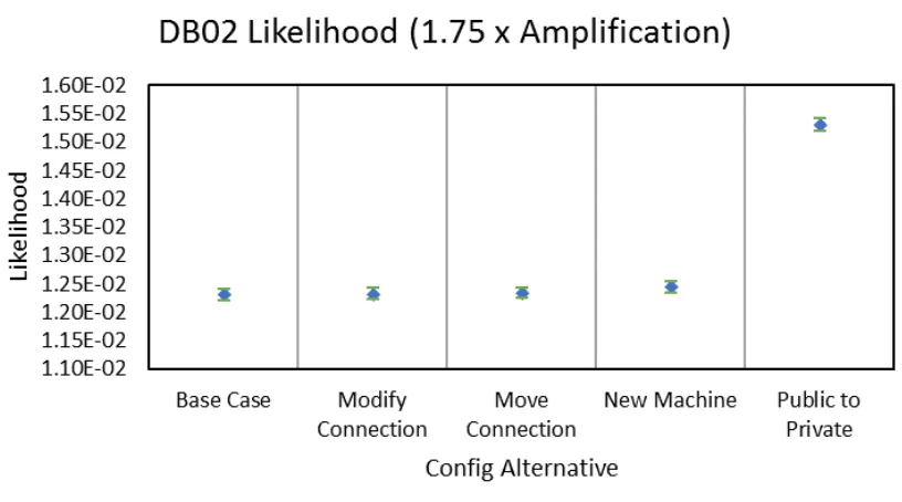
standard simulation as opposed to IS. In total, amplification levels of 1x, 1.25x, 1.5x, 1.75x

and 2x will be tested. Amplification above 2x runs the risk of assigning probability values

(52)

5.3

Base Case Results

5.3.1 Computational Savings - Depth

There is an exponential decrease in the number of trials required to convergence on a quality

likelihood estimation when attackers adhere to depth-based movement. This trend can be

seen in Figure 5.6, which shows that when the degree of amplification shifts from 1x to 2x,

there is about an 83.5% reduction in the computational effort.

Figure 5.6: Convergence - Depth - Base Case - Computational Savings

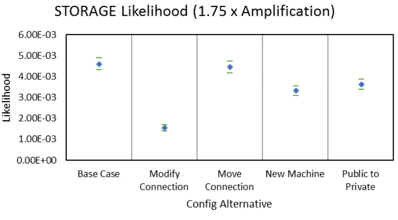
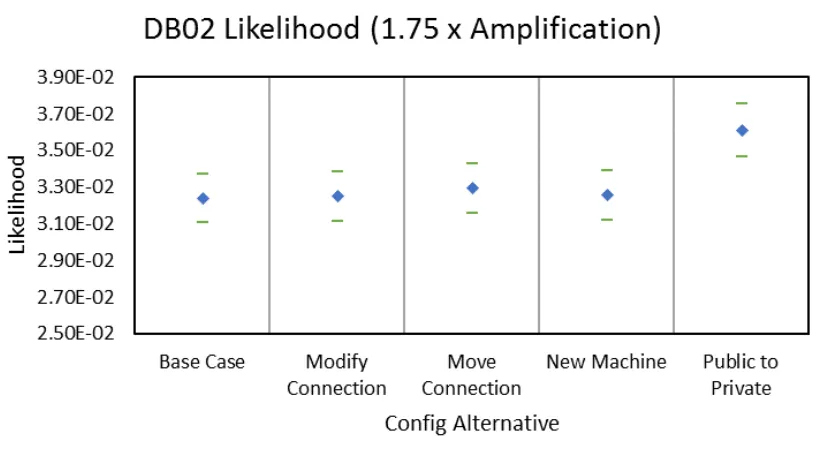
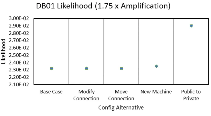
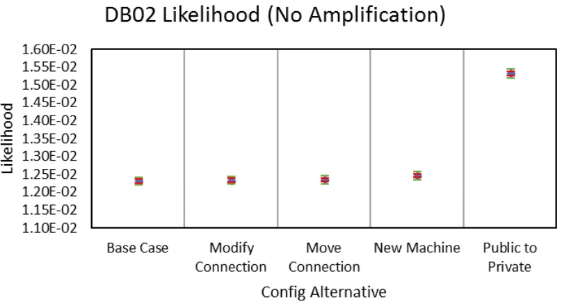
As seen in Figures 5.7 - 5.10, the confidence interval of the likelihood estimates for

compromising all database servers of interest falls within the predetermined±10%of the

mean. The confidence interval for STORAGE remains constant across all degrees of

am-plification. However, for FILES, DB01, and DB02, the confidence interval widens as the

degree of amplification increases. The DB01 and DB02 confidence intervals widen to

nearly touch the±10%limits when approaching 2x amplification.

(53)

Figure 5.7: Convergence - Depth - Base Case - FILES Likelihood

(54)

Figure 5.9: Convergence - Depth - Base Case - DB02 Likelihood

(55)

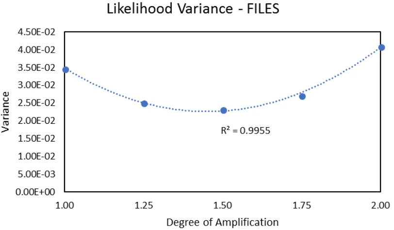
follows a parabolic curve for FILES, DB01, and DB02. For each of these events, the

variance hits a low point at around 1.5x amplification. By contrast, the variance follows an

exponential decrease for STORAGE.

5.3.2 Computational Savings - Breadth

Amplification has a similar effect on computational savings when attackers utilize

breadth-based as opposed to depth-breadth-based movement, as seen in Figure 5.15. As the degree of

am-plification increases, the number of trials required to produce a quality likelihood estimate

exponentially decreases. Shifting the degree of amplification from 1x to 2x decreases the

number of trials by about 79.8%. However, it should be noted that breadth-based movement

required a significantly larger number of trials than depth-based movement.

As seen in Figures 5.16 - 5.19, the confidence interval of the likelihood estimates for

compromising all database servers of interest falls within the predetermined±10%of the

mean. The confidence intervals for FILES, DB01, and DB02 widen as the degree of

ampli-fication increases. However, unlike in Figures 5.7 - 5.10, these confidence intervals are very

far away from the±10%limits. The confidence interval for STORAGE remains relatively

constant across all degrees of amplification although there appears to be a slight sinusoidal

pattern.

The variance of the likelihood estimates for breadth-based movement when running the

convergence method follow similar trends as those seen in Figures 5.11 - 5.14 for

depth-based movement. These figures are shown in Appendix A

5.3.3 Estimate Quality - Depth

Figures 5.20 - 5.23 shows the likelihood confidence intervals for depth-based movement

when running a static number of trials. The confidence interval for STORAGE becomes

tighter as the degree of amplification increase. By contrast, the confidence intervals for

(56)

Figure 5.11: Convergence - Depth - Base Case - FILES Variance

Comparing Cyber Defense Alternatives Using Rare-Event Simulation Techniques to Compute Network Risk

Rochester Institute of Technology

Comparing Cyber Defense Alternatives Using

Thesis Release Permission Form

Acknowledgments

Contents

List of Tables

List of Figures

Chapter 1

Chapter 2

Chapter 3

Network Risk

Risk Reduction

Rare-Event Simulation

Literature Analysis

Chapter 4

Scope of Work

Design Methods

Importance Sampling Methods

VARIABLES:

Implementation Methods

Experimental Methods

CONVERGENCE:

Chapter 5

Network Example

WEB02, DB02, DB01, PR,

FILES 2 1 3

Experimental Setup

Base Case Results