Impulse facility simulation of hypervelocity radiating flows

IMPULSE FACILITY SIMULATION OF HYPERVELOCITY RADIATING FLOWS

R. G. Morgan1_{, T. J. McIntyre}1_{, P. A. Jacobs}1_{, D. R. Buttsworth}2_{, M. N. Macrossan}1_{, R. J. Gollan}1_{, B. R. Capra}1_,

A. M. Brandis1_{, D. Potter}1_{, T. Eichmann}1_{, C. M. Jacobs}1_{, M. McGilvray}1_{, D. van Diem}1_{, and M. P. Scott}1

1_{Centre for Hypersonics, The University of Queensland, Brisbane 4072, Australia}

2_{Faculty of Engineering and Surveying, University of Southern Queensland, Toowoomba, Australia}

ABSTRACT

We describe the X-series impulse facilities at The Univer-sity of Queensland and show that they can produce useful high speed flows of relevance to the study of high temper-ature radiating flow flields characteristic of atmospheric entry. Two modes of operation are discussed: (a) the ex-pansion tube mode which is useful for subscale aerody-namic testing of vehicles and (b) the non-reflected shock tube mode which can be used to emulate the nonequi-librium radiating region immediately following the bow shock of a flight vehicle.

Key words: expansion tube; nonreflected-shock tube.

1. INTRODUCTION

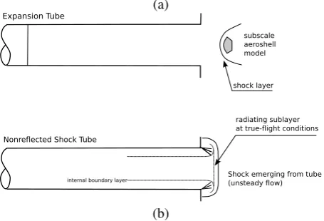
The regions of high speed flight normally associated with significant gaseous radiation are in the upper atmosphere, where the low density makes it difficult to reproduce such flows in ducted facilities, such as shock tubes. Radiating flows can be generated in expansion tubes and may be of sufficient duration to form steady flows around subscale flight vehicle models as shown in Figure 1(a), but experi-ments have to be performed at higher than flight densities and require scaling to interpret the results. As radiant heat transfer does not follow the normal density-length scaling procedures used for wind-tunnel testing, full similarity with the flight conditions is not obtained. In particular, the ratio of convective to radiative heat transfer is differ-ent in flight, as is the coupling of the radiation to the flow field. Typical geometric scale factors range from tens to thousands, indicating that the density levels required for approximate flow similarity in the simulations have to be higher than flight levels by the same sort of factors. Ex-perimental aerodynamic tests of this nature are still worth doing because the techniques for studying radiating hy-personic flows can be developed and validated.

To investigate the fundamental radiation parameters in shock-heated flows, conditions close to real flight den-sities are also required. Experiments could focus on the

(a)

(b)

Figure 1. Layout of the experiments (a) aerodynamic test-ing of a subscale aeroshell, (b) flow behind a bow shock with full physical similarity to flight.

region immediately behind the bow shock of the vehi-cle. This region contains the nonequilibrium radiating zone which is characteristically short, ranging from a few tens of millimetres for small capsules, up to several hun-dred millimetres for upper atmosphere ballute applica-tions. Suitable flow conditions can be achieved in nonre-flected shock tunnels as shown in Figure 1(b), but the low Reynolds numbers lead to rapid boundary layer growth and severely limit the amount of shock-heated test gas that can be generated. Flow slug lengths are typically less than a tube diameter and scale in proportion to the den-sity and the square of the tube diameter. Tunnels suitable for the study of low density, high speed flow therefore require large bores and powerful drivers.

2. THE UQ FACILITIES

The X1, X2 and X3 impulse facilities (Table 1) are free-piston driven expansion tubes which can produce flows at super-orbital speeds, up to 15 km/s [10]. Figure 2 shows the X2 facility as it is used with the driven tube connected directly to the test-section.

Figure 2. The X2 super-orbital impulse facility [11].

configuration will change. For expansion tube opera-tion, the driven tube will consist of a shock tube and an acceleration tube, of equal cross-sectional areas, sep-arated by a light plastic diaphragm. For nonreflected shock tube operation the driven tube will be just a shock tube. In both cases, the free-piston compressor is cou-pled to the upstream-end of the shock tube at the pri-mary diaphragm station. The pripri-mary diaphragm is a heavy, steel diaphragm which regulates the pressures ex-perienced within the tubes during operation.

Table 1. Super-orbital impulse facilities at The University of Queensland.

Facility

X1 X2 X3

overall length (m) 12 20 65

driven-tube bore (mm) 38 85 183

driven-tube length (m) 5 8 36

piston mass (kg) 4 35 470

3. EXPANSION TUBE MODE

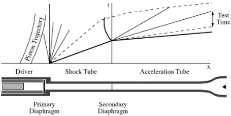
For testing of subscale aeroshell models, the facility is operated in expansion tube mode. The process is shown on the space-time diagram in Figure 3. An example X2 operating condition, relevant to atmospheric entry to Ti-tan, is labelled as shot x2s97 in Table 2.

Although the zero on the time-axis of the space-time dia-gram is at main diaphragm (Figure 3) rupture, the piston has been in motion for approximately 80 ms as it accel-erated along the compression tube and compressed the driver gas. Upon primary-diaphragm rupture, a strong shock is driven through the test gas, raising its pres-sure and temperature and accelerating it up to a speed of 2.7 km/s. This shock reaches the secondary diaphragm which is shattered and left behind in the boundary layer along the acceleration tube. The test gas flowing into the

Figure 3. Schematic diagram of the X2 facility, with noz-zle, operating in expansion tube mode.

acceleration tube expands to final test-flow conditions as it approaches the test-section. The amount of expansion of the test gas is regulated by the initial acceleration-gas pressure and the profile of the nozzle at the downstream-end of the acceleration tube [11].

3.1. Estimation of Operating Conditions

The numerical simulation of the facility is an important part of characterising the free-stream flow that is applied to the aeroshell model. The condition of free-stream flow is estimated from a mix of direct measurements and cal-culations. Operating parameters that can be directly mea-sured are the initial fill pressures and temperatures, the shock speeds, Pitot pressures at the end of the nozzle and static pressures at a number of locations along the driven tube and expansion nozzle. The overall numerical simulation is a combination of a one-dimensional sim-ulation of the high-pressure sections of the facility with an axisymmetric simulation of the low-pressure accelera-tion tube and nozzle. The transient, one-dimensional flow data just upstream of the secondary diaphragn is used as inflow to the subsequent axisymmetric simulation.

The flow through to the end of the shock tube is simulated with the L1d code [4]. Chemical equilibrium (using ther-mochemical data from the CEA program [5]) is usually assumed for this part of the facility because, in regions where the gas temperature is high, the pressure is also high. The one-dimensional nature of the simulation to the downstrean-end of the shock tube is also considered adequate because the boundary layers are relatively thin.

Table 2. Initial (fill) conditions. Gas compositions are given as volume fractions. Initial temperatures are assumed to be room temperature, approximately 23oC.

Shot Identity

x2s97 x3s296 x3s346 x3s347

compressed-air pressure (MPa) 1.75 1.54 1.54 1.54

primary-diaphragm thickness (mm) 1.6 1.6 1.6 1.6

driver-gas composition 0.665 He+0.335 Ar 0.8 He+0.2 Ar 1.0 He 1.0 He

driver-gas pressure (kPa) 48 18.8 18.7 18.7

buffer-gas composition – – 1.0 He 1.0 He

buffer-gas pressure (kPa) – – 3.2 3.2

test-gas composition 0.95 N2+0.05 CH4 0.95 N2+0.05 CH4 air air

test-gas pressure 29 kPa 2.2 kPa 10 Pa 3 Pa

secondary-diaphragm thickness (mm) 0.025 0.025 0.013 0.013

acceleration-gas composition air air – –

acceleration-gas pressure (Pa) 14 5.5 – –

Figure 4. Pressure field in the nozzle during the test pe-riod.

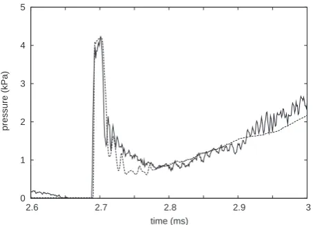
Figure 5 compares the simulated data with the measured pressure from a transducer embedded in the wall near the exit plane of the nozzle. Agreement is good, particularly for the magnitude and duration of the pulse associated with the starting shock structure that is pushed through the nozzle, and then for the subsequent arrival of the un-steady expansion.

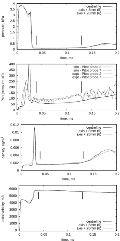
Despite the presence of the shock near the nozzle walls (Figure 4), the core flow conditions, as shown in Fig-ure 6, are reasonably steady and are maintained for a useful length of time of nearly 100 µs. Note that the pressure in the core is approximately 113 Pa, about one tenth of the pressures observed near the nozzle wall. The other estimated flow parameters are M = 18.7, ρ= 1.69×10−3_kg/m3_{,u= 5.72km/s andT = 210K.}

Because the unsteady expansion of the early part of the test gas is rapid, the chemical species tend to be frozen at conditions not far from the high-temperature

composition that existed in the shock tube.

Core-flow mass fractions for this simulation are estimated as N2:0.9452, CH4:3.101×10−5, CH3:8.878×10−8, CH2:2.810×10−9, CH:1.492×10−9, C2:3.441×10−9, H2:5.472×10−3_{, CN:3.274×10}−7_{, NH:6.096×10}−13_, HCN:4.924×10−2_{, N:4.688×10}−17_{, C:1.092×10}−9_,

0 1 2 3 4 5

2.6 2.7 2.8 2.9 3

pressure

(

kPa

)

time (ms)

Figure 5. History of static pressure at the wall, at noz-zle exit. The solid line is measured data while the dashed line is data from the numerical simulation. The zero of the time axis is at secondary-diaphragm rupture. Some low-frequency background noise appears on the measured signal and is particularly noticeable att= 2.6ms.

and H:3.737×10−5. Agreement with the measured Pitot pressure is not particularly good (Figure 6), with the low simulation values being consistent with the shock speed being about 5% lower than that measured in the facility [1]. This was, however, a low resolution simulation and we shall be running future simulations with higher reso-lution grids.

3.2. Radiant Heat Flux Measurement

0 0.5 1 1.5 2 2.5 3 3.5 4

0 0.05 0.1 0.15 0.2

pressure, kPa

time, ms

centreline axis + 8mm (5) axis + 26mm (6)

0 50 100 150 200 250 300 350 400

0 0.05 0.1 0.15 0.2

Pitot pressure, kPa

time, ms

sim - Pitot probe 2 sim - Pitot probe 7 expt - Pitot probe 2 expt - Pitot probe 7

0 0.002 0.004 0.006 0.008 0.01 0.012

0 0.05 0.1 0.15 0.2

density, kg/m

3

time, ms

centreline axis + 8mm (5) axis + 26mm (6)

0 1000 2000 3000 4000 5000 6000

0 0.05 0.1 0.15 0.2

axial velocity, m/s

time, ms

centreline axis + 8mm (5) axis + 26mm (6)

Figure 6. Conditions near the nozzle centerline at the exit plane. The zero of the time axis is aligned with the arrival of the shock and the vertical bars indicate the estimated start and end of the test period.

of pairs of thin-film heat transfer gauges mounted behind quartz windows [2]. Embedded in the aeroshell surface, adjacent to the radiation sensor were two thermocouples which were exposed to the combined radiant and con-vective heat load. Figure 7 shows the response of these sensors for a single shot in the X3 facility. Shots with and without CH4in the test gas showed clearly that sig-nificant radiation occurred only when CH4 was present (Figure 8).

3.3. Optical Imaging

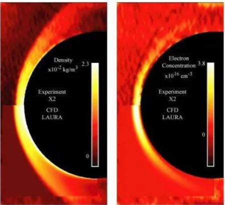
Using the second and third harmonics from a Nd:YAG laser (532 nm & 355 nm), a holographic technique [7] was used to produce interferometric images for the flow of nitrogen around a 15 mm cylinder in a flow with

Figure 7. Total heat flux history for shot x3s294 with the Pathfinder aeroshell model.

Figure 8. Radiative heat flux measurements for the Pathfinder aeroshell model for a number of shots.

free-stream density 0.0014 kg/m3 _{and velocity 10.3 km.} The interferograms were processed using Fourier trans-form and unwrapping techniques to determine the fringe shift at each point and this process gave the distributions shown in Figures 9 and 10 [6]. Agreement with compu-tational data from the LAURA code [8] is good.

4. NONREFLECTED SHOCK TUBE MODE

For emulating the nonequilibrium radiation region fol-lowing a bow shock, the X3 facility is operated in non-reflected shock tube mode with the process shown in Fig-ure 11. Note that the test period is associated with the gas immediately following the primary shock as it enters the test section.

Figure 9. Density and electron concentration around a 15 mm cylinder. The computational data is overlaid on the lower half field of each image.

Figure 10. Density and electron concentration along the stagnation line for a 15 mm cylinder. The shock is located at approximately 1 mm from the body.

medium density gas between the primary and secondary diaphragms is a secondary, shock-heated driver and acts as a buffer between the test gas and the jet of driver gas that is produced during the rupture of the primary di-aphragm. The rupture of the secondary diaphragm is rapid and more uniform across the diameter of the tube

Figure 11. Schematic diagram of the X3 facility operating in nonreflected shock tube mode.

[12].

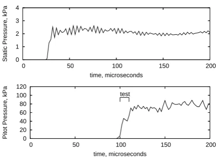
Figures 12 and 13 show the histories of static pressure at a point close to the downstream-end of the driven tube and a Pitot pressure signal from the core flow, a little fur-ther downstream, in the test section. The slow rise of the signals is characteristic at low operating pressures (and is not helped by the low sampling rate that was used for these particular shots). The estimated test period is iden-tified on each of the Pitot pressure signals and the time between the arrival of the primary shock and the subse-quent arrival of the contact surface. At these speeds, we are seeing 200 mm and 100 mm slugs of test gas with the current facility and, with an increase to a 500 mm bore driven tube, we should see substantially longer test slugs [9].

0 2 4 6 8

0 50 100 150 200

Static Pressure, kPa

time, microseconds

0 20 40 60 80 100 120

0 50 100 150 200

Pitot Pressure, kPa

time, microseconds test

Figure 12. Wall static pressure at the end of the driven tube and Pitot pressure history in the test section for shot x3s346.

5. CONCLUDING REMARKS

0 1 2 3 4

0 50 100 150 200

Static Pressure, kPa

time, microseconds

0 20 40 60 80 100 120

0 50 100 150 200

Pitot Pressure, kPa

time, microseconds test

Figure 13. Wall static pressure at the end of the driven tube and Pitot pressure history in the test section for shot x3s347.

bow shock of the flight vehicle can be achieved with the nonreflected shock tube mode of operation. Preliminary experiments and whole-of-tube calculations have been undertaken for a few conditions but further conditions need to be explored and refined calculations need to be made.

ACKNOWLEDGMENTS

This project has been supported, for both development of the expansion tube facilities and of our computational facility, by the Smart State Research Facilities Program of the Queensland State Government, and by the Australian Research Council. Many of the graduate students have been supported by Australian Government Postgraduate Research scholarships.

REFERENCES

1. A. Brandis, R. J. Gollan, M. Scott, R. G. Mor-gan, P. A. Jacobs, and P. Gnoffo. Expansion tube operating conditions for studying non-equilibrium radiation relevant to Titan aerocapture. In 42nd AIAA/ASME/SAE/ASEE Joint Propulsion Conference and Exhibit, AIAA-Paper-2006-4517. American In-stitute of Aeronautics and Astronautics, July 2006.

2. B. R. Capra. Aerothermodynamic simulation of sub-scale models of the FIRE II and Titan Explorer vehi-cles in expansion tubes. PhD Thesis, The University of Queensland, Brisbane, August 2006.

3. P. A. Jacobs. MB CNS: A computer program for the simulation of transient compressible flows; 1998 Up-date. Department of Mechanical Engineering Report 7/98, The University of Queensland, Brisbane, June 1998. http://www.mech.uq.edu.au/cfcfd/.

4. P. A. Jacobs. L1d: a computer program for the sim-ulation of transient-flow facilities. Department of Mechanical Engineering Report 1/99, The University of Queensland, Brisbane, Australia., January 1999. http://www.mech.uq.edu.au/cfcfd/.

5. B. J. McBride and S. Gordon. Computer program for calculation of complex chemical equilibrium compo-sitions and applications II. Users manual and program

description. Reference Publication 1311, NASA,

June 1996.

6. T. J. McIntyre, A. I. Bishop, H. Rubinsztein-Dunlop, and P. A. Gnoffo. Experimental and numerical stud-ies of ionizing flow in a super-orbital expansion tube.

A.I.A.A. Journal, 41(11):2157–2161, 2003.

7. T. J. McIntyre, M. J. Wegener, A. Bishop,

and H. Rubinsztein-Dunlop. Simultaneous

two-wavelength holographic interferometry in a super-orbital expansion tube facility. Applied Optics, 36:8128–8134, 1997.

8. F. McNeil Cheatwood and P. A. Gnoffo. User’s man-ual for the Langley Aerothermodynamic Upwind Re-laxation Algorithm (LAURA). Technical Momoran-dum 4674, NASA Langley Research Center, Hamp-ton, Virginia, April 1996.

9. R. G. Morgan, T. J. McIntyre, R. J. Gollan, P. A. Jacobs, A. Brandis, M. McGilvray, D. van Diem,

P. Gnoffo, M. Pulsonetti, and M. Wright.

Radi-ation measurements in nonreflected shock tunnels. In25th AIAA Aerodynamic Measurement Technology and Ground Testing Conference, AIAA-Paper-2006-2958. American Institute of Aeronautics and Astro-nautics, June 2006.

10. A. J. Neely and R. G. Morgan. The superorbital ex-pansion tube concept, experiment and analysis. The Aeronautical Journal, 98(973):97–105, 1994.

11. M. P. Scott, P. A. Jacobs, and R. G. Morgan. Nozzle development for an expansion tunnel. In Jiang, ed-itor,24th International Symposium on Shock Waves, Beijing, China. Springer, July 2004.