This is a repository copy of Achieving Data Compatibility Over Space and Time: Creating Consistent Geographical Zones.
White Rose Research Online URL for this paper: http://eprints.whiterose.ac.uk/5016/
Monograph:
Norman, P., Rees, P. and Boyle, P. (2001) Achieving Data Compatibility Over Space and Time: Creating Consistent Geographical Zones. Working Paper. School of Geography , University of Leeds.
School of Geography Working Paper 01/06
Reuse
See Attached
Takedown
If you consider content in White Rose Research Online to be in breach of UK law, please notify us by
ACHIEVING DATA COMPATIBILITY OVER SPACE AND TIME: CREATING
CONSISTENT GEOGRAPHICAL ZONES
Paul Norman 1 Philip Rees 1
Paul Boyle 2
1
School of Geography
University of Leeds, Leeds, LS2 9JT, UK
e-mail [email protected]
e-mail [email protected]
2
School of Geography and Geosciences
University of St Andrews, St Andrews, KY16 9ST, UK
e-mail [email protected]
CONTENTS
ABSTRACT iii
LIST OF TABLES iv
LIST OF FIGURES iv
1. INTRODUCTION 1
2. WARD BOUNDARY CHANGE SCENARIOS 3
3. APPROACHES TO CREATING CONSISTENT GEOGRAPHIES 5
3.1 Freeze history 5
3.2 Update to contemporary zones 5
3.3 Construct designer zones 6
3.4 Geocode individual/household-level data 7
3.5 Data availability for establishing a consistent ward geography in Eastern
Region 8
4. GEOGRAPHICAL DATA CONVERSION USING LOOKUP TABLES:
GENERAL PRINCIPLES 11
4.1 Geographical data conversion: background 11
4.2 Lookup table concepts 12
4.3 Defining geographical data conversion lookup table frameworks 13 4.4 Lookup tables for geographical data conversion: worked example 18
4.5 Choice of GCT or GML framework 19
4.6 Deriving intersection weights for imperfect (dis)aggregations 20
5. CREATING A CONSISTENT GEOGRAPHY USING GEOGRAPHICAL
CONVERSION TABLES 21
5.1 Postcode locations for geographical data conversion 21
5.2 ED Building-Brick approach to data conversion 26
5.3 Postcode-Point approach to data conversion 46
7. A CONSISTENT GEOGRAPHY FOR WELWYN-HATFIELD: WORKED
EXAMPLE 56
8. CONCLUSIONS 60
ACKNOWLEDGEMENTS 64
ABSTRACT
Geographers have long-recognised the importance of boundary specification and the
problems of using arbitrarily defined areas for the collection and dissemination of
socioeconomic data. The focus has tended to be on the modifiable areal unit problem
and on custom zone design with the problems created by temporal inconsistencies in
zonal boundaries having less consideration. This is surprising as alongside occasional
major structural reorganisations the UK experiences frequent administrative boundary
changes causing difficulties in producing comparable statistics over time. Unless a
consistent geographical approach with time-series data is taken it cannot be known
whether changes are real or an artefact of boundary changes.
The late 1990s has seen initiatives from ONS to promote harmonisation of
geographical information and the Update UK Area Masterfiles (UUKAM) project
which allows the conversion of data between 1991 census and various late-1990s
geographies. For studies which predate the ONS initiative and exceed the data
conversions possible through the UUKAM project, a method must be devised to
establish a data time-series on a consistent geographical basis otherwise the data
quality will be compromised and analyses cannot objectively be compared over time.
After illustrating the nature of the boundary change problems to be overcome, this
paper describes and appraises methods by which data can be adjusted to an
appropriate geography. The paper concludes with a list of advised checks for
researchers carrying out similar work.
LIST OF TABLES
1. Joining boundary and population tables using a common geographical
reference 11
2a. GCT data conversion from ‘many’ source zones to ‘many’ target zones 18
2b. GML data conversion from ‘many’ source zones to ‘many’ target zones 18
3. Availability of relevant lookup table information 26
4. Postcode-ward-ED linked lookup table variables 32
5. Ward numbers in the 1989-98 ward pedigree 34
6. Ward of year-postcode-ward 1998 linked lookup table variables 49
LIST OF FIGURES
1. Ward boundaries 1991 and 1998, Welwyn-Hatfield district 4
2. Types of links between sets of geographical zones 14
3. One to many relationships (disaggregation) 15
4. Many to one relationships (aggregation) 16
5. Many to many relationships (disaggregation-reaggregation) 17
6. 1991 postcode point and ED population distributions in Eastern Region 23
7. Constituent postcodes of wards in 1991 and 1998 (Haldens/Panshanger) 24
8. ED Building-Brick data disaggregation-reaggregation approach 27
9. Algorithm to calculate ‘freeze history’ source-target GCT1 weights 35
10. Algorithm to calculate ‘update to contemporary zones’ source-target GCT2
weights 36
11. Algorithm to use GCTs to carry out data disaggregation-reaggregation process
36
12. Adjustment of hypothetical populations to 1998 geography, ED version 1 38
13. Proportional change of ward populations 1997-98 38
14. Adjustment of hypothetical populations to 1998 geography, ED version 2 40
15. Ward boundaries 1991 and 1998, Thurrock and Peterborough Unitary
Authorities 41
16. Estimated and original ED and ward populations 42
17. Estimated and original ED and ward populations 44
18. Postcode and household counts for each ED 45
20. Algorithm to calculate ward of year-postcode-ward 1998 GCT weights and
adjust input data to target geography 50
21. Adjustment of hypothetical populations to 1998 geography, Postcode-Point
household count approach 51
22. Adjustment of hypothetical populations to 1998 geography, Postcode-Point
postcode count approach 52
23. Percentage differences between the use of household and postcode counts 52
24. Relationships between ward-level postcode and household counts with
population 54
25. Comparison of postcode point and UUKAM estimated SAS populations 55
26. Crude death rates in Welwyn-Hatfield using non-consistent geographical
boundaries 58
27. Crude death rates in Welwyn-Hatfield using consistent geographical
ACHIEVING DATA COMPATIBILITY OVER SPACE AND TIME: CREATING
CONSISTENT GEOGRAPHICAL ZONES
1. INTRODUCTION
Geographers have long-recognised the importance of boundary specification and since
the development of high-performance computing and Geographical Information
Systems (GIS) much progress has been made in addressing problems posed by the use
of arbitrarily defined areas for the collection and dissemination of socioeconomic data
(Blake et al. 2000). Observations that different statistical results are obtained when
different geographical boundaries and area subdivisions are used (Openshaw 1991)
has led to a focus on the modifiable areal unit problem (MAUP) (Openshaw and
Taylor 1981) and on custom zone design (Openshaw and Rao 1995). However, the
problems created by temporal inconsistencies in zonal boundaries have had less
consideration.
Alongside occasional major structural reorganisations the UK is subject to more
administrative boundary changes over time than the rest of Europe put together (ONS
2000). For example, ward boundaries are regularly adjusted in response to population
change to ensure that each local authority has similar councillor/elector ratios
(UKSGB 2000) and the local government structure of the UK was substantially
revised in the late 1990s with the creation of new unitary authorities in some areas
(Wilson and Rees 1999). Furthermore, even if boundaries do not change, area names
and reference codes often vary with different versions and spellings used across years
and between different data suppliers. These issues are compounded by the large
This degree of change and complexity causes difficulties in the production of
comparable statistics over time. Unless a consistent geographical approach with
time-series data is taken it cannot be known whether changes are real or an artefact of a
boundary change. The broader context of this research is to estimate ward-level
populations and calculate Standardised Mortality Rates (SMRs) for each mid-year
1990-1998 for the National Health Service (NHS) Eastern Region Public Health
Observatory (ERPHO). However, the ward boundaries in Eastern Region have been
potentially undergoing both small incremental changes throughout the 1990s as well
as more substantial changes in the number and names of the wards with local
government restructuring. In the former case, incremental changes are very difficult to
determine, in the latter, the fact that structural changes have occurred is readily
identifiable but details about the boundary changes are not.
ONS (2000) recognise it is critical to adopt a coordinated approach to geography and
a need to be consistent in the use of names, codes and references. As a result,
mechanisms are now in place to promote harmonisation within National Statistics
including the ONS Geographic Referencing Strategy and the establishment of
Gridlink, a core set of postcode location data. Addressing some of these issues, the
Updated UK Area Masterfiles (UUKAM) project allows the conversion of data
between 1991 census and various late-1990s postal and administrative geographies
(Simpson 2001).
Since the study period predates the ONS initiative and exceeds the data conversions
time-series on a consistent geographical basis otherwise the data quality will be
compromised and the population estimates and SMRs cannot objectively be compared
over time. After an illustration of the nature of the boundary change problems that
need to be overcome, this paper describes and appraises methods by which data can
be adjusted to the most appropriate geography for the application. An example of data
presented in both non-consistent and consistent geographical bases is given and the
paper concludes with a list of advised checks that researchers should carry out if
attempting similar work.
2. WARD BOUNDARY CHANGE SCENARIOS
To carry out research over time at the electoral ward scale, three boundary change
scenarios may need to be overcome. These are described below and illustrated in
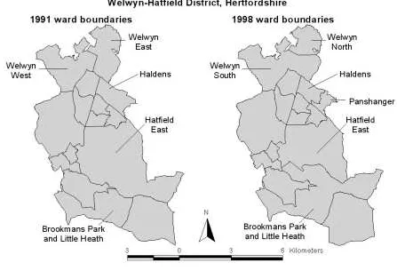
Figure 1 which shows the 1991 Census wards and 1998 electoral wards for
Welwyn-Hatfield, a local authority district in Hertfordshire.
1. In the north of the district, the 1991 wards Welwyn West and Welwyn East
have changed to Welwyn South and Welwyn North by 1998. The new wards
occupy the same combined area as previously but the boundary between the
two has changed.
2. To the south of these in 1991 is Haldens ward which by 1998 had been
subdivided with the creation of an additional ward, Panshanger.
3. In the central and southern parts of the district in 1991 are the wards of
Hatfield East and Brookmans Park and Little Heath. The 1998 boundaries
show that a substantial part of Hatfield East has been transferred to
It is straightforward to identify that wards have changed name (and/or reference code)
and that new wards have been created. However, when ward names stay the same but
their areal extents alter this is impossible to identify without detailed maps. Moreover,
without a time-series of digital boundaries or regular surveillance of Hansard it is
difficult to know when boundary changes take place. In fact the alterations to the
wards in Welwyn-Hatfield were in May 1991 (Baker 1991) just after the Census
thereby creating difficulties in the interpretation of data relevant to the post-Census
[image:10.595.89.536.341.646.2]geography.
Figure 1: Ward boundaries 1991 and 1998, Welwyn-Hatfield district
3. APPROACHES TO CREATING CONSISTENT GEOGRAPHIES
Various strategies can be taken to standardise spatial systems to address the problem
of establishing time-series data on a consistent geographical basis when zone
boundaries change over time. These strategies include ‘freezing geographical history’,
‘updating to contemporary zones’, ‘constructing designer zones’ and ‘geocoding
individual/household data’.
3.1 Freeze history
The freeze history approach involves fixing the zone system at a point in time and
systematically tracking boundary changes so that later observations can be adjusted
back to the original boundaries. This approach is adopted by EUROSTAT for
monitoring trends at the most detailed NUTS5 regional level (Blake et al. 2000). It is
also possible to use areal interpolation, a technique that involves the apportionment of
data from one set of zones to another. In its simplest form the size of the source and
target zones is used to weight the source zone values by the area of overlap with the
target zone (Flowerdew and Green 1994). This is the method used by White et al.
(1998) to fit data from other time periods to 1911 Registration Districts for the
analysis of long-term change. A disadvantage of freezing geographical history is that,
over time, the chosen zones will become less appropriate to current applications.
3.2 Update to contemporary zones
An alternative approach is to update data from previous spatial systems to a set of
contemporary zones. This is also achievable by areal interpolation but can involve the
use of lookup tables (LUTs) to link building-bricks from a previous geography to the
current system thereby enabling the conversion of earlier data (Wilson and Rees 1998,
amendments and can supply LUTs of changes in ED/ward relationships. This
approach is applicable for ward geographies but needs continual attention to note the
boundary changes. A difficulty of using LUTs for data conversion is that direct
measures of the weights to be applied to convert from one geography to another are
rarely available so that surrogate measures must be used. In the ONS LUTs data
conversion weights can be derived since the number of persons involved in the
boundary change is noted. For other applications weights can usefully be derived
using postcode/household counts from a source such as the UK Enumeration District
(ED) to postcode directories. Since postcode locations can be used as small
geographical data conversion building-bricks flexibility in subsequent aggregation is
possible. Penhale et al. (2000) use GIS intersections of 1991 EDs and 1998 wards
with postcode counts of delivery points as a proxy for population distribution to
apportion data where EDs are split.
3.3 Construct designer zones
Another solution is to construct designer zones from smaller building-bricks to
harmonise the zonal system based on boundaries that are common in different years.
This approach is complex to apply and the harmonised boundary solutions may not
match current geography. Moreover, to carry out research on relatively large study
regions the necessary GIS digital boundary sets must be available for all time periods
and even when they are there can be no guarantee that digitising discrepancies
(through either error or changes in areal definitions) do not suggest boundary changes
when none have occurred. For an analysis of inter-regional migration in Australia,
Blake et al. (2000) attempted the assembly of small building-bricks to generate
designer zones with coincident outer boundaries across a number of censuses.
automated solution, so successive overlays of boundaries had to be checked manually
followed by estimation of the area and size of population involved and a search for the
nearest consistent boundary. Apart from being laborious, this approach became a
compromise between the competing goals of temporal consistency and the
maintenance of the functional integrity of the statistical division zones.
A further designer zone approach includes the creation of a new set of areas to
represent the data in a more realistic way than existing administrative geographies
(Openshaw and Rao 1995), though what may be deemed realistic at one time may be
inappropriate at another. Developing an earlier approach by Norris and Mounsey
(1983), Bracken and Martin’s (1995) surface models of 1981 and 1991 census data
enable moves from conventional geographies with the raster cell values used as
building-bricks to be aggregated into user-defined zones. Despite this utility it is only
during a census year when detailed and nationally consistent small area
sociodemographic data become available that a UK population surface can be
generated. Moreover, the complexity of linking data precludes their use as a means of
establishing a standard geography for a year by year data time series.
3.4 Geocode individual/household-level data
The geocoding of individual/household-level data to discrete addresses avoids the
difficulties noted above. Data can be assembled for the most appropriate set of
boundaries to the problem being investigated ensuring temporal consistency and
application relevance. The main constraints relate to cost of establishment and the
need in many applications to guarantee confidentiality. This approach is being
3.5 Data availability for establishing a consistent ward geography in Eastern Region
In practice, the choice of method is largely dictated by the nature, availability and cost
of the input data rather than necessarily being application-driven. In the research
being reported here datasets will only be used that are nationally consistent, widely
available and inexpensive to academics, government organisations, health authorities
and other health professionals. Given a need for a recent geography the aim is to
standardise the ward input data needed for 1990-98 annual population estimates and
SMRs to the 1998 ward geography, the latest year for which all input data are readily
available. The ward-level data sets to be adjusted comprise i) 1991 Census
populations and migrant counts ii) the electorate for each year 1990-98 and iii) the
Vital Statistics births and deaths data for each year 1989-98. The most straightforward
approach by which the ward data could be updated to the 1998 ward geography would
be to intersect polygon GIS coverages for each year with 1998 and, assuming equal
population density, to adjust the inputs based on area of overlap using simple areal
interpolation. Unfortunately, the only appropriate GIS coverages freely available are
1991 ward and Enumeration District (ED) boundaries and the 1998 Unitary Authority
boundaries so that GIS intersection approaches are impossible. (N.B. 1998 ward
boundaries are available to this project through a special arrangement with OS, see
Acknowledgements section g, but will only be used for illustrative purposes and not
for GIS geometrical techniques.) The designer zone approach referred to above is
unnecessary since it is a ward geography that is required. This is not to say that
electoral wards are necessarily the ‘correct’ geography for health applications since
convenient and frequently-used administrative geography of relatively small size for
which sociodemographic data are regularly collected and disseminated.
Household-level geocoded data are outside the data-acquisition scope of this research
but the potential still exists to create a consistent frozen geography if data are
available for units that are small enough to be able to construct zones at one point in
time from those at another. Shaw et al. (1998) point out this is feasible in post-1981
mortality studies since the postcode of last residence is attached to computerised files.
In the UK there are about 1.7 million postcodes covering approximately 25 million
addresses. Postcodes are created and maintained by Royal Mail to enable the efficient
delivery of mail (Raper et al. 1992). The postcode has evolved since the early 1960s
as key data to provide a spatial reference (UKSGB 2001) with the utility of the
postcode system as a geographical referencing system acknowledged in the Chorley
Report on the Handling of Geographic Information (DoE 1987). Pertinently the report
notes that data are collected for numerous incompatible geographical regions which
do not nest into each other and do not have boundaries consistent over time. Heywood
(1997) notes some drawbacks of the postcode as a spatial reference but believes
Chorley’s endorsement of the unit postcode changed the way most socioeconomic
data are managed with their widespread adoption for spatial referencing by many
types of organisations (Raper et al. 1992). In 1991 postcodes were recorded for the
first time on individual census forms and provided the basis for the creation of the
Postcode-Enumeration District Directory (PCED) by the then Office of Population
Censuses and Surveys (OPCS). Postcode locations allow detailed data modelling
small size at unit level (typically 14 residential addresses) which offers versatility for
aggregation into other areal units (Martin 1992).
The UUKAM project (Simpson 2001) demonstrates data conversion using LUTs to
link 1991 geographies to 1998 zones using postcode counts to derive apportionment
weights between the geographies but links from other years are not available. Various
postcode-based LUTs are available to the academic community via Manchester
Information and Associated Services (MIMAS) that enable linkage between
geographical areas and between time periods (MIMAS 1999). Before reporting the
detailed method by which ward-based data for all the years in the study period can be
adjusted to be consistent with the 1998 ward geography, it is useful to examine the
4. GEOGRAPHICAL DATA CONVERSION USING LOOKUP TABLES:
GENERAL PRINCIPLES
4.1 Geographical data conversion: background
Lookup tables (LUTs) are database devices whereby sets of entities in different files
can be linked using reference items that are common between each file. In GIS
packages this type of database operation is carried out when tables of ward-based
population data are ‘joined’ to an attribute table of vector ward boundaries using an
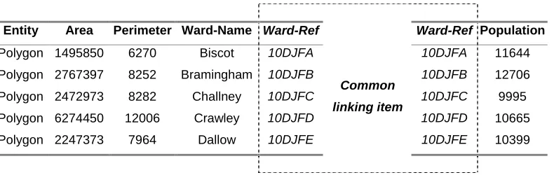
[image:17.595.94.489.327.452.2]item, in this case the ward reference code, that is present in both tables (see Table 1).
Table 1: Joining boundary and population tables using a common geographical
reference
Entity Area Perimeter Ward-Name Ward-Ref Ward-Ref Population
Polygon 1495850 6270 Biscot 10DJFA 10DJFA 11644
Polygon 2767397 8252 Bramingham 10DJFB 10DJFB 12706
Polygon 2472973 8282 Challney 10DJFC 10DJFC 9995
Polygon 6274450 12006 Crawley 10DJFD 10DJFD 10665
Polygon 2247373 7964 Dallow 10DJFE
Common
linking item
10DJFE 10399
A frequent problem in many applications is that the areal units for which data are
available are not necessarily the units that are required (Flowerdew and Green 1994).
A specialised subset of database LUT operations is their use for the conversion of data
from one geographical zonal system to another with the LUT entities being sets of
discrete geographical spatial units. The main purposes of geographical data
conversion LUTs are to enable (Simpson 2001):
• The transformation of 1991 Census data from standard output (Enumeration
Districts, wards, districts, etc.) to: recent postal geography; revised local
government or electoral areas; special planning areas (enterprise zones, national
• The aggregation of data to units sufficiently large to provide reliable results (e.g.
from postcoded events to local authority district).
• Analysing and presenting results for areas familiar to the audience of the research
(e.g. new health areas such as Primary Care Groups).
• Merging of data sets drawn from different sources (e.g. for neighbourhood profiles
containing both census and postal geography data).
• Estimating a time-series on a consistent geographical basis (e.g. Vital Statistics
from wards before and after boundary changes).
4.2 Lookup table concepts
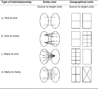
Various types of database links can exist between LUT entities. Wilson and Rees
(1998) conceptualise the relationships between sets of zones that are relevant to the
handling of geographical data. Figure 2a illustrates simple ‘one to one’ links which, in
terms of geographical zonal systems, occurs when zone names change, but boundaries
do not. ‘One to many’ relationships are shown in Figure 2b whereby a source area
may be disaggregated into a subset of smaller target areas, for example, the situation
existing between Census wards and their constituent Enumeration Districts (EDs).
The reverse situation illustrated by Figure 2c shows ‘many to one’ links whereby the
source geography perfectly aggregates into a larger target geography. Essentially a
nested geographical hierarchy, this circumstance often exists at a single point in time
(e.g. Census EDs aggregate to wards which aggregate to local authority districts etc.;
unit postcodes aggregate to postal sectors which aggregate to postal districts etc.) but
boundaries are not necessarily consistent between time points. The ‘many to many’
relationships shown by Figure 2d exist when a zone in the source geography intersects
with several zones in the target geography and similarly a zone in the target
lack of coterminous boundaries between census and postal geographies (Martin 1996).
The data conversion necessary in this situation is a disaggregation of the source
geography followed by a reaggregation into the target geography.
4.3 Defining geographical data conversion lookup table frameworks
The first three relationships described above may be readily defined for standard
geographical zonal systems but ‘many to many’ links and non-standard aggregations
and disaggregations require LUTs to be devised for data conversion from source to
target geographies. The fundamental information necessary within data conversion
LUTs are reference codes to both the source geography in which the data pre-exist
and the target geography into which the data are to be converted together with an
indication of the extent of overlap, a weight, between each zone in the source
geography and each zone in the target geography. These weights, taking a value of
more than zero but less than or equal to one, will sum to one across intersections by
source area (Simpson 2001; Wilson and Rees 1998). Weights are not needed if the
link is a one to one change of name relationship or if the links are one to many or
many to one calculated on a simple ‘best-fit’ basis; the latter being a list of source
zones paired up with the target zone in which the majority of the source zone lies.
Whilst crude, this is often used if information needed to apportion source to target
Figure 2: Types of links between sets of geographical zones
Type of link/relationship Entity sets Geographical units
Source to target units Source to target units
a. One to one
b. One to many
c. Many to one
d. Many to many
Source: after Wilson and Rees, 1998: 2
To support what is essentially a ‘building-brick’ approach, the information in data
conversion LUTs can be organised in two different frameworks both of which have
the ability to support the relationships illustrated in Figure 2. The first LUT
framework is a ‘Geographical Conversion Table’ (GCT) and the second a
‘Geographical Membership List’ (GML). These frameworks are described and
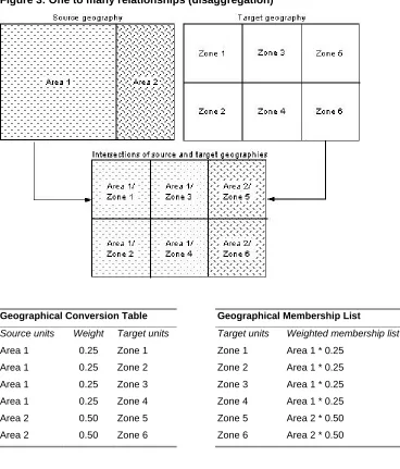
Figure 3: One to many relationships (disaggregation)
Geographical Conversion Table Geographical Membership List
Source units Weight Target units Target units Weighted membership list
Area 1 0.25 Zone 1 Zone 1 Area 1 * 0.25
Area 1 0.25 Zone 2 Zone 2 Area 1 * 0.25
Area 1 0.25 Zone 3 Zone 3 Area 1 * 0.25
Area 1 0.25 Zone 4 Zone 4 Area 1 * 0.25
Area 2 0.50 Zone 5 Zone 5 Area 2 * 0.50
Area 2 0.50 Zone 6 Zone 6 Area 2 * 0.50
Diagrammatic maps of source and target geographies and their intersections in Figure
3 illustrate the one to many relationships conceptualised in Figure 2b showing how
Area 1 of the source geography is disaggregated into Zones 1 to 4 of the target
geography and Area 2 is disaggregated into Zones 5 and 6. Each line of the GCT
framework has a reference to a source unit, the target unit that the source unit is
associated with and a weight to indicate the amount of overlap between source and
target units; the first line showing that 0.25 of Area 1 overlaps with Zone 1. In the
GMT framework the same data is arranged differently so that each line has a
building-brick source unit. The weights indicate the proportion of the source units
[image:22.595.85.480.145.553.2]used for the building-brick.
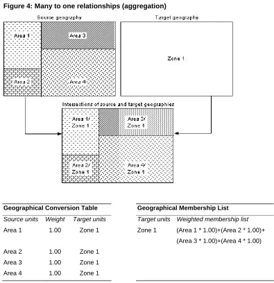
Figure 4: Many to one relationships (aggregation)
Geographical Conversion Table Geographical Membership List
Source units Weight Target units Target units Weighted membership list
Area 1 1.00 Zone 1 Zone 1 (Area 1 * 1.00)+(Area 2 * 1.00)+
(Area 3 * 1.00)+(Area 4 * 1.00)
Area 2 1.00 Zone 1
Area 3 1.00 Zone 1
Area 4 1.00 Zone 1
Figure 4 illustrates the many to one relationships shown in Figure 1c that are the
reverse of the previous situation. The maps show that Areas 1 to 4 of the source
geography wholly nest into Zone 1 of the target geography. Thus the GCT shows the
link between each source unit and associated target unit each with a weight of 1.00
since all of every source unit overlaps the target. The GML arrangement of the data
Figure 5: Many to many relationships (disaggregation-reaggregation)
Geographical Conversion Table Geographical Membership List
Source units Weight Target units Target units Weighted membership list
Area 1 0.25 Zone 1 Zone 1 (Area 1 * 0.25)+(Area 2 * 0.50)
Area 1 0.25 Zone 2 Zone 2 (Area 1 * 0.25)+(Area 2 * 0.50)
Area 1 0.25 Zone 3 Zone 3 (Area 1 * 0.25)+(Area 3 * 0.25)
Area 1 0.25 Zone 4 Zone 4 (Area 1 * 0.25)+(Area 3 * 0.75)
Area 2 0.50 Zone 1
Area 2 0.50 Zone 2
Area 3 0.25 Zone 3
Area 3 0.75 Zone 4
The more complex many to many relationships previously shown in Figure 1d are
illustrated in Figure 5. The diagrammatic maps show that each source unit contributes
to more than one target unit and that each target unit receives contributions from more
than one source unit. The GCT defines the weight by which the source unit should be
disaggregated to its associated target zone with the first line showing that 0.25 of Area
1 overlaps with Zone 1. The GML shows a weighted list of the building-bricks of
each target unit. For example, Zone 1 of the target geography consists of 0.25 of Area
Table 2a: GCT data conversion from ‘many’ source zones to ‘many’ target zones
1. Source unit populations
2. Geographical Conversion Table
3. Estimates for intersections
4. Estimates for target units Source ref. Population Source ref. Weight Target
ref. Disaggregated data Reaggregated data
Area 1 1500 Area 1 0.25 Zone 1 1500*0.25=375 Zone 1 375+500=875
Area 2 1000 Area 1 0.25 Zone 2 1500*0.25=375 Zone 2 375+500=875
Area 3 400 Area 1 0.25 Zone 3 1500*0.25=375 Zone 3 375+100=475
Area 1 0.25 Zone 4 1500*0.25=375 Zone 4 375+300=675
Area 2 0.50 Zone 1 1000*0.50=500
Area 2 0.50 Zone 2 1000*0.50=500
Area 3 0.25 Zone 3 400*0.25=100
Area 3 0.75 Zone 4 400*0.75=300
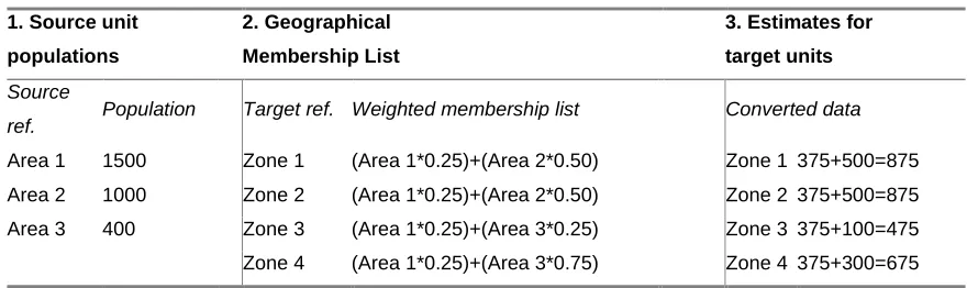
Table 2b: GML data conversion from ‘many’ source zones to ‘many’ target zones
1. Source unit populations
2. Geographical Membership List
3. Estimates for target units
Source
ref. Population Target ref. Weighted membership list Converted data
Area 1 1500 Zone 1 (Area 1*0.25)+(Area 2*0.50) Zone 1 375+500=875
Area 2 1000 Zone 2 (Area 1*0.25)+(Area 2*0.50) Zone 2 375+500=875
Area 3 400 Zone 3 (Area 1*0.25)+(Area 3*0.25) Zone 3 375+100=475
Zone 4 (Area 1*0.25)+(Area 3*0.75) Zone 4 375+300=675
4.4 Lookup tables for geographical data conversion: worked example
To illustrate data conversion when many to many LUT relationships exist, the weights
given in Figure 5 have been applied to hypothetical populations. In Table 2a the
population counts (column 1) are converted from source to target geographies using
the GCT approach. This is achieved by applying the weights in the GCT (column 2)
to the source unit populations to estimate population counts in the source/target
intersections (column 3). These intersection population estimates are then
reaggregated into the relevant target units (column 4). In Table 2b the GML approach
is adopted. The source unit populations (column 1) are apportioned into
bricks using the weights in the GML (column 2). The membership lists of
4.5 Choice of GCT or GML framework
Although the GCT and GML frameworks basically contain the same information
there can be advantages to either approach. In terms of the literature it should be noted
that various data conversion LUT terms exist: a GCT is equivalent to a SASPAC
‘gazetteer’ file (SASPAC 1992: 7/57-7/62) and a GML is equivalent to a SASPAC
‘new zone … using areas’ procedure (SASPAC 1992: 7/63-7/65) and is analogous to
‘area constitutions’ in ONS parlance (ONS 2000). Wilson and Rees (1998: 20)
compare SASPAC ‘gazetteer’ and ‘new zone … using areas’ procedures. For
converting census data an advantage of the latter is that subtractions as well as
additions are feasible so that a target zone can be defined as comprising (Ward01) +
(Ward02 – ED03); thereby avoiding error propagation due to data blurring if just a list
of EDs were used. In this way Wilson and Rees (1998: 46) utilise a GML approach to
define a LUT of 1998 local authority areas in terms of 1991 Census areas that enables
conversion of 1991 Census data into the 1998 geography.
The GCT framework in comparison with the GML approach is more straightforward
to write generic computer programs for and potentially more versatile. This is
exemplified by the UUKAM project (Simpson and Yu 2000; Yu and Simpson 2000;
Simpson 2001) and the use of the All Fields Postcode Directory to convert data
between pairs of administrative, electoral, census and postal geographies. Ultimately,
the choice of GCT or GML framework for converting data from a set of source to
target units will depend on a variety of factors:
• The form in which a LUT is supplied by a third party.
• The availability of software to use the lookup tables or user programming
preference.
• Whether the user tends to conceptualise in terms of source to target links or in
terms of a target geography and its constituent parts.
4.6 Deriving intersection weights for imperfect (dis)aggregations
For both GCT and GML approaches, since it is unlikely that direct measures of the
extent of the overlap between source and target zonal systems will be available,
surrogate measures about the distribution of the population within each intersection
must be derived. The weighting criterion may be based on:
• Physical size. The overlap extents may calculated through GIS boundary
intersections, approximations based on paper maps or, to reduce the affect of
assuming equal population density, identifying intersections of residential areas
using land-use maps. Unless digital boundaries are available this approach may be
impractical for national/regional studies.
• Population counts. ONS geography (ONS 2000) track post-1991 ward boundary
amendments and can supply (at cost) LUTs of changes in ED/ward relationships.
Weights can be derived since the number of persons involved in the boundary
change is noted in the file.
• Point counts. In the area of overlap these may be derived from counts of postcodes
ideally in combination with counts of households, addresses or electoral
register-derived information. Point counts have the advantage of national coverage,
• Grid-based counts. Surface models of population counts can be used to estimate
populations in source/target intersections with the grid cells used as
building-blocks (Bracken and Martin 1995).
5. CREATING A CONSISTENT GEOGRAPHY USING GEOGRAPHICAL
CONVERSION TABLES
The aim then is to develop a method through which to standardise the input data
needed for population estimates and SMRs for each year 1990-98 to be consistent
with the 1998 ward geography for NHS Eastern Region. In this section the
assumptions that need to be made about postcode locations and their use in
geographical data conversion will be examined. Two methods will then be described
that are underpinned by GCT framework LUTs with postcode-derived counts used to
estimate the intersection weights between source and target geographies. Firstly, since
it directly relates to their original purpose, an ‘ED Building-Brick’ method has been
developed that uses the postcode LUTs to link data from later years back to the 1991
ED geography. Links are then needed between the EDs and the 1998 ward geography
to fulfil the requirements of a relatively up to date geography. Secondly, to alleviate
some problems found with the ED Building-Brick method, a ‘Postcode-Point’ method
has been developed whereby the postcode locations are used. This approach builds on
the UUKAM project’s work whereby data from more years than just 1991 can be
directly adjusted to the 1998 wards.
5.1 Postcode locations for geographical data conversion
As noted in the previous section, postcode counts can be used to derive measures of
the intersection sizes between each source unit and target unit through which the
period into the 1998 ward geography. As a geographical device postcodes are taken to
be located in space as a point entity even though a postcode is applicable to a number
of addresses (or a large multiple-user building) that theoretically could be digitised as
a polygon. Postcodes are assigned the Ordnance Survey (OS) National Grid Reference
(NGR) of the ‘first’ address in each postcode (ONS 2000) in the form of an Easting
and a Northing (x and y coordinates) mainly to 100 metre resolution (MIMAS 1999).
If postcode point locations and any information associated with them in supplied
LUTs are to be used to link source and target geographies and to derive intersection
weights, various assumptions must be made:
• Postcode distribution is a proxy for population distribution
• At a point in time, a set of postcodes can be taken to constitute a ward
• The termination and introduction of postcodes is a proxy for population change
Figure 6 shows a point map of the distribution of postcodes derived from the 1991
PCED, (MIMAS 1999) together with a map of EDs in Eastern Region showing 1991
Census populations. The more populous EDs are paralleled by the areas with the
denser postcode distributions suggesting that postcode distribution is a sufficient
Figure 6: 1991 postcode point and ED population distributions in Eastern Region
For sources see Acknowledgements sections b, c and f
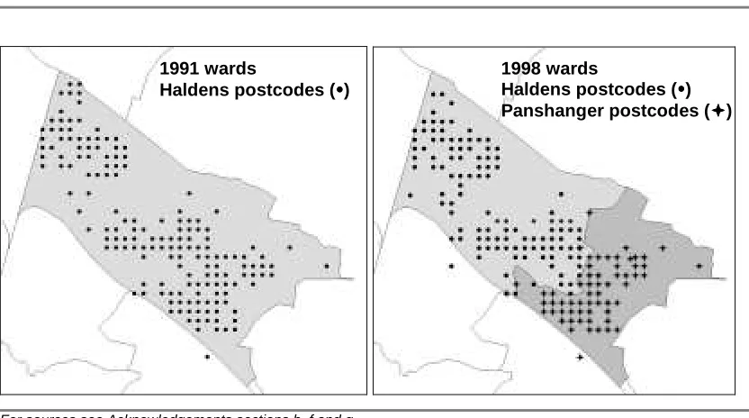
As noted in Figure 1, Haldens ward in Welwyn-Hatfield reduced in size between 1991
and 1998 with a new ward, Panshanger, being created. To illustrate the fit of a ward’s
constituent postcodes to the digital ward boundaries Figure 7 shows all the postcodes
for Haldens ward in 1991 with the 1991 ward boundary and the postcodes for Haldens
and Panshanger in 1998. The constituent postcodes for both wards in each year are, in
the main, consistent with the digital ward boundaries. However, two issues arise
relating to the 100m resolution of the postcode NGRs. Firstly a small number of
postcodes are located outside the correct ward boundary and secondly, many
postcodes which lie close together are given the same easting and northing
Figure 7: Constituent postcodes of wards in 1991 and 1998 (Haldens/Panshanger)
For sources see Acknowledgements sections b, f and g
Each quarter the Royal Mail’s latest Postal Address File (PAF) is made available to
ONS and provides the date of termination of postcodes no longer in use and the date
of introduction of new postcodes. Two to three thousand existing postcodes are
terminated each month and four to five thousand new postcodes are added (Yu and
Simpson 2000). Although the majority of change is due to business ‘large users’, the
termination and introduction of residential ‘small user’ postcodes can be taken as a
proxy for population change at a sub-ward level because when housing demolitions
occur postcodes are terminated, when newly built housing estates are constructed new
postcodes are allocated and when infill development occurs, the number of delivery
points is altered on the PAF (Penhale et al. 2000).
As previously noted, postcode-based LUTs are available to the academic community
via MIMAS that enable linkage between one geographical area and one time and
another (MIMAS 1999) and health professionals have access to similar information
through the NHS Postcode Directory, maintained on behalf of the Department of
1991 wards
Haldens postcodes ()
1998 wards
Health by ONS (ONS 2000). It should also be noted that many commercial
organisations supply postcode location information (see Martin and Higgs 1997). The
LUTs and the information relevant to the application are described below.
The Postcode-Enumeration District Directory (PCED) file provides a match between
postcodes and EDs in England and Wales. For every unit postcode there are details of
the EDs each postcode falls into, the number of resident households in each
postcode-ED intersection and the Ordnance Survey (OS) National Grid Reference (NGR)
(easting/northing). The directory was originally compiled with 1991 postcodes but has
been updated for 1995, 1996 and 1997 (Martin 1992; MIMAS 1999b). The Central
Postcode Directory (CPD) or Postzon file, originally created by the Department of
Transport, consists of a single data record for each UK postcode. The record contains
the NGR and local government and ward code for the first address in each postcode.
Additional information includes the date of introduction or termination and the
postcode user type (small or large). The CPD is available for 1991, 1993 and 1995
(Gatrell et al. 1991; MIMAS 1999b). The All Fields Postcode Directory (AFPD) is
the most recent addition to the LUTs at MIMAS and is the most comprehensive and
versatile. The AFPD is produced by ONS and combines data from the PCED and
various other LUTs produced by ONS to link postcodes to a wide range of
geographical units (MIMAS 1999b; Simpson and Yu 2000; Yu and Simpson 2000;
Simpson 2001).
Reviewing the documentation shows the files contain similar but not consistent
information. PCED and CPD files are both available in 1991 and 1995 but LUTs are
format as described previously. The PCED supports many to many links since
postcodes can be linked to more than one 1991 ED with an indication of weighting
given by the household count. The postcode-ward links given in the CPDs are on a
one to one best-fit basis for the years the files are available and AFPD postcode links
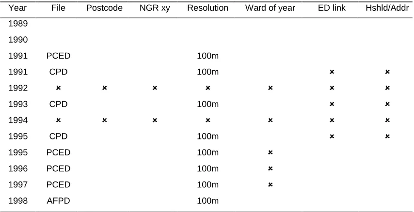
are also on a best-fit basis to the other geographies in the file. Table 3 summarises the
information availability relevant to establishing a consistent geography on a ward
[image:32.595.87.514.309.528.2]basis for the study period.
Table 3: Availability of relevant lookup table information
Year File Postcode NGR xy Resolution Ward of year ED link Hshld/Addr
1989
1990
1991 PCED 100m
1991 CPD 100m û û
1992 û û û û û û û
1993 CPD 100m û û
1994 û û û û û û û
1995 CPD 100m û û
1995 PCED 100m û
1996 PCED 100m û
1997 PCED 100m û
1998 AFPD 100m
For sources see Acknowledgements section f
5.2 ED Building-Brick approach to data conversion
The PCEDs for 1991 and more recent years and the AFPD for 1998 link postcodes of
the year of the file (the ‘year of interest’) back to the 1991 ED geography. The AFPD
also links the EDs forward to the 1998 ward geography. These LUTs can therefore be
used to develop a hybrid between the ‘freeze history’ and the ‘update to contemporary
zones’ approaches to establishing a consistent geography. The principle of the
approach being to use the constituent postcodes of a ward in a particular year and
GCTs and then to rebuild the data using another set of GCTs to the 1998 ward
geography. This is illustrated in Figure 8 whereby in a particular year two
hypothetical wards, North and South, are linked to various 1991 EDs. Whilst each
ward entirely overlaps three EDs, ED4 and ED5 are intersected by both. By 1998 East
and West wards have been created each overlapping various whole EDs but both
intersecting ED3. Data from North and South wards would be disaggregated into the
ED geography using postcode-derived weights to estimate each area of overlap and
[image:33.595.93.515.339.588.2]then reaggregated from EDs to the 1998 geography in a similar manner.
Figure 8: ED Building-Brick data disaggregation-reaggregation approach
It is necessary then to obtain data from the three sets of national LUTs available at
MIMAS that will indicate the number of postcodes in each ward of the year of
interest, a linkage to the 1991 ED geography and a count of households at each
postcode. Since the population estimation and SMR input files relate to electoral
Table 3, the three sets of national LUTs available at MIMAS contain similar but not
consistent information. Data relating to the study region must be extracted from the
national LUTs, area linkages must be established and any missing information
estimated. The stages necessary to achieve this are discussed below.
Stage 1. Obtain national postcode LUTs. As previously noted, the PCEDs, CPDs and
AFPD are available to the academic community via MIMAS. These were downloaded
from the server once necessary permissions were set up (see MIMAS 1999 and
Acknowledgements section f). The files held as a result are the PCED for 1991, 95, 96
and 97, the CPD for 1991, 93 and 95 and the AFPD for 1998 and will be referred to
below using a prefix of the LUT name and a two digit suffix for the year (e.g. CPD95)
Stage 2. Obtain digital boundary data for the study region. ED polygon boundaries
and boundaries for the six counties that comprise the region (Bedfordshire,
Cambridgeshire, Essex, Hertfordshire, Norfolk and Suffolk) were downloaded from
EDINA’s UKBORDERS website (see UKBORDERS 2001 and Acknowledgements
section b). The internal county boundaries were dissolved in the GIS package
ArcView to create an external digital boundary for the whole of Eastern Region.
Stage 3. Create GIS point covers for all national LUTs. For each file, the OS NGRs
for each postcode were used to locate each as a point in ArcView. The NGR ten digit
easting/northing coordinates given for the postcodes in the national LUTs do not
match the map unit measurements of the GIS region and ED polygon coverages. This
Stage 4. Abstract LUT data for Eastern Region. Two approaches can be taken to
select data for the study region from the national files. One is to select data records
that match a given criteria and the other is to select point locations that fall within the
external boundary of the region; both are possible using ArcView. The CPD and
AFPD files include a reference to the county each postcode is associated with in the
postcode point cover’s attribute table (the GIS database of fields and records) and the
relevant records can be selected from the table using logical queries. This approach is
not possible with the PCED files as the geographical codes only relate to 1991 and not
to later years. The postcode points that are located within the study region digital
boundary can be selected from the national file using a GIS ‘point in polygon’
operation (a GIS geometrical calculation, see Martin 1996). GIS point in polygon
does not give the same results as a database logical query as the postcode NGR 100m
resolution locates some study region points outside and some unwanted postcodes
inside the study region polygon (as previously noted in Figure 7). A comparison of the
county lookups and point in polygon approaches carried out on the CPD95 file shows
this applies to only a small number of points (112 out of 133271 postcodes) but is a
potential source of error.
Stage 5. Delete invalid postcodes. Postcodes are deemed invalid to the application in
various circumstances and are deleted from the files using logical queries on the
attribute tables. Postcode records are deleted where the postcode is terminated prior to
the year of interest and if the postcode is not yet introduced by the year (new
postcodes for 1999 are given in the AFPD98). Postcodes are also deleted when
designated as ‘large users’ since these are assumed to be business premises and it is
Stage 6. Establish postcode to ward of the year of interest links for all LUTs. This
information is needed to determine the postcode constituents of each ward in any
year. On the PCED91, the CPD for all years and the AFPD98 each postcode has a link
to the ward of the year of interest. However, the equivalent links are not given on the
PCEDs for 1995, 96 and 97 so there is a need to estimate this information. For the
PCED95 information can be obtained from the CPD95 but for the 1996 and 1997
PCEDs data from other years must be used. To do this the assumption needs to be
made that if changes in sub-district ward structure have not occurred between years
then the postcode-ward attribute information will be applicable. On this basis since
the ward structure for 1995 is the same as in 1996, information from the CPD95 can
be assigned to the PCED96 and similarly as 1997 has the same wards as 1998
information for the PCED97 can be obtained from the AFPD98.
This is achieved in two steps. Firstly, where postcodes are valid across the years and
present in both files the ward codes are assigned where a match can be made.
Secondly, to estimate the information not assignable through postcode record
matching, GIS ‘point to nearest point’ spatial joins are used to transfer the ward
attributes of the postcode points in the LUT of one year to the postcodes in another.
This is achieved through a radial search from the coordinates of the postcodes in one
GIS point cover to the postcode points in another. The attribute data is transferred
from the nearest postcode point to the origin point of the search. The postcode record
matching was carried out between the PCED95 and CPD95 and for the LUTs of
adjacent years indicated above. Unmatched postcodes in the PCEDs were then
that this process took place over was between postcode points 141 metres apart
suggesting that large changes are unlikely to have occurred between the years where
the ward structure remained the same and that, although minor boundary changes may
be missed, the assumption of applicability of information between years is reasonable.
Stage 7. Establish postcode to ED links for all LUTs. This information is needed so
that the postcodes from the LUTs for each year can be related back to the 1991 ED
geography. ED lookups are given for all postcodes on the PCED and AFPD files but
in the CPD93 and CPD95, links to the 1991 ED geography are not given. GIS point in
polygon is used then to assign ED codes to the CPD postcode points. Since point in
polygon can give different results due to the NGR resolution for consistency this was
also carried out for all the PCED and AFPD files. On each file around twelve points
were not allocated to an ED using point in polygon because the points were located in
wide rivers. The original ED code was allocated for these where available, but for the
CPD93 and 95 these points were manually relocated into the nearest ED polygon. The
As a result of carrying out stages 1-7, the postcode-ward-ED links now contained in
[image:38.595.83.481.162.317.2]the LUTs for Eastern Region are summarised below in Table 4.
Table 4: Postcode-ward-ED linked lookup table variables
File Postcode Ward of year 1991 ED-link Hshlds/Addr
PCED91
CPD91 û
CPD93 û
CPD95 û
PCED95
PCED96
PCED97
AFPD98
Based on sources referenced in Acknowledgements sections b, c, d, e & f
A data shortage not addressed above is the unavailability of postcode LUTs at
MIMAS for 1989, 90, 92 and 94. In terms of the ward structure of the region, the
numbers and names of wards are i) the same in 1989 and 1990 as in 1991, ii) the same
structure in 1992 as in 1993 and iii) the same in 1994 as in 1995. Data from the years
that are available will be used for the years where information is missing. Other
unresolved inconsistencies between the LUTs are that i) for each postcode on the CPD
files there are no counts of households or addresses and ii) that household counts
(derived by ONS and included in the PCEDs) are a different entity to the residential
address counts (supplied by the Royal Mail and included on the AFPD) since an
address can contain multiple households. Whilst the household counts could be
assigned using postcode matching and the point to nearest point technique described
above it is a fine level of detail that would need to be assumed applicable across years,
and given the different definitions for households and addresses, at this stage the
using just the postcode counts rather than postcode counts qualified by
household/address counts.
5.2.1 Ward and ED lookup files
To enable matching the postcode LUT records to wards, a year by year ‘pedigree’ of
the number, names and reference codes of each ward must be constructed. The ward
names and codes from the 1991 Census populations files and the electoral and Vital
Statistics (VS) files 1989-1998 have been combined along with the ward LUTs
supplied with the CPD and AFPD so that comparisons can be made (for sources of
these files see Acknowledgements sections c to f). This indicates when changes in
numbers of wards occur during the study period and reveals that the different input
data sources have inconsistent names and reference codes despite the definitive
information being available in Statutory Instruments (HMSO 1987-2001) when wards
are created or have boundary alterations.
Discrepancies in the numbers of wards exist between the electorates and VS. These
have been made consistent after consultation with the local authorities concerned. In
1991 the census populations show 1182 wards whereas the 1991 electorates and VS
have 1184. This relates to the Census Local Base Statistics (LBS) and data being
suppressed in small wards for confidentiality reasons (Cole 1994). For the population
estimates, rather than the Census LBS being used as a base population, the EWCPOP
1991 mid-year estimates will be used and the EWCPOPs are also two wards short of
the other data sources. Investigation of all the ward files reveals a wide variety of
codings, conventions and spellings confirming the ONS (2000) view that there is a
pedigree for the study period is a time-consuming clerical task. A summary of the
[image:40.595.84.476.164.201.2]ward numbers is given in Table 5.
Table 5: Ward numbers in the 1989-98 ward pedigree
Year 1989 to 1991 1992 to 1996 1997 to 1998
Number of wards 1184 1185 1192
For sources see Acknowledgements sections c, d & e
In addition to ward pedigree files, an ED lookup file is needed. Since the
point-in-polygon technique has been used, a point-in-polygon-based ED list is needed and this can be
obtained from the attribute table of the GIS ED coverage. A list of ED codes derived
in this way shows 11155 polygons with 11082 unique codes attached. There are
multiple polygons as some EDs are split by rivers and some include islands along the
region’s coastline. The GIS attribute table forms the basis of an ED lookup table for
matching records to the postcode LUTs.
5.2.2 Calculating GCT weights for data disaggregation-reaggregation
The information in the postcode-ward-ED LUTs is to be used to calculate overlap
weights for the intersections between the source and target geographies so that GCTs
can be used to adjust the ward input data for the years 1989-98 to the 1998 geography.
The hybrid freeze history and update to contemporary zones approach means that
effectively the source to target adjustments are carried out twice. First, the source
geography is the ward geography of the year of interest and the 1991 EDs are an
interim target geography and second, the EDs become the source geography and the
Three algorithms are outlined in Figures 9 to 11. The first algorithm shows how the
weights are calculated for the intersections between the source geography wards for
the year of interest and the target 1991 ED geography. The second algorithm
illustrates how weights are calculated to indicate the intersections between the source
1991 EDs with the target 1998 ward geography is essence reverse engineering the first
algorithm. The third algorithm outlines how GCTs will be used to disaggregate the
source data for each year of interest to create estimates in the 1991 ED geography and
then how a single GCT will be applied to rebuild the ED estimates for each year into
[image:41.595.90.506.533.734.2]the 1998 ward geography.
Figure 9: Algorithm to calculate ‘freeze history’ source-target GCT1 weights
Step Procedure
1 Upload the LUT for Eastern Region for the year of interest (e.g. PCED91)
2 Count the number of constituent postcodes in each source ward in the year of interest (e.g.
postcodes in Haldens ward 1991, below left)
3 Count postcode intersections with 1991 ED target geography (e.g. Haldens postcodes 1991
with 1991 EDs, below right)
4 Divide postcode-ED intersection count by ward constituent postcode count
5 The result is the source-target geography disaggregation weight, the proportion of the source
geography ward of the year of interest intersecting with each 1991 ED, the interim target
geography
For sources see Acknowledgements sections b, c, d, e & f
Haldens constituent postcodes 1991
Figure 10: Algorithm to calculate ‘update to contemporary zones’ source-target GCT2
weights
Step Procedure
1 Apportion sample data from the target 1998 geography to 1991 ED geography using GCT
disaggregation weights calculated above
2 Sum the disaggregated target geography estimated in 1991 ED geography
3 Divide the GCT disaggregated target ward-source ED geography intersections by the total ED
estimate
4 The result is the proportion of each source ED intersecting with a target 1998 ward (which will
take a value of more than zero but less than or equal to one)
Figure 11: Algorithm to use GCTs to carry out data disaggregation-reaggregation
process
Step Procedure
1 Upload source geography ward data for year of interest (e.g. deaths data for 1991 Haldens
ward)
2 Use GCT1 to estimate source to 1991 ED interim target geography intersections by
multiplying ward data by GCT weights (e.g. deaths data for 1991 Haldens ward disaggregated
into intersection counts)
3 Aggregate intersection counts into interim target ED totals (e.g. deaths data for 1991 Haldens
ward estimated for 1991 ED geography)
4 Use GCT2 to apportion ED geography to target 1998 geography using source-target weights
(e.g. deaths data for 1991 Haldens ward estimated for 1991 ED geography is reaggregated to
1998 geography Haldens and Panshanger wards)
5.2.3 ED Building-Brick derived consistent geography: assessing the output
The algorithms as outlined above have been programmed in FORTRAN 90 to
produce GCTs for 1991, 1993 and 1995 to 1998, the years for which the
postcode-ward-ED LUTs have been assembled. To test the programs and assess their output
hypothetical ward populations have been used as input data. The total study region
population has been set at 1,192,000 divided equally in the source geographies
between the 1,184 wards in 1990 and 1991, the 1,185 wards in 1992-96 and the 1,192
The hypothetical ward data have been disaggregated and reaggregated from source to
target geographies to be consistent with 1998 geography using the GCTs. Since there
are PCED and CPD files duplicating 1991 and 1995 and some years missing (1989,
90, 92 and 94), there are eight output files relating to six out of the nine years of the
study period. For the study region as a whole in every year (i.e. the years the
procedure has been programmed) the total population is disaggregated and
reaggregated back to within a few decimal places so that no whole persons are lost
from the system. The ward geography for 1998 disaggregates and reaggregates almost
perfectly but this is to be expected as the reaggregation weights are based on its own
disaggregation weights.
The program outputs can be assessed through graphs to show the size of each ward
population once adjusted to 1998 geography and choropleth maps to identify the
locations where large differences have been found to occur for the interim ED
geography and for the 1998 target geography. Any differences identified between
source to target GCT adjusted data can be due to genuine changes in ward size and
structure, incorrect LUT links between geographical areas or incorrect assumptions,
method or programming.
Figure 12 shows the output of each of the programs with the hypothetical populations
adjusted to the 1998 geography. If the GCTs are estimating the geographical changes
correctly then any counts of less than 1,000 on the graph represent wards that have
reduced in size by 1998 and wards that have increased for counts of over 1,000.
Whilst there is much clustering around 1,000 persons per ward there are many large
Figure 12: Adjustment of hypothetical populations to 1998 geography, ED version 1
Figure 13: Proportional change of ward populations 1997-98
[image:44.595.94.510.386.727.2]To identify locations where excessive year by year adjustments have occurred, the
population counts adjusted to 1998 geography in one year were divided by the count
for the next. The results of these calculations were choropleth mapped using the 1998
ward boundaries with the largest differences observed between 1997 and 1998
especially in the north-west of the region (see Figure 13). This is unexpected because
the ward structure did not change between these years suggesting, together with other
large year to year changes, that there are some problems in the geographical links in
the GCTs.
Investigation of the GCTs and input files showed some differences in ward code
conventions that had not previously been identified. The 1998 ward codes in the
AFPD vary between six and four figure alphanumeric codes whereas the elector and
VS files use six figure throughout. These were rationalised to give consistency
between the postcode-ward-ED LUTs and the ward data input files. The programs to
calculate the GCTs were re-run and the hypothetical population counts adjusted to the
1998 geography using the new GCTs. For 1991 and 1995, since LUT information is
available from both the PCED and CPD an average of the data estimated to 1998
Figure 14: Adjustment of hypothetical populations to 1998 geography, ED version 2
The output in Figure 14 has a more marked clustering for each ward around 1,000
persons than was previously shown. There are still wards with populations well above
and below 1,000 and these should represent wards that have respectively increased or
decreased in size between source and target ward geographies. The locations of the
largest adjustments have been identified to determine whether these represent
substantial changes in the ward boundaries over time or error. For wards in the local
authority district Welwyn-Hatfield, previously noted as experiencing boundary
changes during 1991 (see Figure 1), bars on the graph above the 1000 person level
include Welwyn South and Brookmans Park and Little Heath, both of which have
larger areal extents than the previous boundary definitions. Similarly wards which
reduced in size over time, Welwyn North, Haldens and Hatfield East are represented
on the graph by bars below the 1000 person level. Other locations with large changes
in hypothetical populations are Peterborough and Thurrock which both became
Unitary Authorities by 1998 experiencing substantial changes to their constituent
wards. These are illustrated in Figure 15, wards with no boundary changes marked
[image:47.595.92.515.200.579.2]with an X.
Figure 15: Ward boundaries 1991 and 1998, Thurrock and Peterborough Unitary
Authorities
For sources see Acknowledgements section b & g
As previously noted, many of the larger year by year variations identified are in
locations where ward boundaries known to have changed. However, variation will be
due to aspects of the postcode-ward-ED linkage approach that relate to the postcode
NGR resolution and point in polygon-derived links. Further checks on the method can
aggregated into the wards those EDs comprise. These ward populations can then be
adjusted to the 1998 geography with the interim ED estimates output so that they can
[image:48.595.89.508.187.340.2]be checked against the original SAS ED populations.
Figure 16 Estimated and original ED and ward populations
The scatterplot on the left in Figure 16 shows the estimated ED populations plotted
against the original ED populations from the SAS. Although statistically significant
(p-value 0.000), there is a correlation of just 0.347 between the estimated and original
populations. When these estimated ED populations are aggregated into 1991 wards
the result is a closer match between the estimated and original ward populations with
a correlation of 0.982 (p-value 0.000). This suggests that whilst the method is not a
good estimator of ED populations, ward-level populations are estimated well.
However, if populations are incorrectly allocated to EDs, difficulties may occur when
part EDs are apportioned to the 1998 geography.
Various problems relating to the postcode resolution and point in polygon technique
will lead to poor estimates of ED populations. As previously noted a postcode can be
allocated to an incorrect ED because the NGR locates it the wrong side of a boundary.
The stacking of postcode coordinates can lead to some EDs having an over-allocation