Beyond Local Nash Equilibria
for Adversarial Networks
∗
Frans A. Oliehoek
Rahul Savani
Jose Gallego
Elise van der Pol
Roderich Groß
June 20, 2018
Abstract
Save for some special cases, current training meth-ods for Generative Adversarial Networks (GANs) are at best guaranteed to converge to a ‘local Nash equilibrium’ (LNE). Such LNEs, however, can be arbitrarily far from an actual Nash equilibrium (NE), which implies that there are no guarantees on the quality of the found generator or classifier. This paper proposes to model GANs explicitly as finite games in mixed strategies, thereby en-suring that every LNE is an NE. With this for-mulation, we propose a solution method that is proven to monotonically converge to a resource-bounded Nash equilibrium (RB-NE): by increas-ing computational resources we can find better solutions. We empirically demonstrate that our method is less prone to typical GAN problems such as mode collapse, and produces solutions that are less exploitable than those produced by GANs and MGANs, and closely resemble theo-retical predictions about NEs.
1. Introduction
Generative Adversarial Networks (GANs) (Goodfellow et al., 2014) are a framework in which two neural networks compete with each other: thegenerator (G)tries to trick theclassifier (C)into classifying its generated fake data as true. GANs hold great promise for the development of accurate generative models for complex distributions. Con-sequently, in just a few years, GANs have grown into a major topic of research in machine learning. A core appeal is that they do not need to rely on distance metrics (Li et al., 2016). However, GANs are difficult to train (Unterthiner et al., 2018; Arjovsky and Bottou, 2017; Arjovsky et al., 2017). A typical problem ismode collapse, which can take the form ofmode omission, where the generator does not produce points from certain modes, ormode degeneration,
∗
This version supersedes our earlier arXiv paper (Oliehoek et al., 2017).
in which for at least one mode the generator only partially covers the mode. Moreover, while learning the players may forget: e.g., it is possible that a classifier correctly learns to classify part of the input space as ‘fake’ only to forget this later when the generator no longer generates examples in this part of space. In fact, except for very special cases (cf. Section 7), the best current training methods can offer (Heusel et al., 2017; Unterthiner et al., 2018) is a guarantee to converge to alocalNash equilibrium (LNE) (Ratliff et al., 2013). However, an LNE can be arbitrarily far from an NE (which we will also refer to as ‘global NE’ to discriminate) and the corresponding generator might be exploitable by a strong opponent due to suffering from problems such as mode collapse. Moreover, adding computational resources alone may not offer a way to escape these local equilibria: the problem does not lie in the lack of computational re-sources, but is inherently the result of only allowing small steps in strategy space using gradient-based training. We introduce a novel approach that does not suffer from getting trapped in LNEs: finiteGenerative Adversarial Net-work Games (GANGs)formulate adversarial networks as finitezero-sum games, and the solutions that we try to find are saddle points inmixed strategies. This approach is moti-vated by the observation that, considering a GAN as a finite zero-sum game, in the space of mixed strategies, any local Nash equilibrium is a global one. Intuitively, the reason for this is that whenever there is a profitable pure strategy deviation one can move towards it in the space of mixed strategies.
Since we cannot expect to find exact best responses due to the extremely large number of pure strategies that result for sensible choices of neural network classes, we introduce resource-bounded best-responses (RBBRs), and the cor-responding resource-bounded Nash equilibrium (RB-NE), which is a pair of mixed strategies in which no player can find a better RBBR. This is richer than the notion of local Nash equilibrium in that it captures not only failures of es-caping local optima of gradient descent, but applies toany approximate best response computations, including methods with random restarts, and allows us to provide convergence guarantees.
The key features of our approach are that:
• It is based on finite zero-sum games, and as such it enables the use of existing game-theoretic methods. In this paper we focus on one such method, Parallel Nash Memory (PNM) (Oliehoek et al., 2006).
• It will not get trapped in LNEs: we prove that it mono-tonically converges to an RB-NE, which means that more computation can improve solution quality.
• Moreover, it works for any network architecture (unlike previous approaches, see Section 7). In particular, future improvements in classifiers/generator networks can be exploited directly.
We investigate empirically the effectiveness of PNM and show that it can indeed deal well with typical GAN prob-lems such as mode collapse and forgetting, especially in distributions with asymmetric structure to their modes. We show that the found solutions are much less susceptible to being exploited by an adversary, and that they more closely match the theoretical predictions made by Goodfellow et al. (2014) about the conditions at a Nash equilibrium.
2. Background
We defer a more detailed treatment of related work on GANs and recent game-theoretic approaches until Section 7. Here, we introduce some basic game-theoretic notation.
Definition 1 (‘game’). A two-player strategic game, which we will simply call ‘game’, is a tuple
D,{Si}i∈D,{ui}i∈D
, whereD = {1,2} is the set of players,Siis the set ofpure strategies(actions) for playeri,
andui:S →Risi0spayoff function defined on the set of
pure strategy profilesS :=S1× S2. When the action sets
are finite, the game isfinite.
We also writesiands−ifor the strategy of agentiand its
opponent respectively.
A fundamental concept is the Nash equilibrium (NE), which is a strategy profile such that no player can unilaterally deviate and improve his payoff.
Definition 2 (Pure Nash equilibrium). A pure strategy profile s = hsi, s−ii is an NE if and only if ui(s) ≥ ui(hs0i, s−ii)for all playersiands0i∈ Si.
A finite game may not possess a pure NE. Amixed strategy µi of playeri is a probability distribution over i’s pure
strategiesSi. The set of such probability distributions is
denoted by∆(Si). The payoff of a player under a profile of
mixed strategiesµ=hµ1, µ2iis defined as the expectation:
ui(µ) :=Ps∈S[ Q
j∈Dµj(sj)]·ui(s).
Then an NE in mixed strategies is defined as follows.
Definition 3(Mixed Nash equilibrium). Aµ=hµi, µ−ii
is an NE if and only ifui(µ)≥ui(hs0i, µ−ii)for all players iand potential unilateral deviationss0i ∈ Si.
Every finite game has at least one NE in mixed strate-gies (Nash, 1950). In this paper we deal with two-player zero-sumgames, whereu1(s1, s2) = −u2(s1, s2)for all
s1∈ S1, s2∈ S2. The equilibria of zero-sum games, also
calledsaddle points,1have several important properties, as stated in the Minmax theorem.
Theorem 1(von Neumann (1928)). In a finite zero-sum game,minµ2maxµ1u1(µ) = maxµ1minµ2u1(µ) = v
∗,
wherev∗is thevalueof the game.
All equilibria have payoff v∗ and equilibrium strategies are interchangeable: ifhµ1, µ2iandhµ01, µ02iare equilibria,
then so arehµ01, µ2iandhµ1, µ02i(Osborne and Rubinstein,
1994). This means that in zero-sum games we do not need to worry about equilibrium selection: any equilibrium strat-egy for a player is guaranteed to achieve the value of the game. Moreover, the convex combination of two equilibria is an equilibrium, meaning that the game has either one or infinitely many equilibria.
We also employ the standard, additive notion ofapproximate equilibrium:
Definition 4. A pair of (possibly pure) strategies(µi, µ−i)
is an-NE if∀i ui(µi, µ−i)≥maxµ0
iui(µ
0
i, µ−i)−.In
other words, no player can gain more thanby deviating.
In the literature, GANs have not typically been considered as finite games. The natural interpretation of the standard setup of GANs is of an infinite game where payoffs are defined over all possible weight parameters for the respective neural networks. With this view we do not obtain existence of saddle points in the space of parameters2, nor the desirable properties of Theorem 1. Some results on the existence of saddle points in infinite action games are known, but they require properties like convexity and concavity of utility functions (Aubin, 1998), which we cannot apply as they would need to hold w.r.t. the neural network parameters. This is why the notion oflocal Nash equilibrium (LNE)has arisen in the literature (Ratliff et al., 2013; Unterthiner et al., 2018). Roughly, an LNE is a strategy profile where neither player can improve in a small neighborhood of the profile.3
1Note that in game theory the term ‘saddle point’ is used to
denote a ‘global’ saddle point which corresponds to a Nash equi-librium: there is no profitable deviation near or far away from the current point. In contrast, in machine learning, the term ’sad-dle point’ typically denotes a ‘local’ sad’sad-dle point: no player can improve its payoff by making a small step from the current joint strategy.
2Note that Goodfellow et al. (2014)’s theoretical results on the
existance of an equilibrium are “done in a non-parametric setting” which studies “convergence in the space of probability density functions”, not parameters.
In finite games every LNE is an NE, as, whenever there is a global deviation (i.e., a better response), one can always deviate locally in the space of mixed strategies towards a pure best response (by playing that better response with higher probability).
3. GANGs
In order to capitalize on the insight that we can escape local equilibria by switching to mixed strategy space for a finite game, we formalize adversarial networks in a (finite) games setting, that we call (finite)Generative Adversarial Network Games (GANGs).
We start with making explicit how general (infinite) GANs correspond to strategic games, via the GANG framework:
Definition 5 (GANG). A GANG is a tuple M =
hpd,hG, pzi, C, φiwith
• pd(x)is the distribution over (‘true’ or ‘real’) data points x∈Rd.
• Gis a neural network class parametrized by a parameter vectorθG ∈ ΘG anddoutputs, such that G(z;θG) ∈
Rddenotes the (‘fake’ or ‘generated’) output ofGon a
random vectorzdrawn from some distributionz∼pz. • Cis a neural network class parametrized by a parameter
vectorθC∈ΘCand a single output, such that the output C(x;θC)∈[0,1]indicates the ‘realness’ ofxaccording
toC.
• φ: [0,1]→R is a measuring function (Arora et al.,
2017)—e.g., log for GANs, the identity mapping for WGANs—used to specify game payoffs, explained next.
A GANG induces a zero-sum game in an intuitive way:
Definition 6. The induced zero-sum strategic-form game of a GANG ishD={G, C},{SG,SC},{uG, uC}iwith:
• SG={G(·;θG)|θG∈ΘG}the set of strategiessG; • SC={C(·;θC)|θC∈ΘC}, the set of strategiessC; • uC(sG, sC) = Ex∼pd[φ(sC(x))] −
Ez∼pz[φ(sC(sG(z)))]. I.e., the score of C is the
expected ‘measured realness’ of the real data minus that of the fake data;
• uG(sG, sC) =−uC(sG, sC).
As such, when usingφ = log, GANGs employ a payoff function forGthat use Goodfellow et al. (2014)’s trick to enforce strong gradients early in the training process, but it applies this transformation touCtoo, in order to retain the
zero-sum property. The correctness of these transformations are proven in Appendix A.
In practice, GANs are represented using floating point
num-bers, of which, for a given setup, there is only a finite (albeit large) number. In GANGs, we formalize this:
Definition 7. Any GANG whereG, Care finite classes— i.e., classes of networks constructed from a finite set of node types (e.g., {Sigmoid, ReLu, Linear})—and with architec-tures of bounded size, is called afinite network class GANG. A finite network class GANG in which the setsΘG,ΘCare
finite too, it is called afinite GANG.
From now on, we will focus on finite GANGs. We empha-size this finiteness, because this is exactly what enables us to obtain the desirable properties mentioned in Section 2: existence of (one or infinitely many) mixed NEs with the same value, as well as the guarantee that any LNE is an NE. Moreover, these properties hold for the GANG in its origi-nal formulation—not for a theoretical abstraction in terms of (infinite capacity) densities—which means that we can truly expect solution methods (that operate in the paramet-ric domain) to exploit these properties. However, since we do not impose any additional constraints or discretization4, the number of strategies (all possible unique instantiations of the network class with floating point numbers) ishuge. Therefore, we think that finding (near-) equilibria with small supports is one of the most important challenges for making principled advances in the field of adversarial networks. As a first step towards addressing this challenge, we propose to make use of theParallel Nash Memory (PNM)(Oliehoek et al., 2006), which can be seen as a generalization (to non-exact best responses) of thedouble oracle method (McMa-han et al., 2003).
4. Resource-Bounded GANGs
While finite GANGs do not suffer from LNEs, solving them is non-trivial: even though we know that there always is a direction (i.e., a best response) that we can play more frequently to move towards an NE, computing that direction itself is a computationally intractable task. There is huge number of candidate strategies and the best-response payoff is a non-linear (or convex) function of the chosen strategy. This means that finding an NE, or even an−NE will be typically beyond our capabilities. Therefore we consider players with bounded computational resources.
Resource-Bounded Best-Responses (RBBR). A Nash equilibrium is defined by the absence of better responses for any of the players. As such, best response computation is a critical tool to verify whether a strategy profile is an NE,
4
Therefore, our finite GANGs have the same representational capacity as normal GANs that are implemented using floating point arithmetic. When strategies would be highly non-continuous functions ofθGandθC, then a discretization (e.g., a floating point
and is also a common subroutine in algorithms that compute an NE.5However, since computing an (-)best response will generally be intractable for GANGs, we examine the type of solutions that we actually can expect to compute with bounded computational power by the notion of resource-bounded best responseand show how it naturally leads to theresource-bounded NE (RB-NE)solution concept. We say thatSRB
i ⊆ Siis the subset of strategies of player i, thatican compute as a best response, given its bounded computational resources. This computable set is an abstract formulation that can capture gradient descent being trapped in local optima, as well as other phenomena that prevent us from computing a best response (e.g., not even reaching a local optimum in the available time).
Definition 8. A strategysi∈ SiRBof playeriis a
resource-bounded best-response(RBBR) against a (possibly mixed) strategyµj, if∀s0i∈ S
RB
i , ui(si, µj)≥ui(s0i, µj).
That is,sionly needs to be amongst the best strategies that
playerican computein response toµj. We denote the set
of such RBBRs toµjbyS
RBBR(µj)
i ⊆ S
RB i .
Definition 9. Aresource-bounded best-response function fRBBR
i : ∆(Sj)→ SiRBis a function that maps from the
set of possible strategies of playerjto an RBBR fori, s.t.
∀µj f
RBBR
i (µj)∈ S
RBBR(µj)
i .
Using RBBRs, we define an intuitive specialization of NE:
Definition 10. µ=hµi, µjiis aresource-bounded NE
(RB-NE)iff∀i ui(µi, µj)≥ui(fiRBBR(µj), µj).
That is, an RB-NE can be thought of as follows: we present µ to each player i and it gets the chance to switch to another strategy, for which it can apply its bounded re-sources (i.e., usefRBBR
i ) exactly once. After this
applica-tion, the player’s resources are exhausted and if the found fiRBBR(µj)does not lead to a higher payoff it will not have
an incentive to deviate.6
Clearly, an RB-NE can be linked to the familiar notion of-NE by making assumptions on the power of the best response computation.
5
We motivate the need for an alternative solution concept. We acknowledge the fact that there are solution methods that do not require the explicit computation for best responses, but are not aware of any such methods that would be scalable to the huge strategy spaces of finite GANGs.
6
Of course, during training the RBBR functions will be used many times, and therefore the overall computations thatwe, the de-signers (‘GANG trainers’),use is a multitude of the computational capabilities that that the RB-NE assumes. However, this is of no concern: the goal of the RB-NE is to provide a characterization of the end point of training. In particular, it allows us to give an ab-stract formalization of the idea that more computational resources imply a better solution.
Theorem 2. If both players are powerful enough to compute -best responses, then an RB-NE is an-NE.
Proof. Starting from the RB-NE (µi, µj), assume an
arbitrary i. By definition of RB-NE ui(µi, µj) ≥ ui(fiRBBR(µj), µj)≥maxµ0
iui(µ
0
i, µj)−.
Non-deterministic Best Responses. The above defi-nitions assumed deterministic RBBR functions fRBBR
i .
However, in many cases the RBBR function can be non-deterministic (e.g., due to random restarts), which means that the setsSRB
i are non-deterministic. This is not a
fun-damental problem, however, and the same approach can be adapted to allow for such non-determinism.
In particular, now letfRBBR
i be a non-deterministic
func-tion, anddefineSRB
i as the range of this function. That
is, we defineSRB
i as that set of strategies that our
non-deterministic RBBR function might deliver. Given this mod-ification the definition of the RB-NE remains unchanged: a strategy profileµ=hµi, µjiis anon-deterministic RB-NE
if each playeriuses all its computational resources by call-ingfRBBR
i (µj)once, and no player finds a better strategy
to switch to.
5. Solving GANGs
Treating GANGs as finite games in mixed strategies permits building on existing tools and algorithms for these classes of games (Fudenberg and Levine, 1998; Rakhlin and Sridharan, 2013a; Foster et al., 2016). In this section, we describe how to use the Parallel Nash Memory (Oliehoek et al., 2006), which explicitly aims to prevent forgetting, is particularly tailored to finding approximate NEs with small support, and monotonically7converges to such an equilibrium.
In the following, we give a concise description of a slightly simplified form of Parallel Nash Memory (PNM) and how we apply it to GANGs. For ease of explanation, we focus on the setting with deterministic best responses.8
The algorithm is shown in Algorithm 1. Intuitively, PNM
7
For an explanation of the precise meaning of monotonic here, we refer to Oliehoek et al. (2006). Roughly, we will be ‘secure’ against more strategies of the other agent with each iteration. This does not imply that the worst case payoff for an agent also improves monotonicaly. The latter property, while desirable, is not possible with an approach that incrementally constructs sub-games of the full game, as considered here: there might always be a part of the game we have not seen yet, but which we might discover in the future that will lead to a very poor worst case payoff for one of the agents.
8
In our experiments, we use random initializations for the best responses. To deal with this non-determinism we simply discard any tests that are not able to find a positive payoff over the current mixed strategy NEhµG, µCi, but we do not terminate. Instead, we
Algorithm 1PARALLELNASH MEMORY FOR GANGS
WITH DETERMINISTICRBBRS
1: hsG, sCi ←INITIALSTRATEGIES()
2: hµG, µCi ← h{sG},{sC}i .set initial mixtures
3: whileTruedo
4: sG←RBBR(µC) .get new bounded best resp.
5: sC←RBBR(µG)
6: // Expected payoffs of these ‘tests’ against mixture: 7: uBRs←uG(sG, µC) +uC(µG, sC)
8: ifuBRs≤0then
9: break
10: end if
11: SG←AUGMENTGAME(SG, sG, sC)
12: hµG, µCi ←SOLVEGAME(SG)
13: end while
14: returnhµG, µCi .found an BR-NE
incrementally grows a strategic gameSG, over a number of iterations, using the AUGMENTGAMEfunction. It uses SOLVEGAMEto compute (via linear programming, see, e.g., Shoham and Leyton-Brown (2008)) a mixed strategy NE
hµG, µCiof this smaller gameat the end of each iteration.
In order to generate new candidate strategies to include in SG, at the beginning of each iteration the algorithm uses a ‘search’ heuristic to deliver new promising strategies. In our GANG setting, we use the resource-bounded best-response (RBBR) functions of the players for this purpose. After having found new strategies, we test if they ‘beat’ the currenthµG, µCi, if they do,uBRs > 0, and the game is
augmented with these and solved again to find a new NE of the sub-gameSG. If they do not,uBRs ≤0, and the
algorithm stops.9
In order to augment the game, PNM evaluates (by simula-tion) each newly found strategy for each player against all of the existing strategies of the other player, thus constructing a new row and column for the maintained payoff matrix. In order to implement the best response functions, any exist-ing neural network architectures can be used. However, we need to compute RBBRs againstmixturesof networks of the other player. ForCthis is trivial: we can simply generate a batch of fake data from the mixtureµG. Implementing an
RBBR forGagainstµC is slightly more involved, as we
need to back-propagate the gradient from all the different sC∈µCtoG. Intuitively, one can think of a combined
net-work consisting of theGnetwork with its outputs connected to everysC ∈ µC(see Figure 1). The predictionsyˆsC of
these componentssC∈µCare combined in a single linear 9
Essentially, this is the same as the double oracle method, but it replaces exact best-response computation with approximate RBBRs. Therefore, we refer to this as PNM, since that inherently allows for approximate/heuristic methods to deliver new ‘test’ strategies (Oliehoek et al., 2006). It also enables us to develop a version fornon-deterministicRBBRs, by literally adopting the PNM algorithm.
output nodeyˆ = P
sC∈µCµC(sC)·yˆsC. This allows us
to evaluate and backpropagate through the entire network. A practical implementation that avoids memory concerns instead loops through each componentsC∈µCand does
the evaluation of the weighted predictionµC(sC)·yˆsC and
subsequent backpropagation per component.
Intuitively, it is clear that PNM converges to an RB-NE, which we now prove formally.
Theorem 3. If PNM terminates, it has found an RB-NE.
Proof. We show thatuBRs≤0implies we have an RB-NE:
uBRs = uG(fGRBBR(µC), µC) +uC(µG, fCRBBR(µG))
≤ 0 =uG(µG, µC) +uC(µG, µC) (1)
Note that, per Def. 8,uG(fGRBBR(µC), µC)≥uG(s0G, µC)
for all computable s0G ∈ SRB
G (and similar for C).
Therefore, the only way that uG(fGRBBR(µC), µC) ≥ uG(µG, µC)could fail to hold, is ifµGwould include some
strategies that are not computable (not inSRB
G ) that
pro-vide higher payoff. However, as the support ofµGis
com-posed of strategies computed in previous iterations, this cannot be the case. We conclude uG(fGRBBR(µC), µC) ≥ uG(µG, µC) and similarly uC(µG, fCRBBR(µG)) ≥ uC(µG, µC). Together with (1) this directly implies uG(µG, µC) =uG(fGRBBR(µC), µC)anduC(µG, µC) = uC(µG, fCRBBR(µG)), indicating we found an RB-NE.
Corollary 1. Algorithm 1 terminates andmonotonically converges to an equilibrium.
Proof. This follows directly from the fact that there are only finitely many RBBRs and the fact that we never forget RBBRs that we computed before, thus the proof for PNM (Oliehoek et al., 2006) extends to Algorithm 1.
The PNM algorithm for GANGs is parameter free, but we mention two adaptations that are helpful.
Interleaved training of best responses. In order to speed up convergence of PNM, it is possible to train best responses ofGandCin parallel, givingGaccess to the intermediate results of fRBBR
C . This reduces the number of needed
PNM iterations, but does not seem to affect the quality of the found solutions, as demonstrated in Appendix D. The results shown in the main paper do not employ this trick.
. . . . .
Figure 1: Network architecture that allows gradients fromsC ∈µCto be back-propagated toG.
(both real and fake), and include these data points as ad-ditional fake data for trainingC. The number of ‘uniform fake points’ chosen coincides with the batch size used for training.
6. Experiments
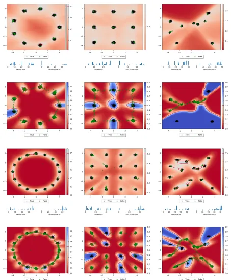
Here we report on experiments that aim to test if searching in mixed strategies with PNM-GANG can help in reducing problems with training GANs, and if the found solutions (near-RB-NEs) provide better generative models and are po-tentially closer to true Nash equilibria than those found by GANs (near-LNEs). Since our goal is to produce better gen-erative models, we refrain from evaluating these methods on complex data like images: image quality and log likelihood are not aligned as for instance shown by Theis et al. (2016). Moreover there is debate about whether GANs are overfit-ting (memorizing the data) and assessing this from samples is difficult; only crude methods have been proposed e.g., (Arora and Zhang, 2017; Salimans et al., 2016; Odena et al., 2017; Karras et al., 2018), most of which provide merely a measure of variability, not over-fitting. As such, we choose to focus on irrefutable results on mixture of Gaussian tasks, for which the distributions can readily be visualized, and which themselves have many applications.
Experimental setup. We compare our PNM approach (‘PNM-GANG’) to a vanilla GAN implementation and state-of-the-art MGAN (Hoang et al., 2018). Detailed training and architecture settings are summarized in the appendix. The mixture components comprise grids and annuli with equal-variance components, as well as non-symmetric cases with randomly located modes and with a random covariance matrix for each mode. For each domain we create test cases
with 9 and 16 components. In our plots, black points are real data, green points are generated data. Blue indicates areas that are classified as ‘realistic’ while red indicates a ‘fake’ classification byC.
Found solutions. The results produced by regular GANs and PNM-GANGs are shown in Figure 2 and clearly convey three main points:
1. The PNM-GANG mixed classifier has a much flatter surface than the classifier found by the GAN. Around the true data, the GANG classifier outputs around 0.5 indicating indifference, which isin line with the theoreti-cal predictionsabout the equilibrium (Goodfellow et al., 2014).
2. We see that this flatter surface is not coming at the cost of inaccurate samples. In contrast: nearly all samples shown are hitting one of the modes and thusthe PNM-GANG solutions are highly accurate, much more so than the GANs’ solutions.
3. Finally, the PNM-GANGs, unlike GANs,do not suffer from mode omission; they leave out no modes. We also note that PNM-GANG typically achieved these results with fewer total parameters than the regular GAN, e.g., 1463 vs. 7653 for the random 9 task in Figure 2.
This shows that, qualitatively, the use of multiple generators seems to lead to good results. This is corroborated by results we obtained using MGANs (illustrations and complete de-scription can be found in Appendix C.2), which only failed to represent one mode in the ‘random’ task.
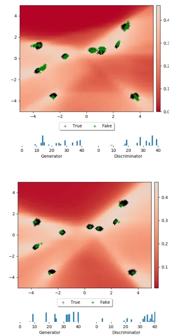
modes, however, not all modes arefullycovered. As also pointed out by Arjovsky et al. (2017), the best response ofG againstµCis a single point with the highest ‘realness’, and
therefore the WGAN they introduced uses fewer iterations forGthan forC. Inspired by this, we investigate if we can reduce the mode collapse by reducing the learning rate ofG. The results in Figure 3 show that more area of the modes are covered confirming this hypothesis. However, it also makes clear that by doing so, we are now generating some data outside of the true data, so this is a trade-off. We point out that also with total mode degeneration (where modes collapse to Dirac delta peaks), the PNM mechanism theo-retically would still converge, by adding in ever more delta peaks covering parts of the modes.
Exploitability of solutions. Finally, to complement the above qualitative analysis, we also provide a quantitative analysis of the solutions found by GANs, MGANs and PNM-GANGs. We investigate to what extent they are ex-ploitable by newly introduced adversaries with some fixed computational power (as modeled by the complexity of the networks we use to attack the found solution).
In particular, for a given solutionµ˜ = ( ˜µG,µ˜C)we use the
following measure of exploitability:
explRB( ˜µG,µ˜C),RBmaxµGuG(µG,µ˜C)
+RBmaxµCuC( ˜µG, µC), (2)
where ‘RBmax’ denotes an approximate maximization per-formed by an adversary of some fixed complexity.
That is, the ‘RBmax’ functions are analogous to thefiRBBR functions employed in PNM, but the computational re-sources of ‘RBmax’ could be different from those used for thefRBBR
i . Intuitively, it gives a higher score ifµ˜ is
easier to exploit. However, it is not a true measure of dis-tance to an equilibrium: it can return values that are lower than zero which indicate thatµ˜ could not be exploited by the approximate best responses.
Our exploitability is closely related to the use of GAN train-ing metrics (Im et al., 2018), but additionally includes the exploitability of the classifier. This is important: when only testing the exploitability of the generator, this does give a way to compare generators,but it does not give a way to assess how far from equilibirum we might be. Since finite GANGs are zero-sum games, distance to equilibrium is the desired performance measure. In particular, the exploitabil-ity of the classifier actually may provide information about the quality of the generator: if the generator holds up well against a perfect classifier, it should be close to the data distribution. For a further motivation of this measure of exploitability, please see Appendix B.2.
[image:8.612.333.510.67.411.2]We perform two experiments on the 9 random modes task;
Figure 3: Results for PNM with a learning rate of7−4for
the generator (top). Compare with previous result (bottom, duplicated from the first row of Figure 2).
results for other tasks are in Appendix C.2. First, we in-vestigate the exploitability of solutions delivered by GANs, MGANs and GANGs of different complexities (in terms of totalnumber of parameters used). For this, we compute ‘at-tacks’ (approximate best responses) to these solutions using attackers of fixed complexity (a total of 453 parameters for the attackingGandCtogether).
Figure 4: Exploitability results for the nine randomly located modes task. Left: exploitability of PNM-GANGs of various complexities (indicated numbers) found in different iterations. Middle: comparison of exploitability of PNM-GANGs, GANs and MGAN of various complexities. Right: exploitability of PNM-GANGs, GANs and MGAN, when varying the complexity of the attacking ‘RBmax’ functions. Complexities are expressed in total number of parameters (forGandC together). See text for detailed explanation of all.
Note that here the x-axis shows the complexity in terms of total parameters. The figure shows an approximately monotonic decrease in exploitability for GANGs for in-creasing number of parameters, while GANs and MGANs with higher complexity are still very exploitable. In con-trast to GANGs, more complex architectures for GANs or MGANs are thus by no means a way to guarantee a better solution.
Secondly, we investigate what happens for the converged GAN / PNM-GANG solution of Figure 2, which have com-parable complexities, when attacked with varying complex-ity attackers. We also employ an MGAN which has a significantly larger number of parameters (see Appendix C.2). These results are shown in Figure 4 (right). Clearly shown is that the PNM-GANG is robust with near-zero exploitability even when attacked with high complexity attackers. The MGAN solution has a non-zero level of exploitability, roughly constant for several attacker com-plexities. In stark contrast, we see that the converged GAN solution is exploitable already for low-complexity attackers, again suggesting that the GAN was stuck in an LNE far away from a global NE.
Overall, these results demonstrate that GANGs can provide more robust solutions than GANs/MGANs with the same number of parameters, suggesting that they are closer to a Nash equilibrium and provide better generative models.
7. Related work
Progress in zero-sum games. Bosanský et al. (2014) de-vise a double-oracle algorithm for computing exact equi-libria in extensive-form games with imperfect information. Their algorithm usesbest-response oracles; PNM does so too, though in this paper using resource-bounded rather than exact best responses. Lanctot et al. (2017) generalize to non-exact sub-game routines. Inspired by GANs, Hazan et al. (2017) deal with general zero-sum settings with non-convex loss functions. They introduce a weakening of local equilibria known assmoothed local equilibriaand provide
algorithms with guarantees on the smoothed local regret. In contrast, we introduce a generalization of local equilibrium (RB-NE) that allows for stronger notions of equilibrium, not only weaker ones, depending on the power of the RBBR functions. For the more restricted class of convex-concave zero-sum games, it was recently shown that Optimistic Mir-ror Descent (a variant of gradient descent) and its general-ization Optimistic Follow-the-Regularized-Leader achieve faster convergence rates than gradient descent (Rakhlin and Sridharan, 2013a;b). These algorithms have been explored in the context of GANs by Daskalakis et al. (2018). How-ever, the convergence results do not apply as GANs are not convex-concave.
GANs. The literature on GANs has been growing at an incredible rate, and a full overview of all the related works such as those by Arjovsky et al. (2017); Arjovsky and Bot-tou (2017); Huszár (2015); Nowozin et al. (2016); Dai et al. (2017); Zhao et al. (2017); Arora and Zhang (2017); Sal-imans et al. (2016); Gulrajani et al. (2017); Radford et al. (2015) is beyond the scop of this paper. Instead we refer to Unterthiner et al. (2018) for a reasonable comprehensive recent overview.
the best response computation.
Explicit representations of mixtures of strategies. Re-cently, more researchers have investigated the idea of (more or less) explicitly representing a set or mixture of strategies for the players. For instance, Jiwoong Im et al. (2016) re-tains sets of networks that are trained by randomly pairing up with a network for the other player thus forming a GAN. This, like PNM, can be interpreted as a coevolutionary ap-proach, but unlike PNM, it does not have any convergence guarantees.
MAD-GAN (Ghosh et al., 2017) usesk generators, but one discriminator. MGAN (Hoang et al., 2018) proposes mixtures ofkgenerators, a classifier and a discriminator with weight sharing; and presents a theoretical analysis sim-ilar to Goodfellow et al. (2014) assuming infinite capacity densities. Unlike PNM, none of these approaches have convergence guarantees.
Generally, explicit mixtures can bring advantages in two ways: (1) Representation: intuitively, a mixture ofk neu-ral networks could better represent a complex distribution than a single neural network of the same size, and would be roughly on par with a single network that isktimes as big. Arora et al. (2017) show how to create such a bigger network that is particularly suitable for dealing with multi-ple modes using a ‘multi-way selector’. In our experiments we observed mixtures of simpler networks leading to bet-ter performance than a single larger network of the same total complexity (in terms of number of parameters). (2) Training: Arora et al. use an architecture that is tailored to representing a mixture of components and train a single such network. We, in contrast, explicitly represent the mix-ture; given the observation that good solutions will take the form of a mixture. This is a form of domain knowledge that facilitates learning and convergence guarantees.
The most closely related paper that we know of is the work by Grnarova et al. (2017), which also builds upon game-theoretic tools to give certain convergence guarantees. The main differences are as follows:
1. We provide a more general form of convergence (to an RB-NE) that is applicable toallarchitectures, that only depends on the power to compute best responses, and show that PNM-GANG converges in this sense. We also show that if agents can compute an-best response, then the procedure converges to an-NE.
2. Grnarova et al. (2017) show that for a quite specific GAN architecture their first algorithm converges to an -NE. On the one hand, this result is an instantiation of our more general theory: they assume they can compute exact (forG) and-approximate (forC) best responses; for such powerful players our Theorem 2 provides that
guarantee. On the other hand, their formulation works without discretizing the spaces of strategies.
3. The practical implementation of their algorithm does not provide guarantees.
Bounded rationality. The proposed notion of RB-NE is one of bounded rationality (Simon, 1955). Over the years a number of different such notions have been proposed, e.g., see Russell (1997); Zilberstein (2011). Some of these also target agents in games. Perhaps the most well-known such a concept is the quantal response equilibrium (McKelvey and Palfrey, 1995). Other concepts take into account an ex-plicit cost of computation (Rubinstein, 1986; Halpern et al., 2014), or explicitly limit the allowed strategy, for instance by limiting the size of finite-state machines that might be employed (Halpern et al., 2014). However, these notions are motivated to explainwhypeople might show certain behaviors orhowa decision maker should use its limited resources. We on the other hand, take the why and how of bounded rationality as a given, and merely model the outcome of a resource-bounded computation (as the com-putable setSRB
i ⊆ Si). In other words, we make a minimal
assumption on the nature of the resource-boundedness, and aim to show that even under such general assumptions we can still reach a form of equilibrium, an RB-NE, of which the quality can be directly linked (via Theorem 2) to the computational power of the agents.
8. Conclusions
We introduce finite GANGs—Generative Adversarial Net-work Games—a novel frameNet-work for representing adversar-ial networks by formulating them as finite zero-sum games. By tackling them with techniques working in mixed strate-gies we can avoid getting stuck in local Nash equilibria (LNE). As finite GANGs have extremely large strategy spaces we cannot expect to exactly (or-approximately) solve them. Therefore, we introduced the resource-bounded Nash equilibrium (RB-NE). This notion is richer than LNE in that it captures not only failures of escaping local optima of gradient descent, but applies to any approximate best-response computations, including methods with random restarts.
train models that are more robust than GANs of the same total complexity, indicating they are closer to a global Nash equilibrium and yield better generative performance.
Future work We presented a framework that can have many instantiations and modifications. For example, one direction is to employ different learning algorithms. Another direction could focus on modifications of PNM, such as to allow discarding “stale” pure strategies, which would allow the process to run for longer without being inhibited by the size of the resulting zero-sum “subgame” that must be maintained and repeatedly solved. The addition of fake uniform data as a guiding component suggests that there might be benefit of considering “deep-interactive learning” where there is deepness in the number of players that interact in order to give each other guidance in adversarial training. This could potentially be modelled by zero-sum polymatrix games (Cai et al., 2016).
Acknowledgments
This research made use of a GPU donated by NVIDIA. F.A.O. is funded by EPSRC First Grant EP/R001227/1, and ERC Starting Grant #758824—INFLUENCE.
References
M. Arjovsky and L. Bottou. Towards principled methods for training generative adversarial networks. InICLR, 2017. M. Arjovsky, S. Chintala, and L. Bottou. Wasserstein
gener-ative adversarial networks. InICML, 2017.
S. Arora and Y. Zhang. Do GANs actually learn the distri-bution? An empirical study. ArXiv e-prints, June 2017. S. Arora, R. Ge, Y. Liang, T. Ma, and Y. Zhang.
Gener-alization and equilibrium in generative adversarial nets (GANs). InICML, 2017.
J.-P. Aubin. Optima and equilibria: an introduction to nonlinear analysis, volume 140. Springer Science & Business Media, 1998.
B. Bosanský, C. Kiekintveld, V. Lisý, and M. Pechoucek. An exact double-oracle algorithm for zero-sum extensive-form games with imperfect inextensive-formation. Journal of AI Research, 51, 2014.
Y. Cai, O. Candogan, C. Daskalakis, and C. H. Papadim-itriou. Zero-sum polymatrix games: A generalization of minmax.Math. Oper. Res., 41(2), 2016.
S. Chintala. How to train a GAN? tips and tricks to make GANs work. https://github.com/soumith/ ganhacks, 2016. Retrieved on 2018-02-08.
A. Creswell, T. White, V. Dumoulin, K. Arulkumaran, B. Sengupta, and A. A. Bharath. Generative adversarial
networks: An overview. IEEE Signal Processing Maga-zine, 35(1), 2018.
Z. Dai, A. Almahairi, P. Bachman, E. H. Hovy, and A. C. Courville. Calibrating energy-based generative adversar-ial networks. InICLR, 2017.
C. Daskalakis, A. Ilyas, V. Syrgkanis, and H. Zeng. Training GANs with Optimism. InICLR, 2018.
D. J. Foster, Z. Li, T. Lykouris, K. Sridharan, and E. Tardos. Learning in games: Robustness of fast convergence. In NIPS 29, 2016.
D. Fudenberg and D. K. Levine. The theory of learning in games. MIT press, 1998.
A. Ghosh, V. Kulharia, V. P. Namboodiri, P. H. S. Torr, and P. K. Dokania. Multi-agent diverse generative adversarial networks. CoRR, abs/1704.02906, 2017.
I. Goodfellow, J. Pouget-Abadie, M. Mirza, B. Xu, D. Warde-Farley, S. Ozair, A. Courville, and Y. Bengio. Generative adversarial nets. InNIPS 27, 2014.
P. Grnarova, K. Y. Levy, A. Lucchi, T. Hofmann, and A. Krause. An Online Learning Approach to Genera-tive Adversarial Networks. ArXiv e-prints, June 2017. I. Gulrajani, F. Ahmed, M. Arjovsky, V. Dumoulin, and
A. C. Courville. Improved training of Wasserstein GANs. CoRR, abs/1704.00028, 2017.
J. Y. Halpern, R. Pass, and L. Seeman. Decision theory with resource-bounded agents.Topics in Cognitive Science, 6 (2), 2014. ISSN 1756-8765.
E. Hazan, K. Singh, and C. Zhang. Efficient regret mini-mization in non-convex games. InICML, 2017.
M. Heusel, H. Ramsauer, T. Unterthiner, B. Nessler, and S. Hochreiter. GANs trained by a two time-scale update rule converge to a local Nash equilibrium. InNIPS 30, 2017.
Q. Hoang, T. D. Nguyen, T. Le, and D. Q. Phung. Multi-generator generative adversarial nets. InICLR, 2018. F. Huszár. How (not) to Train your Generative Model:
Scheduled Sampling, Likelihood, Adversary? ArXiv e-prints, Nov. 2015.
D. J. Im, A. H. Ma, G. W. Taylor, and K. Branson. Quanti-tatively evaluating GANs with divergences proposed for training. InICLR, 2018.
D. Jiwoong Im, H. Ma, C. Dongjoo Kim, and G. Taylor. Generative Adversarial Parallelization. ArXiv e-prints, Dec. 2016.
M. Lanctot, V. Zambaldi, A. Gruslys, A. Lazaridou, J. Pero-lat, D. Silver, and T. Graepel. A unified game-theoretic ap-proach to multiagent reinforcement learning. InNIPS 30, 2017.
W. Li, M. Gauci, and R. Groß. Turing learning: a metric-free approach to inferring behavior and its application to swarms. Swarm Intelligence, 10(3), 2016.
L. Liu. The invariance of best reply correspondences in two-player games. http://www.cb.cityu.edu.hk/ ef/getFileWorkingPaper.cfm?id=193, 1996.
R. D. McKelvey and T. R. Palfrey. Quantal response equi-libria for normal form games. Games and Economic Behavior, 10(1), 1995. ISSN 0899-8256.
H. B. McMahan, G. J. Gordon, and A. Blum. Planning in the presence of cost functions controlled by an adversary. InProceedings of the 20th International Conference on Machine Learning (ICML-03), pages 536–543, 2003.
J. F. Nash. Equilibrium points in N-person games. Proceed-ings of the National Academy of Sciences of the United States of America, 36, 1950.
S. Nowozin, B. Cseke, and R. Tomioka. f-GAN: Training generative neural samplers using variational divergence minimization. InNIPS 29, 2016.
A. Odena, C. Olah, and J. Shlens. Conditional image syn-thesis with auxiliary classifier GANs. InICML, 2017. F. A. Oliehoek, E. D. de Jong, and N. Vlassis. The parallel
Nash memory for asymmetric games. InProc. Genetic and Evolutionary Computation (GECCO), 2006.
F. A. Oliehoek, R. Savani, J. Gallego-Posada, E. van der Pol, E. D. de Jong, and R. Gross. GANGs: Generative adversarial network games.CoRR, abs/1712.00679, 2017. URLhttp://arxiv.org/abs/1712.00679. M. J. Osborne and A. Rubinstein.A Course in Game Theory,
chapter Nash Equilibrium. The MIT Press, July 1994. A. Radford, L. Metz, and S. Chintala. Unsupervised
Repre-sentation Learning with Deep Convolutional Generative Adversarial Networks.ArXiv e-prints, Nov. 2015. A. Rakhlin and K. Sridharan. Online learning with
pre-dictable sequences. InProc. of the Conference on Learn-ing Theory, 2013a.
A. Rakhlin and K. Sridharan. Optimization, learning, and games with predictable sequences. InNIPS 26, 2013b. L. J. Ratliff, S. A. Burden, and S. S. Sastry. Characterization
and computation of local Nash equilibria in continuous games. In Communication, Control, and Computing, 2013 51st Annual Allerton Conference on. IEEE, 2013.
A. Rubinstein. Finite automata play the repeated prisoner’s dilemma. Journal of Economic Theory, 39(1), 1986.
S. J. Russell. Rationality and intelligence.Artificial Intelli-gence, 94(1-2), 1997.
T. Salimans, I. J. Goodfellow, W. Zaremba, V. Cheung, A. Radford, and X. Chen. Improved techniques for train-ing GANs. InNIPS 29, 2016.
Y. Shoham and K. Leyton-Brown.Multi-Agent Systems: Al-gorithmic, game-theoretic and logical foundations. Cam-bridge University Press, 2008.
H. A. Simon. A behavioral model of rational choice. The Quarterly Journal of Economics, 69(1), 1955.
C. K. Sønderby, J. Caballero, L. Theis, W. Shi, and F. Huszár. Amortised map inference for image super-resolution. In ICLR, 2017.
L. Theis, A. van den Oord, and M. Bethge. A note on the evaluation of generative models. InICLR, 2016. T. Unterthiner, B. Nessler, G. Klambauer, M. Heusel,
H. Ramsauer, and S. Hochreiter. Coulomb GANs: Prov-ably optimal Nash equilibria via potential fields. InICLR, 2018.
J. von Neumann. Zur Theorie der Gesellschaftsspiele. Math-ematische Annalen, 100(1), 1928.
J. J. Zhao, M. Mathieu, and Y. LeCun. Energy-based gener-ative adversarial network. InICLR, 2017.
A. The zero-sum formulation of GANs and GANGs
In contrast to much of the GAN-literature, we explicitly formulate GANGs as being zero-sum games. GANs (Goodfellow et al., 2014) formulate the payoff of the generator as a function of the fake data only:uG=Ez∼pz[φ(1−sC(sG(z)))].
However, it turns out that this difference typically has no implications for the sought solutions. We clarify this with the following theorem, and investigate particular instantiations below. In game theory, two games are calledstrategically equivalentif they possess exactly the same set of Nash equilibria; this (standard) definition is concerned only about the mixed strategies played in equilibrium and not the resulting payoffs. The following is a well-known game transformation (folklore, see Liu (1996)) that creates a new strategically equivalent game:
Fact 1. Consider a gameΓ=h{1,2},{S1,S2},{u1, u2}i. Fix a pure strategys2∈ S2.Defineu¯1as identical tou1except
thatu¯1(si, s2) =u1(si, s2) +cfor allsi ∈ S1and some constantc. We have thatΓandΓ¯=h{1,2},{S1,S2},{u¯1, u2}i
are strategically equivalent.
Theorem 4. LetF akeC(sG, sC), andRealC(sC)be arbitrary functions, then any finite (non-zero-sum) two-player game
betweenGandCwith payoffs of the following form:
uG=F akeG(sG, sC),−F akeC(sG, sC),
uC =RealC(sC) +F akeC(sG, sC),
is strategically equivalent to a zero-sum game whereGhas instead payoffu¯G,−RealC(sC)−F akeC(sG, sC).
Proof. By adding−RealC(sC)toG’s utility function, for each pure strategysCofCwe add a different constant to all
utilities ofGagainstsC. Thus, by applying Fact 1 iteratively for allsC ∈ SC we see that we produce a strategically
equivalent game.
Next, we formally specify the conversion of existing GAN models to GANGs. We consider the general measure function that covers GANs (φ(x) = log(x)) and WGANs (φ(x) =x−1). In these models, the payoffs are specified as
uG(sG, sC),−Ez∼pz[φ(1−sC(sG(z)))],
uC(sG, sC),Ex∼pd[φ(sC(x))] +Ez∼pz[φ(1−sC(sG(z)))].
These can be re-written usingF akeC(sG, sC) =Ez∼pz[φ(1−sC(sG(z)))]andRealC(sC) =Ex∼pd[φ(sC(x))]. This
means that we can employ Theorem 4 and equivalently define a GANG with zero-sum payoffs that preserves the NEs. In practice, most work on GANs uses a different objective, introduced by Goodfellow et al. (2014). They say that [formulas altered]:
“Rather than trainingGto minimizelog(1−sC(sG(z))) we can trainGto maximizelogsC(sG(z)). This
objective function results in the same fixed point of the dynamics ofGandCbut provides much stronger gradients early in learning.”
This means that they redefineuG(sG, sC), Ez∼pz[φ(sC(sG(z)))],which still can be written asF akeG(sG, sC) =
Ez∼pz[φ(sC(sG(z)))], which means that it is candidate for transformation tou¯G. Now,as long as the classifier’s payoff
is also adaptedwe can still write the payoff functions in the form of Theorem 4. That is, the trick is compatible with a zero-sum formulation, as long as it is also applied to the classifier. This then yields:
uC(sG, sC) =Ex∼pd[φ(sC(x))]−Ez∼pz[φ(sC(sG(z)))]. (3)
B. Experimental setup
GAN RBBR
Learning Rate 3·10−4 5·10−3
Batch Size 128 128
Z Dimension 40 5
H Dimension 50 5
Iterations 20000 750
Generator Parameters 4902 92
Classifier Parameters 2751 61
Inner Activation Leaky ReLU Leaky ReLU
[image:14.612.198.401.65.167.2]Measuring Function log 10−5-boundedlog
Table 1: Settings used to train GANs and RBBRs.
Figure 5: Illustration of exploitation of ‘overfitted’ classifier best-response.
B.1. Using uniform fake data to regularize classifier best responses
Plain application of PNM. In GANGs,GinformsCabout what good strategies are and vice versa. However, as we will make clear here, thisGhas limited incentive to provide the best possible training signal toC.
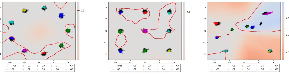
This is illustrated in Figure 5. The left two figures show thesamebest response byC: zoomed in on the data and zoomed out to cover some fake outliers. Clearly,Cneeds to find creative solutions to try and both remove the faraway points and also do good near the real data. As a result, it ends up with the shown narrow beams in an effort to give high score to the true data points (a very broad beam would lower their scores), but this exposesCto being exploited in later iterations:G needs to merely shift the samples to some other part of the vast empty space around the data.
This phenomenon is nicely illustrated by the remaining three plots (that are from a different training run, but illustrate it well): the middle plot shows an NE that targets one beam, this is exploited byGin its next best response (fourth image, note the different scales on the axes, the ‘beam’ is the same). The process continues, andCwill need to find mixtures of all these type of complex counter measures (rightmost plot). This process can take a long time.
PNM with added uniform fake data. The GANG formalism allows us to incorporate a simple way to resolve this issue and make training more effective. In each iteration, we look at the total span (i.e., bounding box) of the real and fake data combined, and we add some uniformly sampled fake data in this bounded box (we used the same amount as fake data produced byG). In that way, we further guideCin order to better guide the generator (by directly making clear that all the area beyond the true data is fake). The impact of this procedure is illustrated by Figure 6, which shows the payoffs that the maintained mixturesµG, µCachieve against the RBBRs computed against them (so this is a measure of security), as well as
the ‘payoff for tests’ (uBR). Clearly, adding uniform fake data leads to much faster convergence. As such, we perform our
main comparison to GANs with this uniform fake data component added in.
B.2. A measure of exploitability
[image:14.612.71.514.213.303.2]Figure 6: Convergence without (left) and with (right) adding uniform fake data. Shown is payoff as a function of the number of iterations of PNM: generator (blue), classifier (green), tests (red). The tests that do not generate positive payoff (red line <0) are not added to the mixture.
Here we propose a measure to test how far from a Nash equilibrium we might be by measuring to what extent the found solution is exploitable by adversaries of some complexity. While this is far from a perfect measure, ourselves only being equipped with bounded computational resources, this might be the best we can do.
In particular, recall that at an NE, we realize the value of the game:
min µC
max µG
uG(µG, µC) = max µG
min µC
uG(µG, µC) =v∗ (4)
In other words, for an equilibriumhµ∗G, µ∗Ciwe have that:
max µG
uG(µG, µ∗C) =v
∗ (5)
min µC
uG(µ∗G, µC) =v∗= min µC
−uC(µ∗G, µC) =−max µC
uC(µ∗G, µC) (6)
which means thatmaxµCuC(µ
∗
G, µC) =−v∗. It also means that if we would knowv∗, we would be able to say ‘how far
away’ some foundµ˜Cis from an equilibrium strategyµ∗C(in terms of value) by looking at thebest-response exploitability:
explBR( ˜µC) = max µG
uG(µG,µ˜C)−v∗≥0 (7)
where the inequality holds assuming we can find the actual best response. Similarly for aµ˜Gwe can have a look at
min µC
uG( ˜µG, µC)−v∗≤0
I.e., ifµ˜Gis an equilibrium strategyminµCuG( ˜µG, µC) =v
∗but ifµ˜
Gis less robust, the minimum is going to be lower
leading to a negative value of the expression (again assuming perfect best responseµC). Since negative numbers are
unnatural to interpret as a distance, we define (again, assuming perfect best response computation):
explBR( ˜µG) =v∗−min µC
uG( ˜µG, µC) =v∗+ max µC
−uG( ˜µG, µC) =v∗+ max µC
uC( ˜µG, µC)
| {z }
at least−v∗
≥0 (8)
Note that, expanding the payoff function, and realizing that the maximum will be attained at a deterministic strategysC:
explBR( ˜µG) =v∗+ max sC
Ex∼pd[φ(sC(x))] +Ez∼pz,z∼µ˜G(z)[φ(1−sC(x))]
| {z }
‘training divergence or metric’
which means this exploitability corresponds “to optimizing the divergence and distance metrics that were used to train the GANs” (Im et al., 2018), offset byv∗.
In the theoretical non-parametric setting (with infinite capacity densities as the strategies) this is directly useful, because then we know that the generator is able to exactly match the density, and thatv∗= log 4(for thelogmeasuring function, which leads to a correspondence to the Jensen-Shannon divergence (Goodfellow et al., 2014)), sinceCwill not be able to discriminate (give higher ‘realness score’ to) real data from on fake data.
However, this may not be a score that is attainable in finite GANG or GANs: First, there might not be a (mixture of) neural networks in the considered class that will match the data density, second there might not be classifier strategies that perfectly classify this discrepancy between the true and generated fake data. Which means that we can not deducev∗. Therefore, even when we assume we can compute perfect best responses, in the finite setting computing these distances might not be sufficient to determine how far from a Nash equilibrium we are. Like Im et al. (2018) and others before them, one might hope that using a neural network classifier to compute a finite approximation to the aforementioned divergences and metrics., i.e., approximatingexplBR( ˜µ
G), will still give a way to compare generators (and it does), but it does not tell how far from
equilibrium one is.
However, even though we do not knowv∗,in the case where we can compute perfect best responses, we can compute a notion of distance of a tuplehµ˜G,µ˜Cito equilibrium by looking at the sum:
explBR( ˜µG,µ˜C),explBR( ˜µC) +explBR( ˜µG) =
max µG
uG(µG,µ˜C)−v∗
+
v∗+ max µC
uC( ˜µG, µC)
= max µG
uG(µG,µ˜C) + max µC
uC( ˜µG, µC) (9)
So by reasoning about the tuple( ˜µG,µ˜C)rather than onlyµ˜G, we are able to eliminate the factor of uncertainty:v∗.
We therefore propose to take this approach, also in the case where we cannot guarantee computing best responses (the second factor of uncertainty). However, note that in (9), since both terms are guaranteed to be larger than 0, we do not need to worry about cancellations of terms and the measure will never underestimate. This is no longer the case when using approximate maximization. Still we can define aresource-boundedvariant:
explRB( ˜µG,µ˜C) , (RBmaxµGuG(µG,µ˜C)−v
∗) + (v∗+RBmax
µCuC( ˜µG, µC)) (10)
= RBmaxµGuG(µG,µ˜C) +RBmaxµCuC( ˜µG, µC). (11)
It does not eliminate the second source of uncertainty, but neither does approximatingexplBR( ˜µ
G). This is a perfectly
useful tool (a lower bound to be precise) to get some information about the distance to an equilibrium, as long as we are careful with its interpretation. In particular, since either or both of the terms of (10) could end up being lower than 0 (due to failure of computing an exact best response), we might end up underestimating the distance, and we can even get negative values. However,explRBis still useful forcomparingdifferent found solution pairshµ˜
G,µ˜Ciandµ˜G0,µ˜C0as
long as we use the same computational resources to compute approximate best responses against them. Negative values of explRB( ˜µ
G,µ˜C)should be interpreted as “robust up to our computational resources to attack it”.
C. Additional empirical results
C.1. Low generator learning rate
Figure 7 shows the results of a lower learning rate for the generator for all 9 mode tasks. The general picture is the same as for the random 9 modes task treated in the main paper: the modes are better covered by fake data, but in places we see that this is at the expense of accuracy.
C.2. Exploitability results
Figure 7: Results for PNM with a learning rate of7−4for the generator. Compare with the first row of Figure 2.
distinguishes real and generated samples, and the classifier tries to determine which generator a sample comes from. Similar to Goodfellow et al. (2014), MGAN presents a theoretical analysis assuming infinite capacity densities. We use MGAN as a state-of-the art baseline that was explicitly designed to overcome the problem of mode collapse.
Figure 8 shows the results of MGAN on the mixture of Gaussian tasks. MGAN results were obtained with an architecture and hyperparameters which exactly match those proposed by Hoang et al. (2018) for a similar task. This means that the MGAN models shown use many more parameters (approx. 310,000) than the GAN and GANG models (approx. 2,000). MGAN requires the number of generators to be chosen upfront as a hyperparameter of the method. We chose this to be equal to the number of mixture components, so that MGAN could cover all modes with one generator per mode. We note that PNM does not require such a hyperparameter to be set, nor does PNM require the related “diversity” hyperparameter of the MGAN method (calledβin the MGAN paper).
[image:17.612.63.540.448.570.2]Looking at Figure 8, we see that MGAN results do seem qualitatively quite good, even though there is one missed mode (and thus also one mode covered by 2 generators) on the randomly located components task (right column).
Figure 8: Results for MGAN on several mixture of Gaussian tasks with 9 modes. Markers correspond to samples created by each generator.
Figure 9 shows our exploitability results for all three tasks with nine modes. We observe roughly the same trend across the three tasks. The left column plots show the exploitability of GANG after different numbers of iterations (with respect to an attacker of fixed complexity: 453 parameters for the attacking G and C together), as well as the number of parameters used in the solutions found in those iterations (a sum over all the networks in the support of the mixture for both players). Error bars indicate standard deviations over 15 trials. Note how the exploitability of the found solution monotonically decreases as the PNM iterations increase.
Figure 9: Exploitability results all 9 mode tasks. Top to bottom: round, grid, random.
shown in the left column, but repositioned at the appropriate place on the x-axis. All data points are exploitability of models that were trained until convergence. Note that here the x-axis shows the complexity in terms of total parameters. The figure shows an approximately monotonic decrease in exploitability for GANGs, while GANs and MGANs with higher complexity are still very exploitable in many cases. In contrast to GANGs, more complex architectures for GANs or MGANs are thus not necessarily a way to guarantee a better solution.
Additionally, we investigate the exploitability of the trained models presented in Figure 1 when attacked by neural networks of varying complexity. These results are shown in the right column of Figure 9. Clearly shown is that the PNM-GANG is robust with near-zero exploitability even when attacked with high-complexity attackers. The MGAN models also have low exploitability, but recall that these models aremuchmore complex (GANG and GAN models have approximately 2,000 parameters, while the MGAN model involves approximately 310,000 parameters). Even with such a complex model, in the ‘random’ task, the MGAN solution has a non-zero level of exploitability, roughly constant for several attacker complexities.
This is related to the missed mode and the fact that two of the MGAN generators collapsed to the same lower-right mode in Figure 1. In stark contrast to both PNM-GANGs and MGAN, we see that the converged GAN solution is exploitable already for low-complexity attackers, again suggesting that the GAN was stuck in an Local Nash Equilibrium far away from a (global) Nash Equilibrium.
As stated in the main paper, the variance of the exploitability depends critically on the solution that is attacked. The top row of Figure 10 shows the results of three different attacks of theGagainst theµCfound by the GAN (top), and PNM-GANG
(bottom). We see that in the top row, due to the shape ofµC, the attacking generators reliably find the blue region with large
classifier scores. On the other hand, in the bottom row, we see that the attacking generators sometimes succeed in finding a blue area, but sometimes get stuck in a local optimum (bottom left plot).
Figure 10: Found best response generators against a fixed GAN (top) and PNM-GANG (bottom) classifier.
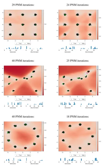
D. Interleaved training for faster convergence
In order to speed up convergence of PNM-GANG, it is possible to train best responses ofGandCin parallel, givingG access to the intermediate results offRBBR
C . The resulting algorithm is shown in Algorithm 2.
In this case, the loss with whichGis trained depends not only on the scores given by the current mixture of classifiers,µC,
but also on the classification scores given byC. Formally, the new proposed loss forGis a weighted sum of the losses if it were to be evaluated againstµCandC, respectively. Clearly, the best response computation presented in the paper
corresponds to the case in which the weight of the loss coming fromCis zero. Intuitively, this gives the generator player the chance to be one-step ahead of the discriminator in discovering modes that are not being currently covered byµG.
This technique may interfere with the convergence guarantees provided above. It might not be the case that we are in fact computing a resource-bounded best-response forGanymore. However, in practice it performs very well: it reduces the
Algorithm 2INTERLEAVEDTRAININGPNMFORGANGS
1: hsG, sCi ←INITIALSTRATEGIES()
2: hµG, µCi ← h{sG},{sC}i .set initial mixtures
3: whileTruedo
4: whileTrainingdo
5: sC←GRADIENTSTEPC(µG)
6: sG←GRADIENTSTEPG(µC, sC)
7: end while
8: // Expected payoffs of these ‘tests’ against mixture: 9: uBRs←uG(sG, µC) +uC(µG, sC)
10: ifuBRs≤0then
11: break
12: end if
13: SG←AUGMENTGAME(SG, sG, sC)
14: hµG, µCi ←SOLVEGAME(SG)
15: end while
Normal best responses Interleaved training
29 PNM iterations: 24 PNM iterations:
40 PNM iterations: 25 PNM iterations:
[image:21.612.128.476.91.650.2]40 PNM iterations: 18 PNM iterations: