arithmetic
.
White Rose Research Online URL for this paper:
http://eprints.whiterose.ac.uk/3762/
Article:
Gamito, M.N. and Maddock, S.C. (2007) Ray casting implicit fractal surfaces with reduced
affine arithmetic. The Visual Computer, 23 (3). pp. 155-165. ISSN 1432-2315
https://doi.org/10.1007/s00371-006-0090-7
[email protected] https://eprints.whiterose.ac.uk/ Reuse
Unless indicated otherwise, fulltext items are protected by copyright with all rights reserved. The copyright exception in section 29 of the Copyright, Designs and Patents Act 1988 allows the making of a single copy solely for the purpose of non-commercial research or private study within the limits of fair dealing. The publisher or other rights-holder may allow further reproduction and re-use of this version - refer to the White Rose Research Online record for this item. Where records identify the publisher as the copyright holder, users can verify any specific terms of use on the publisher’s website.
Takedown
If you consider content in White Rose Research Online to be in breach of UK law, please notify us by
The Visual Computer 23(3):155–165 (March 2007)
Online corrected version athttp://www.dcs.shef.ac.uk/~mag/raycast.html
Manuel N. Gamito · Steve C. Maddock
Ray Casting Implicit Fractal Surfaces
with Reduced Affine Arithmetic
Abstract A method is presented for ray casting implicit
sur-faces defined by fractal combinations of procedural noise functions. The method is robust and uses affine arithmetic to bound the variation of the implicit function along a ray. The method is also efficient due to a modification in the af-fine arithmetic representation that introduces a condensation step at the end of every affine arithmetic operation. We show that our method is able to retain the tight estimation capab-ilities of affine arithmetic for ray casting implicit surfaces made from procedural noise functions while being faster to compute and more efficient to store.
Keywords Affine arithmetic·Implicit Surfaces· Proced-ural Noise Functions·Ray Casting
1 Introduction
This work develops an algorithm for ray casting implicit fractal surfaces generated from procedural noise functions. An implicit surface is defined as the set of all points for which the evaluation of some continuous function f :R3→ Rgives zero. If the function f is a fractal with dimension Df, the implicit surface, being a zeroset of this function, is
also fractal with dimension Df−1 [29]. A common
proced-ural technique to obtain functions that are fractal over a finite range of scales is to accumulate several layers of noise. Each The first author is supported by grant SFRH/BD/16249/2004 from Fundac¸˜ao para a Ciˆencia e a Tecnologia, Portugal.
Manuel N. Gamito
Department of Computer Science The University of Sheffield 211 Portobello Street Sheffield S1 4DP
E-mail: [email protected] Steve C. Maddock
Department of Computer Science The University of Sheffield 211 Portobello Street Sheffield S1 4DP
E-mail: [email protected]
layer consists of a scaled and frequency shifted copy of some original band-limited procedural noise function n [25].
Implicit fractal surfaces are one example of
hypertex-tures [24]. Hypertexhypertex-tures use functions to add volumetric
de-tail to the surface of objects, thereby increasing their visual complexity. Hypertextured objects can either be visualised with a volume rendering approach or converted to an impli-cit surface representation [10].
Another application for implicit fractal surfaces is in
pro-cedural planet modelling [19]. One seeks to describe the
ter-rain of an entire planet by perturbing the surface of a sphere with an appropriate fractal function. If the terrain is to be realistic, however, the implicit surface cannot be allowed to split into separate disconnected pieces. This possibility is currently avoided with the use of procedural noise functions in the form n(x/kxk), effectively turning the implicit surface into a procedural displacement map over the sphere.
pro-posed by de Cusatis Jr. et al., is less efficient than the IA implementation of Mitchell for ray casting implicit surfaces generated from fractal sums of procedural noise functions. This has motivated our use of a reduced representation for AA, which is just as accurate as the original one while being more efficient [15]. It is the use of this reduced AA repres-entation for ray casting implicit surfaces based on procedural noise functions that is the focus of this paper.
Section 2 presents previous work in this area. Section 3 gives a general formulation for procedural noise and applies this formulation to three commonly used noise functions. Understanding how noise functions are procedurally eval-uated is essential to understanding why the reduced AA rep-resentation works. Section 4 presents affine arithmetic and explains how it is used to solve the ray-surface intersec-tion problem of ray casting. The reduced AA framework is then presented and shown to be a simple modification of the standard AA framework. Section 5 shows results and presents a comparison between reduced AA, standard AA and IA. Section 6 presents conclusions, suggests possible enhancements, and shows other areas where our technique can be successfully applied.
2 Previous Work
Many methods have been presented to solve the intersection problem between a ray and an implicit surface. We concen-trate here on methods that are robust. These methods can al-ways find the correct intersection point and are limited only by the floating point precision of the machine. A survey of such methods is given by Hart [8].
Robust implicit surface intersection methods were ini-tially developed for surfaces with a simple and well known shape. If the function f(x)is a polynomial then the impli-cit surface is said to be algebraic and the intersection points can be obtained with polynomial root finders [7]. Surfaces generated by sweeping a sphere along a curve, called
gener-alised cylinders, and surfaces that are subject to non-linear
deformations have also been considered [30, 1].
Implicit surfaces based on the blending of compactly supported radial basis functions are popular because of their ability to model objects with complex topology. Many au-thors who have worked with this type of surface have also developed ray intersection algorithms for them. Such au-thors include Blinn with his blobby model, Nishimura et al. with metaballs and Wyvill and Trotmann with soft
ob-jects [2, 20, 33]. Sherstiuk has developed a general
intersec-tion method for surfaces generated from sums of compactly supported basis functions [26]. His method approximates any basis function with piecewise Hermite polynomials, the roots of which can then be found with analytical formulas.
Two general approaches can be followed to find the in-tersection between a ray and an implicit surface when the function f that generates the surface has an arbitrary shape. One approach is based on Lipchitz bounds and the other is based on interval arithmetic. Lipchitz bounds impose a limit
on the maximum rate of change that f can take inside some region of space. Kalra and Barr successfully rendered
LG-surfaces by advancing rays inside an octree structure [12].
Inside each cell of the octree, a Lipchitz bound L is used for
f and another Lipchitz bound G is used for the derivative
of f along the ray direction. Hart also uses Lipchitz bounds in his sphere tracing method [9]. Unlike Kalra and Barr, it is not necessary to employ Lipchitz bounds for the derivat-ives of f . The method works by marching along a ray with steps that are guaranteed not to cause intersection with the surface. In both the LG-surface method and in sphere tracing it is necessary to specify a priori Lipchitz bounds related to the function f that one wishes to use. That can be difficult in a general case although Kalra and Barr and also Hart present bounds for some commonly used functions. If the Lipchitz bounds are not optimal, these methods will converge more slowly.
Worley and Hart introduced several optimisations in the sphere tracing method for the case of implicit surfaces gen-erated from hypertextures [32]. The improved sphere tracing method takes into account the fact that hypertextured objects are often generated from the sums of many procedural func-tions. Other optimisations include a spatial coherence tech-nique to reduce the number of function evaluations and im-age coherence and overshooting techniques to increase the stepping size along the rays.
Mitchell computes ray-surface intersections with inter-val arithmetic [16]. Interinter-val arithmetic (IA) is a framework that replaces arithmetic operators and function evaluations on real numbers with equivalent operators and functions that are evaluated on intervals [17]. With IA it is possible to ob-tain interval bounds for the variation of f along some arbit-rary span along a ray. The method by Mitchell performs a recursive binary subdivision along the length of a ray, com-puting interval bounds for the function and its derivative in-side each ray span. Newton’s method is used to find the root once the interval bounds indicate the function has become monotonic inside some ray span. The method by Mitchell was later extended to use affine arithmetic (AA), instead of IA [4]. Ray casting with AA produces interval bounds that are much tighter than those obtained with IA, therefore in-creasing the efficiency of the intersection algorithm. One ad-vantage of interval methods over Lipchitz methods is that interval bounds are computed automatically and on the fly. It is not necessary to supply some initial parameter, in the form of a conservative estimate for the Lipchitz bound, that will ultimately determine the efficiency of the algorithm.
3 Procedural Evaluation of Noise Functions
dy-Ray Casting Implicit Fractal Surfaces 157
namic phenomena such as fire, water or clouds [5]. The key to the success of procedural noise functions is that they can be evaluated independently at any desired point in space.
The value of a procedural noise function n at some point
x inR3depends on the position of x relative to a discrete but
infinite set S={xi∈R3: i=0,1,2, . . .}of node points xi
that are distributed throughout space. Because S has an infin-ite number of node points, the evaluation of n(x)is feasible when n(x)is made to depend only on a small subset S(x)
of S. At each location x, the subset S(x)is the finite set of node points in S that surround x according to some specified criterion.
For our purposes, we can define the value of a procedural noise function n at x as a sum of kernel functions φk that
depend on the displacement vectors between x and the node points in S(x):
n(x) =
L
∑
k=0φk(d0,d1, . . . ,dN), (1)
where dj=x−xj and xj, with j=0,1, . . . ,N, belongs to
S(x). The characteristics of each particular noise function come from the choice of several factors, namely:
– The shape of the kernels. – The number L of kernels used. – The criterion used to define S(x).
– The distribution of the xiin space to form S.
The random fluctuations exhibited by procedural noise result from the introduction of stochastic components into some of the previous factors. In some cases of procedural noise functions, the distribution of node points through space follows a desired probability density. Random variables are also often included in the definition of the kernel functions.
3.1 Perlin Gradient Noise Functions
Perlin’s gradient noise function was the first procedural noise function to be proposed in the literature [22]. In this noise function, the node points xi coincide with the vertices of
a regular lattice placed at integer coordinate positions: S=
{(u,v,w): u,v,w∈Z}. For each location x, the set S(x)is
made of the eight node points at the vertices of the lattice cell in which x resides. There are eight kernels and each one depends on a single node point from S(x). A kernelφ that depends on the displacement dj= (xj,yj,zj), relative to
node point xj, is written as:
φ(dj) = (ξ1xj+ξ2yj+ξ3zj)h(xj)h(yj)h(zj). (2)
The function h is a cubic hermite polynomial and the vector (ξ1,ξ2,ξ3) is randomly distributed over the surface
of a sphere with unit radius. There are several variations of Perlin’s gradient noise function, which include Perlin’s value noise function and value-gradient noise function, but these will not be described here [21]. They fit easily into for-mulation (1) with kernels that are similar to (2). Recently,
Perlin improved his gradient noise function by using quintic hermite polynomials for h and having(ξ1,ξ2,ξ3)be a
ran-dom vector that can only take values from a discrete set of vectors [23].
3.2 Sparse Convolution Functions
Sparse convolution noise functions were first proposed by Lewis [13]. As with Perlin’s noise functions, a regular lat-tice placed at integer positions is also used. Inside each cell in this lattice, K node points are uniformly distributed. This simple scheme attempts to approximate a Poisson distribu-tion of node points. The value of n at each locadistribu-tion x de-pends on the node points of the cell that contains x plus the node points in the twenty six surrounding cells. The set
S(x), therefore, always contains 27K node points. There is an equal number of kernels, one for each node point. A ker-nelφdepends only on the distancekdjkto its corresponding
node point:
φ(dj) =ξh(kdjk). (3)
The scalarξis a gaussian random variable and the func-tion h can take any shape as long as it is compactly suppor-ted on the interval[0,1]. This last requirement is necessary to guarantee that only the 27K node points in the cell that contains x and in its immediate neighbours can possibly in-fluence the value of n(x).
Sparse convolution noise functions are more expensive to evaluate than gradient noise functions. A total of 27K kernels need to be evaluated against only eight for Perlin’s gradient noise function. Sparse convolution functions, how-ever, have the advantage of providing exact control over the frequency spectrum of the resulting noise. It is possible to show that the spectrum of n for sparse convolution noise functions is proportional to the spectrum of the function h that is chosen for (3) [13].
3.3 Cellular Texture Functions
Cellular texture functions, proposed by Worley, rely on a Voronoi decomposition of space based on the location of the
xi node points [31]. As with sparse convolution functions,
an approximation to a Poisson distribution of node points is generated inside an integer lattice, although the technique used to achieve this effect is slightly different from the one employed by Lewis. The kernels for cellular texture noise functions consist of the ordered set of increasing distances between any location x and the node points. For some loc-ation x, let D(x) ={kdik: i=0,1,2. . .}be the set of
dis-tances from x to all node points in S. Let also p :N0→N0
be a permutation of the indices in D(x)so that the new set
D(x) ={kdjk: j=p(i),i=0,1,2. . .}is ordered by
increas-ing distances. The j-th kernel function is then taken as the
j-th element in the ordered set D(x):
where ajis some chosen scaling constant. Worley points out
that only the kernel functionsφ0toφ3are useful for texture
synthesis. Theφjwith j>3 resembleφ3and do not add
sig-nificant new details. With the first four kernel functions, sev-eral interesting combinations are possible by choosing the appropriate values of the aj constants. Kernel functions can
also be turned off by setting aj=0.
The technique Worley employs to distribute the node points throughout the integer lattice guarantees that for every location x the four nearest node points will always be found inside the lattice cell that contains x or inside one of its neighbours. Similarly to sparse convolution noise functions, the set S(x), used to computeφ0toφ3, is then made of all
the node points that are contained inside the 3×3×3 cube of lattice cells that is centred on the cell containing x.
4 Robust Ray Casting of Implicit Surfaces
Ray casting an implicit surface consists of determining the intersection point between the surface and any ray, paramet-erised as r(t) =o+tl with t>0. Because the implicit sur-face is the zeroset of some function f , ray casting amounts to finding the first root of the non-linear equation:
f(r(t)) =0. (5)
Let the parameter along the ray vary inside some inter-val T= [tmin,tmax]. For simplicity of notation, let us also
in-troduce the auxiliary function g= f◦r. We wish to find an
interval estimate G(T)of the corresponding variation in g(t)
as t takes values from T . The function G is called an
inter-val extension of g. The interinter-val extension function provides
information about the presence of roots of (5) inside some interval. If 06∈G(T)then no root can be present in T . If, on the other hand, 0∈G(T), a root may or may not exist in T . This is because current techniques for computing G can only provide a conservative interval estimate that con-tains the true variation of g. The fact that 0∈G(T)does not necessarily mean that g(t) =0 for some t∈T . The best
strategy in this case is to split T into smaller intervals and test the interval extension function on each of them.
Figure 1 lists a robust algorithm, calledRayIntersect, that is used to find the first intersection point between a ray and the implicit surface. The algorithm relies on the subdi-vision of an initial interval T0and the information returned
by the interval extension function G. A stack is used to store the subdivided intervals that are waiting to be tested for the existence of roots. The algorithm terminates either when a small enough interval bounding a root has been found or when the stack becomes empty. The latter scenario occurs in situations where a ray does not intersect the surface. Each interval taken from the stack is subdivided if there is the pos-sibility that it may contain a root. The order with which the two subintervals are then pushed onto the stack is not arbit-rary. By pushing Trfirst and then Tl, the nearest intersection
is guaranteed to be found.
push T0onto stack;
while stack not empty
pop T= [tmin,tmax]from the stack;
if 0∈G(T)
if tmax−tmin<ε return tmin; let ti= (tmax+tmin)/2; let Tl= [tmin,ti]; let Tr= [ti,tmax]; push Tronto stack; push Tlonto stack;
Fig. 1 TheRayIntersectalgorithm.
TheRayIntersectalgorithm is a simplified version of the interval algorithm by Mitchell [16]. In Mitchell’s ori-ginal algorithm, an interval extension G′of the derivative of
g along the ray was also computed. When 0∈G(T)and 06∈
G′(T) were both verified, the function was known to have an isolated root inside the interval T and Newton’s method could then be used to provide quadratic convergence. In the case of fractal combinations of procedural noise functions, however, g varies erratically and only for very small inter-vals do the conditions for monoticity exist that enable us to isolate a single root. We have found that the use of G′does not provide any speedup while ray casting fractal implicit surfaces and, in fact, slows down the algorithm since two interval extensions have to be computed instead of one. de Cusatis Jr. et al. reached the same conclusion for the type of implicit surfaces that they were interested in rendering [4].
4.1 Standard Affine Arithmetic
Affine arithmetic is a technique proposed by de Figueiredo and Stolfi [6]. This technique can provide accurate estim-ates for the interval extension function G(T)featured in the
RayIntersect algorithm. Affine arithmetic represents an improvement over the previous interval arithmetic technique [17]. The representation of some quantity with affine arith-metic (AA) tries to model the uncertainties about that quant-ity so that it is always bounded inside a known interval. The advantage over the simpler interval arithmetic framework is that AA tries to keep correlations between quantities, cal-culated along some arbitrarily long chain of computations. AA keeps correlations between similar quantities through the use of error symbols. A quantity ˆt in AA is represen-ted as a central value t0plus a sequence of error symbols ei,
each with its associated error coefficient ti:
ˆt=t0+t1e1+t2e2+· · ·+tnen. (6)
The error symbols lie in the interval[−1,+1]but are oth-erwise unknown and the coefficients tiexpress the
Ray Casting Implicit Fractal Surfaces 159
The computation of affine operations on AA quantities does not result in the creation of any new error symbols1. For two AA quantities ˆu, ˆv and a scalarα, the affine operations are:
αuˆ= (αu0) + (αu1)e1+· · ·+ (αun)en,
ˆ
u±α= (u0±α) +u1e1+· · ·+unen,
ˆ
u±vˆ= (u0±v0) + (u1±v1)e1+· · ·+ (un±vn)en.
(7)
For non-affine operations, like multiplication or square root, a new error symbol must be introduced to express the non-linearity of the operator. The result of some non-affine operator is a new AA quantity ˆw=w0+w1e1+· · ·+wnen+
wkek, where the extra error symbol ekhas been added to the
representation. For example, if ˆw=u ˆˆv, the coefficients of ˆw
are given by:
w0=u0v0,
wi=u0vi+v0ui, for i=1, . . . ,n,
wk=
n
∑
i=1|ui| · n
∑
i=1|vi|.
(8)
The coefficient wk in (8), associated with the newly
in-serted error symbol ek, is positive and represents the
mag-nitude of the error introduced by the linearisation of ˆu ˆv into
an affine form. The same property of wkholds in the case of
all the other non-affine operations.
As a sequence of AA operations progresses, quantities have an increasingly larger number of error symbols, slow-ing down subsequent AA computations and increasslow-ing the memory requirements. This is because, if the uncertainty as-sociated with some error symbol ei of an AA quantity is
not shared with any other AA quantities, the latter must all have a null coefficient for ei. When implementing AA,
cum-bersome book-keeping routines are required to manage the large but sparse sequences of error coefficients2. This ineffi-ciency associated with AA representations has been acknow-ledged by Stolfi and de Figueiredo [27]. They recommend that a procedure called condensation be periodically applied on an AA quantity when its sequence of error symbols grows too large. An AA quantity ˆu, with m error symbols, can be
condensed to form another quantity ˆv, with n<m error
sym-bols, according to:
vi=ui, for i=0, . . . ,n−1,
vn= m
∑
i=n|ui|.
(9)
Condensation brings some large AA quantity ˆu down
to a more manageable size but it also destroys the correla-tion informacorrela-tion that was kept in the error symbols ei, with
1 Assuming that rounding errors are ignored. Otherwise, affine
oper-ations, just like their non-affine counterparts, require the insertion of a new error symbol that accounts for the rounding error of the operation.
2 A simpler alternative would be to store in full all the coefficients
of an AA quantity. This would be wasteful of memory, considering that many of those coefficients are zero. It would also be wasteful of CPU cycles. As example (8) shows, the computation of AA operations involves a loop over all the eierror symbols. If the sequence of
coeffi-cients is sparse, many of the loop iterations become unnecessary.
n<i6m. This is not a problem if the aforementioned error
symbols were unique to ˆu. The accuracy of subsequent
com-putations is affected, however, if the ei were being shared
with other AA quantities that are involved in those compu-tations.
4.2 Reduced Affine Arithmetic
The problem of having to deal with ever increasing sets of error symbols in standard AA has motivated our use of a re-duced AA form for ray casting implicit surfaces made from procedural noise functions. Reduced affine arithmetic was proposed by Messine as the first of several possible sions to affine arithmetic [15]. In his work, this first exten-sion is called Affine Form 1 (AF1).
As equation (1) shows, procedural noise functions are built from sums of independent kernel functions. No correl-ations exist between the sequence of computcorrel-ations that are performed for any two kernel functionsφiandφjduring the
computation of n. Correlations during the evaluation of a procedural noise function have a very localised nature and are isolated inside the sequence of computations for each individual kernel. The only global correlation that is expec-ted to exist throughout the computation of n is relaexpec-ted to the uncertainty with the position of the root t along a ray. This happens when n is embedded in the equation g(t) =0 that must be solved by the ray caster.
Our reduced AA representation ˆt is equivalent to an AF1 representation which considers only two error symbols: the symbol e1, expressing the uncertainty along the ray, and the
symbol e2, which is always non-negative and expresses
un-certainties involved in the computation of ˆt alone. The error symbol e1 is the only symbol that is shared between ˆt and
other AA quantities. The expression for ˆt is:
ˆt=t0+t1e1+t2e2. (10)
The starting point for the computation of the interval ex-tension G(T), as part of theRayIntersectalgorithm, is the conversion of the interval T = [tmin,tmax] into the reduced
AA form ˆt:
t0= (tmax+tmin)/2,
t1= (tmax−tmin)/2,
t2=0.
(11)
Reduced AA operations are always followed by a con-densation step to remove any extra error symbols that would have been introduced otherwise. Reduced AA can, therefore, be seen as a modification of affine arithmetic that employs an aggressive form of condensation. We present, as an ex-ample, the case of the multiplication between two reduced AA quantities ˆu and ˆv. Originally, the result of this
multi-plication would give: ˆ
u ˆv=u0v0 + (u0v1+v0u1)e1+
where we have written the second error symbols of ˆu and ˆv
as e2uand e2v, respectively, to make it clear that they are not
correlated. The last three terms of (12) are condensed into a new symbol e2that is unique to the ˆu ˆv quantity, giving:
ˆ
u ˆv=u0v0 + (u0v1+v0u1)e1+
+ |u0|v2 + |v0|u2 + (|u1|+u2)·(|v1|+v2)
e2. (13)
In practice, all operations in reduced AA are modified so that a condensation step is automatically built into them. The affine operators (7) now become:
αuˆ= (αu0) + (αu1)e1+ (|α|u2)e2,
ˆ
u±α= (u0±α) +u1e1+u2e2,
ˆ
u±vˆ= (u0±v0) + (u1±v1)e1+ (u2+v2)e2.
(14)
The last stage in the computation of an interval extension for ray casting is the conversion of the reduced AA form
ˆ
g=g(ˆt)into the interval G(T) = [gmin,gmax], which allows
the test 0∈G(T)to be performed trivially:
gmin=g0− |g1| −g2, gmax=g0+|g1|+g2,
0∈G(T)⇔gmin606gmax.
(15)
An analysis of the localised nature of the correlations during AA computations, as part of the evaluation of a pro-cedural noise function, requires that the kernels for each individual noise function be examined in turn. In the case of Perlin’s gradient noise function, the kernel (2) has three AA multiplications, each of which would introduce new er-ror symbols in a standard AA representation. However, once these three multiplications are performed, the evaluation of
φ(dj)is complete and the new error symbols can be safely
condensed. At the same time, the AA evaluation of the cubic hermite polynomial h is performed through a direct process of Chebyshev affine approximation rather than applying all the usual algebraic operations [27, 11]. This means that no internal correlations have to be considered during the evalu-ation of h because the reduced AA result is computed in one single step. In the end, it is possible to say that the evaluation ofφ(dj)with reduced AA does not lose any correlation
in-formation and has the same accuracy as standard AA. In the case of Lewis’s sparse convolution noise func-tion, the kernel (3) depends only on the distance kdjkto
some node point xj. This distance computation features four
non-affine operations, namely three squares and one square root operation. The distancekdjk, however, is involved in
the computation ofφjalone and does not influence the other
φikernels (with i6= j) that are required for the evaluation of
n. The condensation of the new error symbols from the
eval-uation ofkdjkdoes not, therefore, lead to any loss of
accur-acy. The evaluation of the function h is performed directly by Chebyshev approximation and, again, we can say that a reduced AA computation ofφj is as accurate as a standard
AA computation.
tmin
tmax to
min
[image:7.612.334.513.92.236.2]tmaxo
Fig. 2 The information conveyed by reduced affine arithmetic for the
behaviour of the function g inside an interval T= [tmin,tmax].
In the case of Worley’s cellular texture function, the ker-nel is evaluated by iteratively applying a binary minimum operator min(li,lj)on all the pairs of distances lk=kdkk
from x to the node points that belong to the set S(x). The minimum operator is evaluated with affine arithmetic ac-cording to the expression:
min(li,lj) =
li+lj
2 −
li−lj
2 . (16)
For example, if li>ljwe have min(li,lj) = (li+lj)/2−
(li−lj)/2=lj. This exact cancellation effect can only be
achieved if all correlations between li=kdikand lj=kdjk
are maintained. However, the distance computations with re-duced AA involve the condensation of error symbols, as we have seen in the case of Lewis’s sparse convolution noise function, and an exact cancellation cannot be obtained. For this reason, the application of reduced AA to cellular tex-ture functions incurs a loss of accuracy. In Section 5, the loss of accuracy of reduced AA will be compared against its increased performance relative to standard AA for cellular texture functions.
4.3 Interval Optimisation
The idea of optimising the size of the interval bounding the first root of (5) was initially presented by de Cusatis Jr. et al. [4]. We present it here again in the framework of reduced af-fine arithmetic. When implementing theRayIntersect al-gorithm with affine arithmetic, it is possible to reduce the size of the interval T being tested at the start of each itera-tion, and prior to its subdivision, by taking advantage of the extra information provided by reduced AA.
Figure 2 shows an example of the information conveyed by a reduced AA representation of the function g, evaluated inside some interval T = [tmin,tmax]along the ray, for a
situ-ation where g increases smoothly. The purpose of the ray casting algorithm is to find the point where the graph of g crosses the horizontal axis. The reduced AA representation
Ray Casting Implicit Fractal Surfaces 161
(11), is geometrically equivalent to a parallelogram that en-closes the graph of g for the interval T . The bounding inter-val can be optimised by reducing it to To= [tmino ,to
max]prior
to subdivision. It is clear from the drawing that significant convergence towards the root is achieved with just a single evaluation of g(ˆt)in reduced AA form.
The optimised interval Tois obtained from the reduced AA representations ˆt=t0+t1e1for the interval and g(ˆt) = g0+g1e1+g2e2for the function g in the following way:
tmino =max
t0−
g0 g1
t1− g2 |g1|
t1,tmin
,
tmaxo =min
t0−
g0 g1
t1+ g2 |g1|
t1,tmax
.
(17)
A derivation of these equations is given in Appendix A. To summarise, we show here the steps necessary to com-pute the interval extension G(T)in theRayIntersect al-gorithm of Figure 1, after the interval T has been removed from the stack:
1. Compute the reduced AA variable ˆt from T= [tmin,tmax],
written as (10) and with coefficients given by (11). 2. Compute the reduced AA estimate ˆg=g(ˆt), using
re-duced affine arithmetic operators.
3. Compute the interval extension G(T)from ˆg, using (15).
If, after step 3, it is found than 0∈G(T), the optimised interval To= [tmino ,to
max]is obtained from the initial interval
T , its reduced AA representation ˆt, and the estimate ˆg,
us-ing (17). It is To, rather than T , which is then subdivided and its subintervals pushed back onto the stack for further processing during subsequent iterations of the algorithm3.
5 Results
A hypertextured implicit surface generated by the following function was used to test our reduced affine arithmetic ray casting method:
f(x) =kxk −1+0.6
3
∑
k=02−0.8kn(2k+2x). (18) The term kxk −1 is responsible for giving an overall spherical shape to the surface. The remaining summation on the right of (18) employs a procedural noise function n and represents the hypertexture, being responsible for the gen-eration of all the surface detail. This summation produces a fractal surface with a dimension of 2.2, according to Saupe4 [25].
3 When g
1→0, the enclosing parallelogram in Figure 2 tends
to-ward an axis aligned rectangle. In the limit, no optimisation is possible and the original interval T must be subdivided.
4 To be more precise, a fractal surface with dimension 2.2 would
result if the summation had an infinite number of terms, with k∈Z.
[image:8.612.311.526.114.175.2]As it stands, the function (18) produces a fractal surface only over a limited range of scales.
Table 1 Statistics for Perlin’s gradient noise function.
Avg. Evals. p/ray Time
[image:8.612.311.526.206.266.2]IA 78.40 8m27.5s Standard AA 34.60 36m22.9s Reduced AA 34.60 5m57.1s Reduced AA + Int. Opt. 20.81 3m43.2s
Table 2 Statistics for Lewis’s sparse convolution noise function.
Avg. Evals. p/ray Time
[image:8.612.307.530.295.356.2]IA 48.44 26m31.0s Standard AA 23.25 32m24.7s Reduced AA 23.25 10m47.2s Reduced AA + Int. Opt. 13.46 6m29.3s
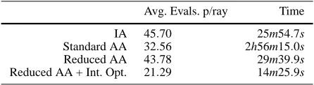
Table 3 Statistics for Worley’s cellular texture function.
Avg. Evals. p/ray Time
IA 45.70 25m54.7s Standard AA 32.56 2h56m15.0s Reduced AA 43.78 29m39.9s Reduced AA + Int. Opt. 21.29 14m25.9s
Figure 3 shows, from left to right, a rendering of the implicit surface when n is Perlin’s improved gradient noise function, Lewis’s sparse convolution function with K=2 (refer to Section 3.2) and Worley’s cellular texture function with a0=1 and a1=a2=a3=0 (refer to Section 3.3). We
have implemented a reduced affine arithmetic model of cel-lular texture functions that can use linear combinations of theφ0andφ1kernels only. We have found that theφ2andφ3
kernels are too complex to implement when using AA. This is due to the difficulty in determining the third and fourth smallest distances in the set S(x)when all thekdjkhave an
arbitrary degree of uncertainty. For this reason, our current implementation of Worley’s cellular texture functions must enforce the restriction a2=a3=0.
Tables 1, 2 and 3 show some statistics that enable a com-parison between all the interval estimation techniques for the procedural noise functions under consideration. We have compared the performance of interval arithmetic (IA), stand-ard AA, reduced AA and reduced AA with interval optim-isation. The rendering time was obtained for a 800×600 resolution image on a dual Athlon 2.1GHz processor. The average number of function evaluations per ray tells how of-ten an interval exof-tension G(T)had to be computed as part of theRayIntersectalgorithm. This statistic is a measure of the accuracy of each particular interval estimation technique. A more accurate technique causes the ray casting algorithm to converge to the intersection point with fewer iterations and fewer interval extension computations.
Fig. 3 An implicit surface representing a sphere that has been hypertextured with three layers of (from left to right) Perlin’s gradient noise
function, Lewis’s sparse convolution noise function and Worley’s cellular texture function.
algorithms. Straightforward replacement of the IA opera-tions with AA equivalents leads to a more inefficient al-gorithm, due to the need to compute sequences of error sym-bol coefficients that grow progressively larger. Nevertheless, standard AA is able to reduce the average number of func-tion evaluafunc-tions, which shows that AA does have the poten-tial to optimise ray-surface intersection algorithms, if only it can be implemented in a more efficient manner.
The better performance of IA over standard AA for the evaluation of procedural noise functions was acknowledged implicitly by Heidrich et al. [11]. In their work, IA was used for computing the interval estimates of a Perlin noise func-tion. These interval estimates were then converted into AA form for use in the rest of the application. The authors do not state a reason for preferring IA over AA when comput-ing a Perlin noise function but it is symptomatic that such a decision was taken in a paper whose purpose was to propose AA as a better alternative to IA.
Efficiency with AA is obtained in the reduced AA rep-resentation. As we had predicted in Section 4.2, no accuracy is lost by the use of reduced AA for the gradient noise func-tion and the sparse convolufunc-tion funcfunc-tion. There is a loss of accuracy in the case of the cellular texture function, which is compensated by its increased computation speed so that, overall, reduced AA performs much better than standard AA for all three procedural noise functions. The final improve-ment comes from optimising the size of the intervals, as ex-plained in Section 4.3. Reduced AA combined with interval optimisation gives the lowest rendering statistics of all inter-val estimation techniques.
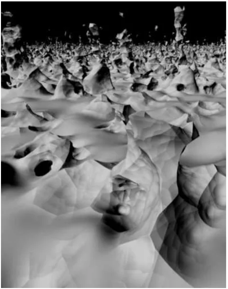
Figure 4 shows a procedurally defined planet. The impli-cit surface uses a combination of the procedural noise func-tions studied in this paper. The faceted aspect of the terrain, in particular, is a consequence of the Voronoi regions created by the cellular texture function. In this example, no attempt was made to avoid the occurrence of disconnected pieces of terrain that arise naturally from the implicit representation, giving the planet a somewhat surrealistic look. This image took 6 hours and 37 minutes to render with reduced AA and
Fig. 4 A procedural planet represented as an implicit surface with a
radius equal to the radius of the Earth and seen from an altitude of 100 metres. The implicit surface uses a mixture of all three procedural noise functions that are studied in this paper.
[image:9.612.302.536.302.599.2]Ray Casting Implicit Fractal Surfaces 163
6 Conclusions and Future Developments
Ray casting implicit fractal surfaces with affine arithmetic becomes efficient only with the introduction of a reduced representation for uncertain quantities. The representation of an uncertain quantity with reduced affine arithmetic uses a maximum of two error symbols. It has been shown that without this reduced representation affine arithmetic would not be able to compete against a simpler interval arithmetic representation. These results were obtained while ray cast-ing implicit surfaces generated from procedural noise func-tions that are widely used in computer graphics. Such pro-cedural noise functions are based on the summation of sev-eral statistically independent terms. By maintaining only the correlation related to the uncertainty in the position of the root along the ray, reduced affine arithmetic can achieve the same results as standard affine arithmetic while being more efficient.
As predicted in Section 4.2 and subsequently confirmed in Section 5, the application of reduced AA to cellular tex-ture functions incurs a loss of accuracy. This is ultimately due to the destruction of important correlation information through the condensation of error symbols. The loss of ac-curacy, however, is compensated by the greatly increased ef-ficiency that comes from dealing with only two error sym-bols for each AA quantity, with a rendering time that drops from almost 3 hours with standard AA to only 29 minutes with reduced AA. It is possible, however, that for some other procedural noise functions, with kernels that we have not tested, the loss of accuracy may be more significant. In such a case, standard AA can be used for the calculation of the kernelφ(d1,d2, . . . ,dn)and a switch to reduced AA can be
done for the remainder of the calculations in (1).
Standard and reduced AA quantities can easily be inter-changed. Any reduced AA quantity is also a valid standard AA quantity that happens to have only two error symbols. The second error symbol e2has to be given a new and unique
index number, after conversion to standard AA, to express the fact that it is not shared with any other standard AA quantities. A standard AA quantity can be transformed to a reduced AA quantity through condensation. For ray casting purposes, it is required that both AA representations agree that the common error symbol e1 is used to express
un-certainty relative to the position of the root along the ray. This is so that the interval optimisation procedure of Sec-tion 4.3 can be properly implemented. In a situaSec-tion like that of Figure 4, where several procedural noise functions are used, the majority of the noise functions would be entirely computed with reduced AA while only the more problem-atic ones would use standard AA internally to compute their kernel functions.
Interpolating implicit surfaces have gained much pop-ularity in recent years because of their ability to interpol-ate any set of constraint points [28, 18]. Interpolating im-plicit surfaces are now the method of choice to generate a continuous and smooth surface approximation from a set of scattered data points. From a structural point of view,
in-terpolating implicit surfaces are entirely similar to sparse convolution noise functions, with equation (1) being used to sum the contribution of several independent radial basis functions (RBFs). Each RBFφ(di)depends only on the
dis-tancekdikto constraint point xi. A RBF is written asφ(di) =
aih(kdik), where h is some continuous and differentiable
function. The difference between this RBF and (3) is only in the meaning of the scaling constant aiorξ, respectively.
The aiare pre-computed so as to cause the surface to
inter-polate through the required constraint points whereas ξ is the outcome of a random variable.
Given the structural similarity between sparse convolu-tion noise funcconvolu-tions and interpolating implicit surfaces made from sums of RBFs we can say that our reduced affine arith-metic method can also be used successfully to render the latter with ray casting. Current methods for rendering inter-polating implicit surfaces resort to sphere tracing, where a Lipchitz bound must be supplied by the user before render-ing takes place [9]. The optimal Lipchitz bound for a con-tinuous and differentiable function f in three dimensions, such as the one generated through (1) for sums of RBFs, is the maximum magnitudek∇fkof the gradient vector. For an arbitrary set of constraint points xi, this maximum gradient
magnitude can only be found through a costly global optim-isation procedure. Morse et al. avoid this procedure by eval-uating k∇fkat a large set of random points and using the maximum value thus obtained as their Lipchitz bound [18]. Clearly, this does not lead to a robust rendering algorithm as it is not possible to guarantee that all correct ray-surface intersections will be found. Problematic areas will be those where the value of f changes more rapidly than predicted by the Lipchitz bound that Morse et al. use. By ray casting inter-polating implicit surfaces with reduced affine arithmetic, one has an automatic, robust, efficient, and verifiable method of computing all ray intersections without the burden of having to estimate the Lipchitz bound as a pre-computation step.
A Derivation of the Interval Optimisation Equation
When computing ˆg=g(ˆt), we have that ˆg=g0+g1e1+g2e2and ˆt= t0+t1e1, where the error symbols e1and e2are unknown but vary in
the interval[−1,+1]. Replacing the expression for ˆt in the expression for ˆg, by way of the e1error symbol, we have:
ˆ
g=g1
t1
(ˆt−t0) +g0+g2e2. (A.1)
Equation (A.1) is the equation for a line in the ˆg-ˆt plane with a
slope of g1/t1. By letting e2vary in[−1,+1]and keeping tmin6ˆt6 tmaxwe sweep the parallelogram that is shown in Figure 2. The upper and lower edges of this parallelogram are obtained from (A.1) when
e2=±1. The intersections of these two edges with the horizontal axis
give the new and optimised limits for the interval. Setting (A.1) equal to zero, with e2=±1, and rearranging, we have:
ˆt=t0− g0 g1
t1± g2 g1
t1. (A.2)
Independently of the sign of g1(g2is always positive and t1is also
left and right solutions to (A.2) along the horizontal axis are, respect-ively:
tmino =t0− g0 g1
t1− g2 |g1|
t1,
tmaxo =t0− g0 g1
t1+ g2 |g1|
t1.
(A.3)
We only use the results from (A.3) if they lead to a tighter interval than the original[tmin,tmax], hence the min and max functions in (17).
Acknowledgements The authors would like to express their gratitude
to Luiz Henrique de Figueiredo for graciously making available the source code used by de Cusatis Jr. et al. [4]. The authors would also like to thank their anonymous reviewers, whose comments helped to improve significantly the clarity of the text.
References
1. Barr, A.H.: Ray tracing deformed surfaces. In: D.C. Evans, R.J. Athay (eds.) Computer Graphics (SIGGRAPH ’86 Proceedings), pp. 287–296. ACM Press (1986)
2. Blinn, J.F.: A generalization of algebraic surface drawing. ACM Transactions on Graphics 1(3), 235–256 (1982)
3. Bloomenthal, J.: Polygonisation of implicit surfaces. Computer Aided Geometric Design 5(4), 341–355 (1988)
4. de Cusatis Jr., A., de Figueiredo, L.H., Gattas, M.: Interval meth-ods for raycasting implicit surfaces with affine arithmetic. In: Proc. XII Brazilian Symposium on Computer Graphics and Im-age Processing (SIBGRAPI ’99), pp. 65–71 (1999)
5. Ebert, D.S., Musgrave, F.K., Peachey, D.R., Perlin, K., Worley, S.P.: Texturing & Modeling: A Procedural Approach, 3rd edn. Morgan Kaufmann Publishers Inc. (2003)
6. de Figueiredo, L.H., Stolfi, J.: Affine arithmetic: Concepts and ap-plications. Numerical Algorithms 37(1–4), 147–158 (2004) 7. Hanrahan, P.: Ray tracing algebraic surfaces. In: P.P. Tanner (ed.)
Computer Graphics (SIGGRAPH ’83 Proceedings), pp. 83–90. ACM Press (1983)
8. Hart, J.: Ray tracing implicit surfaces. In: Modeling, Visualizing and Animating Implicit Surfaces, pp. 13.1–13.15 (1993). SIG-GRAPH ’93 Course Notes 25
9. Hart, J.C.: Sphere tracing: A geometric method for the antialiased ray tracing of implicit surfaces. The Visual Computer 12(9), 527– 545 (1996)
10. Hart, J.C.: Implicit representation of rough surfaces. Computer Graphics Forum 16(2), 91–99 (1997). ISSN 0167-7055
11. Heidrich, W., Slusallek, P., Seidel, H.: Sampling procedural shaders using affine arithmetic. ACM Transactions on Graphics
17(3), 158–176 (1998)
12. Kalra, D., Barr, A.H.: Guaranteed ray intersections with implicit surfaces. In: J. Lane (ed.) Computer Graphics (SIGGRAPH ’89 Proceedings), vol. 23, pp. 297–306. ACM Press (1989)
13. Lewis, J.P.: Algorithms for solid noise synthesis. In: J. Lane (ed.) Computer Graphics (SIGGRAPH ’89 Proceedings), vol. 23, pp. 263–270. ACM Press (1989)
14. Lorensen, W.E., Cline, H.E.: Marching cubes: A high resolution 3D surface construction algorithm. In: M.C. Stone (ed.) Computer Graphics (SIGGRAPH ’87 Proceedings), vol. 21, pp. 163–169. ACM Press (1987)
15. Messine, F.: Extentions to affine arithmetic: Application to un-constrained global optimization. Journal of Universal Computer Science 8(11), 992–1015 (2002)
16. Mitchell, D.P.: Robust ray intersection with interval arithmetic. In: Proceedings of Graphics Interface ’90, pp. 68–74. Canadian Information Processing Society (1990)
17. Moore, R.: Interval Arithmetic. Prentice-Hall (1966)
18. Morse, B.S., Yoo, T.S., Chen, D.T., Rheingans, P., Subramanian, K.R.: Interpolating implicit surfaces from scattered surface data using compactly supported radial basis functions. In: B. Werner (ed.) Proceedings of the International Conference on Shape Mod-eling and Applications (SMI-01), pp. 89–98. IEEE Computer So-ciety (2001)
19. Musgrave, F.K.: Mojoworld: Building procedural planets. In: D.S. Ebert, F.K. Musgrave (eds.) Texturing & Modeling: A Procedural Approach, 3rd edn., chap. 20, pp. 565–615. Morgan Kauffman Publishers Inc. (2003)
20. Nishimura, H., Hirai, M., Kawai, T., Kawata, T., Shirakawa, I., Omura, K.: Object modeling by distribution function and a method of image generation. Trans. IECE Japan, Part D J68-D(4), 718– 725 (1985)
21. Peachey, D.R.: Building procedural textures. In: D.S. Ebert, F.K. Musgrave (eds.) Texturing & Modeling: A Procedural Approach, 3rd edn., chap. 2, pp. 7–94. Morgan Kauffman Publishers Inc. (2003)
22. Perlin, K.: An image synthesizer. In: B.A. Barsky (ed.) Computer Graphics (SIGGRAPH ’85 Proceedings), pp. 287–296. ACM Press (1985)
23. Perlin, K.: Improving noise. ACM Transactions on Graphics (SIG-GRAPH ’02 Proceedings) 21(3), 681–682 (2002)
24. Perlin, K., Hoffert, E.M.: Hypertexture. In: J. Lane (ed.) Computer Graphics (SIGGRAPH ’89 Proceedings), vol. 23, pp. 253–262. ACM Press (1989)
25. Saupe, D.: Point evaluation of multi-variable random fractals. In: H. J¨uergens, D. Saupe (eds.) Visualisierung in Mathematik und Naturissenschaften - Bremer Computergraphik Tage, pp. 114– 126. Springer-Verlag (1989)
26. Sherstyuk, A.: Fast ray tracing of implicit surfaces. Computer Graphics Forum 18(2), 139–147 (1999)
27. Stolfi, J., de Figueiredo, L.H.: Self-validated numerical methods and applications (1997). Course notes for the 21st Brazilian Math-ematics Colloquium
28. Turk, G., O’Brien, J.F.: Modelling with implicit surfaces that in-terpolate. ACM Transactions on Graphics 21(4), 855–873 (2002) 29. Voss, R.F.: Fractals in nature: From characterization to simulation. In: H.O. Peitgen, D. Saupe (eds.) The Science of Fractal Images, chap. 1, pp. 21–70. Springer-Verlag (1988)
30. van Wijk, J.J.: Ray tracing objects defined by sweeping a sphere. Computers & Graphics 9(3), 283–290 (1985)
31. Worley, S.P.: A cellular texture basis function. In: H. Rushmeier (ed.) Computer Graphics (SIGGRAPH ’96 Proceedings), vol. 30, pp. 291–294. ACM Press (1996)
32. Worley, S.P., Hart, J.C.: Hyper-rendering of hyper-textured sur-faces. In: Proc. of Implicit Surfaces ’96, pp. 99–104 (1996) 33. Wyvill, G., Trotman, A.: Ray-tracing soft objects. In: Computer
![Fig. 2 The information conveyed by reduced affine arithmetic for thebehaviour of the function g inside an interval T = [tmin,tmax].](https://thumb-us.123doks.com/thumbv2/123dok_us/8081632.229032/7.612.334.513.92.236/information-conveyed-reduced-afne-arithmetic-thebehaviour-function-interval.webp)