Methods To Reduce Perturbation Effects
In Compressive Sampling
Daniel Heonki Chae
February 2013
For my two daughters, Laura (Minseo) and Olivia (Yunseo), my son Joshua (Joonseo),
Declaration
The work in this thesis is my own except where otherwise stated. It contains no material previously published or written by another person nor material which to a substantial extent has been accepted for the award of any other degree of the university or other institute of higher learning.
Acknowledgements
I thank God for everything, and the Australian government for supporting my study. I also have to thank my supervisors for their valuable advices and sugges-tions : to Rod for providing me a new perspective on my research and making things easy; to Parastoo for pouring much energy into our research and encour-aging me; to Janghoon for his remote discussions on every detail; to thesis ex-aminers for examining the thesis to the last word. Lastly, I thank my family for their understanding and patience while I spent much time on this study.
Abstract
With compressive sampling (CS), few measurements or samples will be enough for signal reconstruction as long as the signal can be represented in a basis do-main and the coefficients are sparse. Fortunately, many signals in nature can be expressed with sparse bases. However, there arise the CS problems of per-turbations which can be broadly classified into additive and multiplicative. The additive perturbation such as additive white Gaussian noise (AWGN) inevitably incurs recovery noise in general, but can be more serious if CS is used. Signal power should be sufficiently large compared to the amount of the additive per-turbation to apply CS. Simply increasing the signal power, however, may incur additional interference noise if there are multiple signal sources. Furthermore, an-other serious problems may arise when there exist multiplicative perturbations. Multiplicative perturbation may cause a mismatch between the assumed signal basis and that in the measurements, and as a result, signal-dependent noise is generated. Therefore, boosting of signal power will also increase the noise from the multiplicative perturbation. To use CS, the adverse effects from additive and multiplicative perturbations should be reduced.
In this thesis, methods to alleviate the adverse effects from these perturbations are suggested. Firstly, diversified-CS (dCS) method is introduced as a remedy against the additive perturbation of CS. This method will cut down the noise of the recovered signal by extracting diversity gain from given measurements with virtual multiple branches of recovery. Diversity technique is commonly used in a wireless receiver to reduce noise by combining signals from multi sensors.
However, dCS method uses only a single sensor to extract the diversity gain by building virtual branches. This technique is also applied to the applications of spectrum sensing and spherical harmonics reconstruction to demonstrate the noise reduction. Furthermore, simulation results verify dCS method is effective in reducing the recovery noise. Secondly, an iterative basis refinement method is suggested for the reduction of the adverse effects from multiplicative perturbation. This method determines active bases (initially blindly), estimates the mismatch in the identified active bases, and adjusts the bases according to the perturbation. It is applied to the application of CS wireless receiver for the sparse signal acquisition and reconstruction, where the source of the multiplicative perturbation is the Doppler frequency offset introduced by a wireless fading channel. Simulation results corroborate the effectiveness of this algorithm in suppressing the adverse effects of multiplicative perturbations on signal recovery.
Contents
Acknowledgements vii
Abstract ix
Abbreviation xvii
1 Introduction 1
1.1 Background of Compressive Sampling . . . 2
1.2 CS Applications . . . 5
1.3 Motivation . . . 8
1.4 Thesis Overview and Contributions . . . 10
I
Exploring CS : Literature Review
13
2 Overview of Signal Reconstruction 15 2.1 Methods of Signal Sampling and Its Reconstruction . . . 162.1.1 Interpolation Method . . . 16
2.1.2 Bandpass Sampling Method . . . 17
2.1.3 Least Squares (LS) Method . . . 21
2.1.4 Compressive Sampling (CS) Method . . . 22
2.2 Nyquist and Compressive Sampling . . . 24
2.3 Chapter Review and Next . . . 26
3 Compressive Sampling 27
3.1 Mathematical Preliminaries and Notations . . . 28
3.1.1 Vector Spaces . . . 28
3.1.2 Sparsity . . . 29
3.1.3 Spark and Coherence . . . 30
3.2 Compressive Sampling . . . 30
3.2.1 ℓ1-minimization . . . 30
3.2.2 Minimum Required Number of CS Measurements . . . 31
3.2.3 The Restricted Isometry Property . . . 33
3.3 Signal Recovery Algorithms for CS . . . 34
3.3.1 Convex ℓ1-minimization Method . . . 34
3.3.2 Greedy Method . . . 35
3.3.3 Non-convex ℓq-minimization Method . . . 38
3.3.4 Re-weighting ℓ1-minimization Method . . . 39
3.4 Chapter Review and Next . . . 39
4 Robustness of CS to Perturbations 41 4.1 CS Recovery With Perturbations . . . 42
4.1.1 Additive Perturbation . . . 43
4.1.2 Multiplicative Perturbation . . . 48
4.1.3 General Perturbation . . . 49
4.2 Comparison with LS Recovery . . . 50
4.2.1 General Case . . . 50
4.2.2 Oracle Case . . . 51
4.3 Chapter Review and Next . . . 54
5 Key Observations : Double-Faced CS 55 5.1 Noise Reduction . . . 56
5.1.1 Noise Reduction in Unstable Systems . . . 56
CONTENTS xiii
5.2 Problematic Noise Amplification . . . 59
5.2.1 Additive Perturbation . . . 59
5.2.2 Multiplicative Perturbation . . . 62
5.3 Chapter Review and Next . . . 63
II
Remedy For Additive Perturbation
67
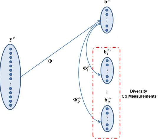
6 Diversified Compressive Sampling 69 6.1 Diversity in Wireless System . . . 706.1.1 System Model . . . 70
6.1.2 Combining Method . . . 71
6.2 Introducing Diversity to CS : Diversified-CS . . . 75
6.2.1 Diversified-CS (dCS) with Disjoint Random Sampling . . . 77
6.2.2 Diversified-CS (dCS) with given CS measurements . . . 78
6.2.3 Noise Reduction of dCS . . . 80
6.3 Comparison with Big-CS . . . 82
6.4 Chapter Review and Next . . . 84
7 Applications to Noise Reduction 87 7.1 CS for Spectrum Sensing . . . 88
7.1.1 Simulation Setup . . . 89
7.1.2 Parameters . . . 90
7.1.3 Numerical Results . . . 93
7.2 CS for 3D Signal Reconstruction . . . 102
7.2.1 Simulation Setup . . . 102
7.2.2 Parameters . . . 105
7.2.3 Numerical Result . . . 105
III
Remedy For Multiplicative Perturbation
113
8 Methods for Reducing Multiplicative Noise 115
8.1 Genie-Aided CS Reconstruction . . . 116
8.2 Suggestion for Practical Method . . . 117
8.2.1 Basis Addition Method . . . 117
8.2.2 Iterative Basis Adjustment Method . . . 119
8.3 Chapter Review and Next . . . 126
9 Application to Wireless Receiver 127 9.1 CS for Wireless Systems . . . 128
9.1.1 A Model of Wireless System . . . 128
9.1.2 Basis Adjustment to Multiplicative Perturbation . . . 132
9.2 Numerical Results . . . 134
9.2.1 Simulation Setup . . . 134
9.2.2 Results . . . 137
9.3 Chapter Review . . . 142
10 Conclusion and Future Work 145 10.1 Diversified-CS for Additive Noise Reduction . . . 146
10.2 Basis Refinement for Multiplicative Noise Reduction . . . 147
10.3 Future Work . . . 147
A Noise Folding of CS 149 A.1 Simple Additive Perturbation in Measurement . . . 149
A.2 Signal Perturbation . . . 150
B Estimating Multiplicative Perturbation 153 B.1 Regression Method with Training Signal . . . 153
CONTENTS xv
C Nonlinear Optimization 157
C.1 Equality Constrained Minimization . . . 158 C.2 Inequality Constrained Minimization . . . 158 C.3 ℓ1 minimization . . . 160
Abbreviation
ADC Analaog-to-Digital Convetrer
BP Basis Pursuit
CoSaMP Compressive Sampling Matching Pursuit
CS Compressive Sampling / Compressed Sensing
bCS Big-CS
dCS Diversified-CS
EGC Equal Gain Combining
IF Intermediate Frequency
LS Least Squares
MP Matching Pursuit
MRC Maximum Ratio Combining
OMP Orthogonal Matching Pursuit
RF Radio Frequency
RIP Restricted Isometry Property
RIC Restricted Isometry Constant
SC Selection Combining
Chapter 1
Introduction
1.1
Background of Compressive Sampling
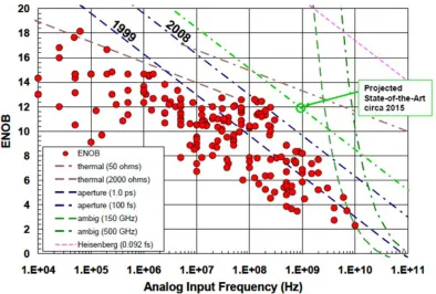
In general, to acquire a continuous signal with analog to digital converter (ADC) the sampling rate of ADC should at least meet the Nyquist rate–twice the max-imum signal frequency. Despite recent advances in semiconductor technology, it is still not easy to meet the Nyquist rate when dealing with very high-frequency signals. Fig. 1.1 shows the allowable frequency of the input signal versus the effec-tive number of bits (ENOB) of ADC [1, 2]. It shows the highest input frequency with 13 ENOB is about 100 MHz at the state of the art in the year of 2008. (At the year of 2012, the speed of a commercial product of ADC is about 160 Mega Samples Per Second (MSPS) [3]. This means that the highest frequency of the baseband signal cannot be bigger than 80 MHz with this ADC.) Then, how can we analyze the whole RF spectrum which is shown in Fig. 1.2? Since it is impossible to analyze the wide-band signal simultaneously with the current ADC, techniques of dividing the wide-band spectrum into multiple bins of small bandwidth and frequency down-conversion are widely used, even though it is much more complex and expensive. If direct sampling is available without any additional processes, this will be a breakthrough in signal processing.
Several techniques have been devised over the past few decades to overcome the requirement of the high sampling rate on the ADC. The most recent one is compressive sampling (CS) [4–10]. CS theory states that the signal can be recon-structed with very few samples if the signal is composed with orthogonal basis functions and the coefficients are sparse. Fortunately, many signals of interest can be represented only with few basis functions.
1.1. BACKGROUND OF COMPRESSIVE SAMPLING 3
Figure 1.1: Effective number of bits (ENOB) of ADC versus input signal fre-quency. [2]
unwanted replicas of spectrum. But this method may be still expensive in case of a sparse signal which does not occupy a continuous range of frequencies in the frequency domain. Further, random (or non-uniform) sampling [12–22] has been introduced. If the signal is sampled randomly, it is known that the aliasing of the signal can be avoided even at the sub-Nyquist rate. However, this method is known to suffer from high noise [14–16].
1.2. CS APPLICATIONS 5
the measurement vector yis noisy, finding the vector xaccurately is not an easy problem. Unless the condition number ofΨis sufficiently small, the recovery will be contaminated with severe noise. To make the matters worse, if the system equation is under-determined, or the number of equations is smaller than that of unknowns, it is very hard to estimate x.
However, under the assumption that x is K-sparse, i.e., only K entries of x are non-zero, we may find x with the sparse approximation technique [27]. CS is an emerging technique of the sparse approximation method. We can recover x even if the number of measurements is much smaller than that of bases. In general, CS can be performed by multiplying the sensing matrix Φ ∈ RM×L to
Ψx=y to reduce the data, where M ≪N ≤L. Then, simply we haveAx =b, whereA=ΦΨ∈RM×N is the measurement matrix and b=Φy∈RM is the CS
measurement vector. Since the number of measurements are reduced from L to
M, the orthogonality of each column of the basis matrix is reduced due to the lack of the measurements. Cand`es and Tao [8] explained the possibility of recovery in the under-determined condition with the concept of the restricted isometry property (RIP). There are various algorithms to find x such as basis pursuit (BP) method [28], convex ℓ1-minimization method [29], non-convex optimization
method [30–32], greedy method [33–35], re-weighted iterative ℓ1-minimization
method [36, 37], NP-hard combinatorial method, etc.
1.2
CS Applications
For an intuitive understanding of the potentials of CS, a simple example of signal reconstruction with CS is demonstrated.
as
f(θ, φ) =
Lf
∑
ℓ=0
ℓ
∑
m=−ℓ
fℓmYℓm(θ, φ), (1.1)
whereLf is the maximum order of SH,Yℓm(θ, φ) is the Laplace spherical harmonic
basis defined as
Yℓm(θ, φ) =
√
(2ℓ+ 1) 4π
(ℓ−m)! (ℓ+m)!P
m
ℓ (cosθ)e jmφ
, (1.2)
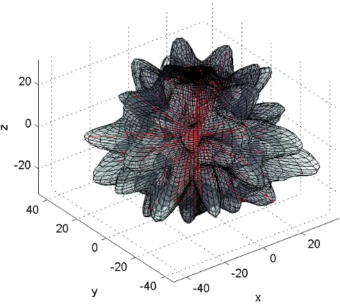
Pℓm is the associated Legendre function, and fℓm are the coefficients of the bases which are sparse. Fig. 1.3(a) shows the reconstruction example of 3D SH signal with CS. For simple demonstration, the sparsity of the coefficients is assumed as
K = 10 out of N = 1326 bases. Its reconstruction of the basis coefficients is shown in Fig. 1.3(b). Only M = 100 measurements are used in estimating 1326 coefficients.
In this example, the important fact about CS can be inferred: few measure-ments may be sufficient for the signal reconstruction as long as the signal is expressed with few basis functions, regardless of the complexity of the signal. The sparsity is the important feature of the signal whether CS can be applied or not in signal reconstruction. Fortunately, many signals of interest can be ex-pressed or approximated with basis functions, and its coefficients are sparse. The potentials of CS are shown in many applications such as
• image signal processing [40–45],
• analog-to-information conversion [46–53],
• wireless communication [54–58],
• spectrum sensing [59–62],
• RADAR [63–67],
1.2. CS APPLICATIONS 7
(a) 3D signal reconstruction via CS. Only 100 measurements are used in the
reconstruction.
0 200 400 600 800 1000
−2 −1.5 −1 −0.5 0 0.5 1 1.5 2
Index of Bases
Coefficient Value
Real Coefficient
CS Reconstructed Coefficient
(b) Reconstructed weights of spherical harmonic bases. 1326 coefficients are
[image:25.612.189.434.124.343.2]estimated with 100 measurements.
1.3
Motivation
While much literature focus on the positive potentials of CS, there are some neg-ative perspectives in CS: perturbation effects of CS. Signal reconstruction with CS is very sensitive to different types of perturbations which can be broadly clas-sified into additive and multiplicative. The additive perturbation, which includes measurement noise [7] and signal noise [68–70], inevitably incurs recovery noise. Signal power should be sufficiently large compared to the amount of additive perturbation [71], and noise folding effect of CS has to be well controlled [68] to apply CS in the presence of additive perturbations (which are independent of the signal). Simply increasing the signal power, however, may incur additional inter-ference noise if there are multiple signal sources. Furthermore, another serious problems may arise when there exist multiplicative perturbations in measure-ments [72, 73]. Multiplicative perturbation may cause a mismatch between the assumed signal basis and that in the measurements, a situation common in prac-tice. Such multiplicative perturbation causes signal-dependent noise and should be minimized for successful application of CS in many engineering systems of interest.
1.3. MOTIVATION 9
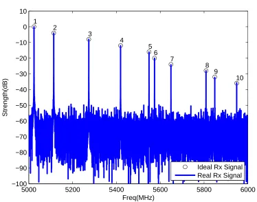
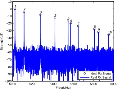
5000 5200 5400 5600 5800 6000 −100 −90 −80 −70 −60 −50 −40 −30 −20 −10 0 10 1 2 3 4 5 6 7 8 9 10 Freq(MHz) Strength(dB)
Ideal Rx Signal Real Rx Signal
(a) Spectrum of the signal which is contaminated
with additive noise.
5000 5200 5400 5600 5800 6000 −100 −90 −80 −70 −60 −50 −40 −30 −20 −10 0 10 1 2 3 4 5 6 7 8 9 10 Freq(MHz) Strength(dB) Dynamic Range
Ideal Rx Signal CS−Recovered Rx Signal
(b) CS-reconstructed spectrum with additive
perturbation.
5000 5200 5400 5600 5800 6000 −100 −90 −80 −70 −60 −50 −40 −30 −20 −10 0 10 1 2 3 4 5 6 7 8 9 10 Freq(MHz) Strength(dB) Dynamic Range
Ideal Rx Signal CS−Recovered Rx Signal
(c) CS-reconstructed spectrum with additive and
[image:27.612.221.411.112.257.2]multiplicative perturbations.
This example shows the perturbation effects of CS when CS is applied to spectrum reconstruction. To use CS more practically, it is highly advisable to reduce the adverse effects from additive and multiplicative perturbations.
1.4
Thesis Overview and Contributions
This thesis makes key observations on the adverse effects of additive and mul-tiplicative perturbations, and illustrates the different impacts of these perturba-tions on the CS signal reconstruction. Most of the thesis is focused on the methods for perturbation reduction. This thesis makes the following contributions:
• We explore the different impacts of additive and multiplicative perturba-tions on CS signal reconstruction.
• For the reduction of the adverse effect of additive perturbation, we propose the diversified-CS (dCS) method which extracts the diversity gain.
• (Application) We apply CS to spectrum sensing for the sampling and the reconstruction of the wide-band signal with a low-speed ADC. Further, the method of dCS is also applied to the spectrum sensing to reduce the spectrum noise. It is shown that the frequency components of the signal buried in the noise due to CS can be found with dCS method. Our technique has a potential to be used in other CS applications where the quality of the recovered signal is an issue.
• For the noise reduction from multiplicative perturbation, we propose an iterative technique of basis adjustment. This technique is practical because no a priori knowledge about which bases are active is required.
1.4. THESIS OVERVIEW AND CONTRIBUTIONS 11
technique is applied to reduce the adverse effect from the multiplicative perturbation. The result shows that this technique removes the noise from multiplicative perturbation successfully.
For clarity, these contributions are organized into three parts.
In Part I, we explore the brief theory of compressive sampling (CS). Before jumping into CS, other fundamental techniques of signal sampling and reconstruc-tion are reviewed in Chapter 2. The basic mathematical concept of CS and its recovery algorithms are shown in Chapter 3. Chapter 4 presents the robust-ness of CS when there exist some perturbations in the measurements. It shows the reconstruction error bounds under the additive and multiplicative perturba-tions, and also compares the error bounds with the least squares (LS) method. Chapter 5 summarizes the noise amplification of CS due to additive and mul-tiplicative perturbations, though CS has the possibility to reduce the recovery noise less than LS in an unstable system compared to LS method.
In Part II, we focus on methods to reduce the noise amplification of CS. Chapter 6 introduces a diversified-CS (dCS) method to reduce the noise from additive perturbation. Diversity technique is widely used in a wireless receiver to improve a signal quality with multi sensors. Diversified-CS (dCS) method, however, which extracts the diversity gain with a single sensor is suggested. To extract diversity gain from a single sensor of CS, we present how to build virtual multiple branches of CS. With virtual multiple branches, multiple recoveries are possible for diversity combining to reduce the noise. Its applications to spectrum sensing and spherical harmonic reconstruction are presented inChapter 7. The simulation results verify that the signal hidden behind the noise can be found much more reliably with dCS method compared to normal CS or LS methods. Even though a toy signal used for simplicity, the dCS method can be applied to other extended applications.
multi-plicative perturbation. This technique is practical because no a priori knowledge about which bases are active is assumed. Instead, the basic idea behind the sug-gested technique is to 1) determine the active bases (initially blindly), 2) adjust the identified active bases to the multiplicative perturbation accordingly, where the adjustment process depends on the application, 3) apply CS recovery to the basis adjusted system of equations, and 4) iterate until desired. Its successful application to a wireless receiver is shown in Chapter 9.
Part I
Exploring CS : Literature Review
Chapter 2
Overview of Signal
Reconstruction
In this chapter, we briefly review the methods of signal sampling and its re-construction. The conventional sampling method such as interpolation method requires Nyquist rate, twice the maximum frequency of the baseband signal. How-ever, we can reconstruct the signal with the least squares (LS) method which does not require sampling at Nyquist rate if the signal consists of a finite number of bases. Furthermore, we can reduce the sampling rate more with compressive sampling (CS) method as long as the signal is sparse in basis domain.
2.1
Methods of Signal Sampling and Its
Recon-struction
2.1.1
Interpolation Method
Let us assume that we want to sample and reconstruct a continuous-time signal
s(t). If we have no information about the signal other than it is band-limited in the range of (0,1/2T) Hz, the signal can be sampled and reconstructed as
s⋆(t) =∑
m
s(tm)φm(t), (2.1)
where s(tm) is the m-th measured sample at an appropriately chosen sampling
time tm and φm(t) is the interpolation function of the m-th sample [74].
Uniform Sampling
If the reconstruction is performed using uniform sampling, i.e., tm = mT, the
interpolation function is the well-known Shannon sampling expansion φm(t) =
sinc(t/T −m) [75], where sinc(t) = sin(πt)/πt.
Non-Uniform Sampling
2.1. METHODS OF SIGNAL SAMPLING AND ITS RECONSTRUCTION17
the signal can be approximated by the Lagrange interpolation function [76–78]
φm(t) =
G(t) (t−tm)G′(tm)
, (2.2)
where
G(t) = (t−t0)
∞
∏
m=1
(1− t
tm
)(1− t
t−m
). (2.3)
For stable reconstruction, the deviation of sampling jitter should be within about 1/4 unit from its corresponding Nyquist instant [77]. It is also proven that any linear combination of irregularly spaced samples whose average rate is above the Nyquist rate is suitable for the reconstruction of the signal [76, 79]. There are also other variations of the interpolation functions [22, 74, 80] to approximate the signal.
Fig. 2.1 shows the reconstructed signal with above two methods. In case of uniform sampling, reconstruction can be done quite easily with the interpolation of the sinc function. More efforts, however, are required for the reconstruction of non-uniform sampling for the calculation of all interpolation functions.
2.1.2
Bandpass Sampling Method
Let us assume that the we have a bandpass signal whose frequency range is (fL, fH) Hz, where fL < fH. This assumption is very natural because many
signals are modulated or converted into bandpass signal for transmission. To sample the signal with the Nyquist rate, there can be two ways in sampling the signal. One is to sample the signal directly at the rate of 2fH. The other is
to sample the signal after frequency down-converting to reduce the maximum frequency of the signal. After frequency down-converting, the frequency range will be (fL−fD, fH−fD), wherefD is down-converting frequency. Then, we can
sample the signal at the rate of 2(fH−fD). In case of the first choice, however, it
(a) Uniform sampling and its reconstruction
(b) Non-uniform sampling and its reconstruction
2.1. METHODS OF SIGNAL SAMPLING AND ITS RECONSTRUCTION19
Figure 2.2: By bandpass sampling, frequency down-conversion and data acquisi-tion are performed simultaneously.
second method is widely and practically used, though it is complex due to the frequency down-conversion.
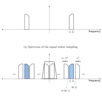
However, it is also possible to sample the signal directly by bandpass sampling if noise folding effect is tolerable [11, 81]. It is also known as under-sampling, harmonic sampling, intermediate frequency (IF) sampling, etc. Frequency down-conversion and data acquisition are done simultaneously by performing bandpass sampling as shown in Fig. 2.2.
Fig. 2.3.(a) and Fig. 2.3.(b) show the spectra of the signal which are before and after bandpass-sampling, respectively. Since the spectrum cannot be overlapped to avoid aliasing, the conditions of
fH ≤nfs−fH,
(n−1)fs−fL≤fL, (2.4)
should be satisfied, where fL and fH are the lowest and highest frequency of the
signal, respectively, fs is the sampling frequency, andn is an integer. Hence, the
acceptable under-sampling rate fs is given by
2fH
n ≤fs ≤
2fL
(a) Spectrum of the signal before sampling.
[image:38.612.100.453.95.429.2](b) Spectrum of the under-sampled signal.
Figure 2.3: Direct frequency down conversion of bandpass sampling.
where
1≤n ≤ ⌊ fH fH −fL⌋
. (2.6)
⌊x⌋ is the largest integer within x. In case that n = 1, the minimum of the allowed rate is the Nyquist rate of the base-band signal. Fig. 2.4 shows the allowed sampling rate of (2.5). The minimum of the allowed sampling rate should be at least 2(fH −fL), two times of the bandwidth. As n gets increased, the allowed
frequency region is getting narrower.
2.1. METHODS OF SIGNAL SAMPLING AND ITS RECONSTRUCTION21
Figure 2.4: The allowable sampling rate for bandpass sampling. White area is the allowed uniform sampling rate versus the band position. [11]
sampling frequency or sampling instant. Furthermore, the signal-to-noise ratio (SNR) is degraded as
SNR = S
Nin+ (n−1)Nout
, (2.7)
where S is in-band signal power, Nin is in-band noise power, and Nout is
out-of-band noise power. This effect is known as noise folding of under-sampling.
2.1.3
Least Squares (LS) Method
This method reconstructs the signal with the assumption that the signal can be approximated with a finite number of known basis functions as
s(t) =Ψ(t)x, (2.8)
where Ψ(t) is the basis set
Ψ(t) =[ψ1(t), ψ2(t), · · · , ψN(t)
]
andx= [x1, x2, ..., xN]T is a coefficient column vector. To approximate the signal,
we have to find the coefficients of bases with given samples [20, 82–84]. We can reconstruct the original signal as
s⋆(t) =Ψ(t)x⋆, (2.10)
where x⋆ is an estimated vector of the basis coefficients. To find x⋆, we use L
samples of yℓ =s(tℓ) forℓ = 1,· · · , L, whereL≥N. Then, we get the following
system of equations
y=Ψx, (2.11)
where y∈CL is the column vector of samples, Ψ∈CL×N is the matrix of bases whose element in row ℓ and column n is Ψℓ,n = ψn(tℓ). The vector x can be
estimated using the least squares (LS) method [24–26] as
x⋆ = arg min
˜
x ∥Ψ˜x−y∥2
=Ψ†y, (2.12)
where ∥ · ∥2 denotesℓ2-norm operation and Ψ† is the pseudo-inverse matrix of Ψ
defined as
Ψ†=
Ψ−1 if L=N
(ΨHΨ)−1ΨH if L > N
,
and ΨH is the Hermitian of Ψ. Sampling time sequence {tℓ, ℓ = 1, ..., L} as
shown in Fig. 2.5 should be selected such that ΨHΨis invertible. In general, we can have a stable recovery if the average sampling rate is sufficiently high above Nyquist rate. However, there have been attempts to have a stable recovery at sub-Nyquist rate [14, 16, 18] with alias-free random sampling method [12].
2.1.4
Compressive Sampling (CS) Method
2.1. METHODS OF SIGNAL SAMPLING AND ITS RECONSTRUCTION23
Figure 2.5: Sampling for LS reconstruction
(CS) [4, 5] under the assumption that x is sparse. Let us assume that we have a matrix Φ ∈ RM×L which reduces the number of samples from L to M. By multiplying the matrix Φ to y = Ψx of (2.11), we get CS measurements. This process is CS observation, and Φ is called CS observation matrix. We obtain measurements which are compressively sampled as
b=Φy=Ax, (2.13)
whereb∈RM is the CS measurements,A=ΦΨ∈RM×N is the CS measurement
matrix, and M ≪ N. Since the number of unknown coefficients, N, is bigger than the number of equations, M, it seems to be impossible to recover the vector x with these measurements.
However, if the vector x is K-sparse, i.e., K = |{j : xj ̸= 0}|, and any 2K
columns ofA are orthogonal, the vector xcan be found as
x⋆ = arg min
˜
x ∥x˜∥1 s.t. b=A˜x, (2.14)
where ∥x˜∥1 :=
∑N
the columns of A, it is possible to find x even in under-determined condition of (2.13). Furthermore, we can also reduce the sampling rate of the elements of the vector y due to the relaxation of the orthogonality of the CS measurement matrix A.
2.2
Nyquist and Compressive Sampling
For comparison of the Nyquist and compressive samplings, here is an intuitive example of signal reconstructions with the both methods.
Example 2.1. We want to reconstruct the signals(t) which consists of sinusoidals as
s(t) =
N
∑
n=1
xnψn(t), (2.15)
where ψn(t) is the n-th sinusoidal basis defined as ψn(t) = cos(2πfnt), and xn is
the coefficient of the n-th basis. For simplicity, the frequency is set to fn = n
Hz. And xn is set to one if n = 3,30,100, and 190, and zero otherwise. To
reconstruct the signal without aliasing, sampling rate should be over the Nyquist rate, i.e., at least 380 Hz in this example. Fig. 2.6(a) shows the reconstruction of the interpolation method with the data samples taken at 440 Hz. On the other hand, Fig. 2.6(b) is the CS signal reconstruction with only 40 data samples that are randomly acquired, about 10 % of the Nyquist rate.
2.2. NYQUIST AND COMPRESSIVE SAMPLING 25
0 0.2 0.4 0.6 0.8 1
−4 −3 −2 −1 0 1 2 3 4
Time(Second)
y
Nyquist Sampling Reconstructed Signal
(a) Nyquist sampling and its reconstruction
0 0.2 0.4 0.6 0.8 1
−4 −3 −2 −1 0 1 2 3 4
Time(Second)
y
Compressive Sampling Reconstructed Signal
(b) Compressive sampling and its reconstruction
2.3
Chapter Review and Next
Chapter 3
Compressive Sampling
In this chapter, we briefly review the theory of compressive sampling (CS) including mathematical basics and CS-recovery algorithms.
3.1
Mathematical Preliminaries and Notations
3.1.1
Vector Spaces
3.1.1.1 Normed Vector
The ℓp-norm of a vector x∈CN is defined for p∈(0,∞) as
∥x∥p :=
(∑N
n=1
|xn|p
)1/p
, (3.1)
and ℓ∞-norm of a vector x is
∥x∥∞:= maxn=1,...,N|xn|. (3.2)
3.1.1.2 Operator Norm of Matrix
The operator norm of a matrix A ∈ CM×N corresponding to the ℓ
p-norm of a
vector x is defined for p∈(0,∞) as
∥A∥p := max∥x∥p̸=0
∥Ax∥p
∥x∥p
, (3.3)
and if p= 2, it is simplified as
∥A∥2 :=σmax(A), (3.4)
where σmax(A) is the largest singular value of A.
In case ofp < 1,∥A∥pis a quasi-norm which satisfies the norm axioms, except
that the triangle inequality is replaced by
∥x+y∥p < C(∥x∥p+∥y∥p), (3.5)
3.1. MATHEMATICAL PRELIMINARIES AND NOTATIONS 29
3.1.1.3 Singular Value and Condition Number of Matrix
A matrix A ∈ CM×N can be decomposed using singular value decomposition
(SVD) into
A=UΣVH, (3.6)
where U ∈ CM×M is a unitary matrix, Σ ∈ CM×N ia a diagonal matrix with
nonnegative real values on the diagonal, and VH ∈ CN×N is another unitary
matrix. The diagonal entries of Σare called singular values denoted with σi, i=
1, ...,min(M, N).
The condition number of A is defined as
κ(A) = σmax(A)
σmin(A)
, (3.7)
where σmax(A) and σmin(A) are maximum and minimum of singular values of
A, respectively.
3.1.2
Sparsity
The ℓ0-norm of a vector xis defined as
∥x∥0 :=|supp(x)|, (3.8)
where supp(x) is the support of xdefined as supp(x) ={n :xn̸= 0}. Although
ℓ0-norm is not a quasi-norm, it is generally called ℓ0-norm.
A vector x is said to be K-sparse if ∥x∥0 ≤K, and
ΣK :={x∈CN :∥x∥0 < K} (3.9)
denotes the set of allK-sparse vectors. If the signal can be expressed asy=Ψx whereΨis a basis matrix and x∈ΣK, the signal ycan be called sparse in basis
3.1.3
Spark and Coherence
The spark of the matrix A is the smallest number of columns of A which are linearly dependent. It can be expressed as
spark(A) := minx̸=0∥x∥0 s.t. Ax=0. (3.10)
And the mutual coherence of the matrix Aintroduced in [85] is defined as
µ(A) := maxi̸=j|aHi aj|, (3.11)
where A is the matrix with normalized columns, ∥ai∥2 = 1, and ai is the i-th
column vector of A.
3.2
Compressive Sampling
3.2.1
ℓ
1-minimization
Since CS is already introduced briefly in the Chapter 2.1.4, let us start with measurements which are compressively sampled with the observation matrix Φ from y=Ψx as
b =Φy=Ax, (3.12)
where b ∈ RM is the CS measurement, and A = ΦΨ ∈ RM×N is the CS
mea-surement matrix. We want to find the vector x∈RN with the CS measurement
vector b. If M is bigger than N, we can estimate x with the LS method of Chapter 2. However, what happens if M is much smaller than N? This will cause under-determined condition on the equation of (3.12), and as a result, it is almost impossible to find the exactx because there are infinitely many solutions to satisfy (3.12). But, if the vectorxisK-sparse, we can findxeven under highly under-determined condition.
Simply, we can find x by searching every combination of K-sparse vector x satisfying b=Ax. This problem can be written as
x⋆ = arg min
˜
3.2. COMPRESSIVE SAMPLING 31
To have the unique solution of x⋆ =x, there is a requirement on the sparsity of
the vector x [86] that
K < spark(A)
2 . (3.14)
However, the problem of solving (3.13) is NP-hard and practically impossible since we need to search every combination of K-sparse vector x. To reduce the complexity of solving (3.13), ℓ0-minimization can be replaced with the ℓ1
-minimization of convex optimization [85] if the sparsity ofx satisfies
K < 1 + 1/µ(A)
2 . (3.15)
Then, the problem of (3.13) can be re-expressed as
x⋆ = arg min
˜
x ∥x˜∥1 s.t. b=A˜x. (3.16)
We can solve this problem easily with a linear program in case of real valued variables and matrices or a second order cone program (SOCP) in the complex-valued setting [29, 87, 88].
It is notable that there was already a practical usage of ℓ1-minimization in
geological sparse signal processing [89–93]. The mathematical background of sparse signal reconstruction, however, is enriched with the topic of CS.
3.2.2
Minimum Required Number of CS Measurements
Since the coherence of the matrix A and the allowable sparsity K of the vector xare totally dependent on the number of CS measurements, there is a minimum required number of CS measurements [94] as
M ≥c·K·logN, (3.17)
10 15 20 25 30 35 40 45 50 0
0.2 0.4 0.6 0.8 1
Number of Measurements
Correlation
0.986(SNR=30dB)
0.954(SNR=20dB)
0.872(SNR=10dB)
1.00 Hz Resolution (N= 200) 0.50 Hz Resolution (N= 400) 0.25 Hz Resolution (N= 800) 0.10 Hz Resolution (N=1000) 0.05 Hz Resolution (N=2000)
Figure 3.1: Correlation between the input and the reconstructed signal versus the number of CS measurements with various sets of bases.
• if the vector x is getting more sparse (smaller K) under the fixed number of bases N,
• if the number of bases N is getting smaller under fixed sparsity K.
3.2. COMPRESSIVE SAMPLING 33
0.4 0.6 0.8 1 1.2 1.4 1.6
0 0.5 1 1.5 2 2.5 3 3.5 4 4.5 5
||Ax2K||22 / ||x2K||22
Probability(%)
δ2K δ2K
Figure 3.2: Restricted Isometry Property
3.2.3
The Restricted Isometry Property
However, the two requirements of (3.14) and (3.15) in finding the exact solution of (3.13) through solving (3.16) are known to be too strict in the sense that the accurate solution can be found with much weaker requirements. In the CS literature [4–8, 95], it is shown that the stable and exact solution can be found with high probability only if any 2K columns ofAare nearly orthogonal. Cand`es and Tao explained the possibility of recovery with the more general concept of the restricted isometry property (RIP). In particular, if in
(1−δ2K)≤ ∥
Ax2K∥22
∥x2K∥22
≤(1 +δ2K), (3.18)
δ2K, termed as the restricted isometry constant (RIC), is quite smaller than one
prob-ability even when M is much smaller than N. Fig. 3.2 shows the RIP and the RIC with the histogram of values of ∥Ax2K∥22
∥x2K∥22 . The implication of the RIP is that
ℓ0-minimization problem of (3.13) has a uniqueK-sparse solution ifδ2K <1 [96].
In addition, if δ2K <
√
2−1, the solution of the ℓ1-minimization problem (3.16)
is same as that of the ℓ0-minimization problem (3.13).
3.3
Signal Recovery Algorithms for CS
There are various algorithms for the sparse signal recovery [27]. These can be roughly categorized as
• Convex ℓ1-minimization method
• Greedy method
• Nonconvex optimization method
• Combinatorial method
• Other : Re-weighting method for noise reduction
3.3.1
Convex
ℓ
1-minimization Method
Since CS recovery with ℓ1-minimization is already described in Chapter 3.2.1,
the brief history of sparse approximation with ℓ1-minimization is explained in
this section. Tibshirani [97] introduced a shrinkage and selection method called LASSO for linear regression. It can estimate the sparse vector x by minimizing the sum of squared errors with the constraint of the sparsity K as
x⋆ = arg min
˜
x
1
2∥A˜x−b∥
2
2 s.t. ∥x˜∥1 ≤K. (3.19)
Basis pursuit denoising (BPDN) method was also introduced [28] as
x⋆ = arg min
˜
x
1
2∥A˜x−b∥
2
3.3. SIGNAL RECOVERY ALGORITHMS FOR CS 35
where λ is a regularization parameter which can sweep out the optimal trade-off curve between the sum of squared errors and the sparsity. If we increase λ, we will have more sparse recovery. The majority of the literature are considering unconstrained optimization methods [98–103]. For some choices of the parameter
λ, the result of this optimization is known to be the same as that of the problem given by
x⋆ = arg min
˜
x ∥x˜∥1 s.t. ∥A˜x−b∥2 ≤ε, (3.21)
whereεis the error bound. The value ofλ, however, which makes these problems equivalent is unknown a priori. Though several approaches for choosing λ are discussed in [104–106], (3.21) seems more convenient and natural because we can adjust the parameter ε according to the amount of the perturbation. Fig. 3.3 illustrates how the solution of (3.21) is found within the error of ε.
3.3.2
Greedy Method
Instead of convex ℓ1-minimization method, greedy method [33–35, 107–123]
re-fines a sparse solution with iterations until some criteria are satisfied. Since it assumes and identifies the support of the signal iteratively, the error can be prop-agated with iterations. It is natural that its accuracy may be worse than that of convex optimization which requires more calculation power. In this section, we briefly review the greedy methods most widely used.
3.3.2.1 Matching Pursuit
Matching pursuit (MP) [33], shown in Algorithm.1, is the most basic greedy method. Basically, it identifies one of the bases which is maximally correlated with the signal, and calculates the coefficient of basis. Hard(xproxy,1) is the
function for producing a vector which has the value of the correlation coefficient at the position of the maximum of |xproxy|. By removing the component of the
Figure 3.3: Geometrical illustration of the convex ℓ1-minimization and
non-convex ℓq(0< q <1)-minimization reconstruction with error ε.
further iterations, we can find active bases of the signal. A variant method of MP in choosing bases is shown in [108].
3.3.2.2 Orthogonal Matching Pursuit
3.3. SIGNAL RECOVERY ALGORITHMS FOR CS 37
Algorithm 1 MP
Input : Matrix A, measurement vector b Output : x⋆
(Start) x⋆ =0,r =b repeat
xproxy =AHr
z = Hard(xproxy,1)
x⋆ =x⋆+z r =b−Az
until {stopping criterion true}
Algorithm 2 OMP
Input : Matrix A, measurement vector b Output : x⋆
(Start) x⋆ =0,r =b
repeat
xproxy =AHr
z = Hard(xproxy,1)
T = supp(z)∪supp(x⋆)
x⋆|T =A†Tb, x ⋆|
Tc =0 r =b−Ax⋆
3.3.2.3 CoSaMp
Compressive sampling matching pursuit (CoSaMP) [35] is almost the same as OMP except it uses the characteristics of 2K-RIP of (3.18). It finds 2K bases which have maximum correlations with the signal and calculates the coefficients of 2K bases. Then, it chooses K bases after recalculating the coefficients of the identified bases with LS method and removes the components of the chosen K
bases from the signal. With iterations, more accurate coefficients can be found as shown in Algorithm.3. This method, however, requires a priori knowledge about the sparsity K.
Algorithm 3 CoSaMP
Input : Matrix A, measurement vector b, sparsity level K
Output : K-sparsex⋆
(Start) x⋆ =0,r =b
repeat
xproxy =AHr
z= Hard(xproxy,2K)
T = supp(z)∪supp(x⋆)
v|T =A†Tb, v|Tc =0 x⋆ = Hard(v, K)
r =b−Ax⋆
until {stopping criterion true}
3.3.3
Non-convex
ℓ
q-minimization Method
It is known that ℓq(0 < q < 1)-minimization can replace ℓ1-minimization in
solving sparse signal with fewer measurements [30–32, 124]. Fig. 3.3 compares
3.4. CHAPTER REVIEW AND NEXT 39
Figure 3.4: Reshapingℓ1-ball to avoid a wrong intersection point. [36]
3.3.4
Re-weighting
ℓ
1-minimization Method
In solving the ℓ1-minimization problem, the intersection point of the ℓ1-ball and
the constraint is selected as the solution of the problem as shown in Fig. 3.4(a). However, if there is noise in the signal, there is high probability to have a wrong intersection point as a solution as shown in Fig. 3.4(b). In this case to avoid the wrong intersection point, we can reshape theℓ1-ball thinly as conceptually shown
in Fig. 3.4(c). This method is introduced in [36, 37] and it can be performed by re-weighting the coefficients of bases. Algorithm.4 outlines the steps.
3.4
Chapter Review and Next
Algorithm 4 Reweightedℓ1 minimization
Input : Matrix A, measurement vector b, some small constant ϵ
Output : x⋆
(Start) W =I repeat
x⋆ = arg min
˜
x∥Wx˜∥1 s.t. b=A˜x. Wnn = 1/(x⋆(n) +ϵ) for n= 1, .., N
until {stopping criterion true}
Chapter 4
Robustness of CS to
Perturbations
In this chapter, CS robustness against additive and multiplicative pertur-bations will be investigated. These perturpertur-bations have adverse effects on CS recovery and can cause serious noise on CS-recovered signal.
4.1
CS Recovery With Perturbations
Let us assume that the original signal before CS is distorted with perturbations is given by
yp = (Ψ+ ∆Ψ)(x+ ∆x) + ∆y, (4.1)
where ∆Ψis the mismatch between the assumed and the real basis of the signal, ∆x is the signal perturbation to x, and ∆y is the additive measurement noise.
Suppose hat we want to sample the measurement compressively with CS ob-servation matrix Φ. It is true that there can be also perturbation on the CS observation matrix Φ, but we are not considering the perturbation on CS ob-servation for fair comparison with non-CS recovery. After compressive sampling with the CS observation matrix Φ, we obtain CS measurements of
bp = (A+ ∆A)(x+ ∆x) + ∆b, (4.2)
where ∆A=Φ∆Ψis CS multiplicative perturbation, and ∆b=Φ∆yis additive perturbation added to the CS measurement. Comparing the perturbed measure-ment (4.2) with the noise-free measuremeasure-ment (3.12), the perturbed measuremeasure-ment can be written as
bp =b+nb, (4.3)
where nb is the CS noise from perturbations. nb can be decomposed into three
terms as
nb=nbmul+nbsp + ∆b, (4.4)
4.1. CS RECOVERY WITH PERTURBATIONS 43
Since the measurement b is contaminated with the noise nb, x should be
searched within the noise bound εb as
x⋆ = arg min
˜
x ∥x˜∥1 s.t. ∥A˜x−b
p∥
2 ≤εb, (4.5)
where εb is the upper bound on the total noise nb. Then, the difference between the recovered coefficient vectorx⋆and the exact coefficient vectorxis the recovery
noise measured as
nx =x⋆−x. (4.6)
However, the impacts of the above three perturbations on the recovery noise nx are quite different, and it is worth investigating how these perturbations have effects on the recovery noise.
4.1.1
Additive Perturbation
The CS noise of (4.4) can be classified into two perturbation terms as
nb =nbmul +nbsp + ∆b
| {z }
nbadd
=nbmul +nbadd, (4.7)
where nbmul is a multiplicative noise, and nbadd is an additive noise measured as nbadd =nbsp + ∆b. In this section, the effect of the additive perturbation nbadd to CS measurement will be investigated.
4.1.1.1 Measurement Perturbation
For simplicity, we consider only an additive CS measurement noise ∆b, i.e., ∆A= 0and ∆x=0. This model covers many situations since the additive perturbation to the measurement is very common. The CS measurements are simply written as
The recovery noise will be different according to the type of the additive CS measurement noise ∆b. We will consider two types of the noise, bounded noise and Gaussian noise, as below:
Bounded Noise[7, 96]
With the assumption that the additive CS measurement noise ∆b is bounded by ∥∆b∥2, the recovery noise is known to obey, ifδ2K <
√ 2−1,
∥x⋆−x∥2 ≤C0
∥x−√xK∥1
K +Cadd∥∆b∥2, (4.9)
where
C0 = 2
1−(1−√2)δ2K
1−(1 +√2)δ2K
, (4.10)
and
Cadd =
4√1 +δ2K
1−(1 +√2)δ2K
. (4.11)
If x isK-sparse, the recovery noise will be bounded as
∥x⋆−x∥2 ≤Cadd∥∆b∥2. (4.12)
There is another model of bounded noise, where the maximum element of the noise is bounded as ∥AT∆b∥∞ ≤λ. Under this noise model, we can recover the signal with a different algorithm called the Dantzig selector [125]. If∥AT∆b∥∞ ≤
λ,x can be estimated as
x⋆ = arg min
˜
x ∥x˜∥1 s.t. ∥A
T(A˜x−bp)∥
∞≤λ, (4.13)
as long as δ2K <
√
2−1. The recovery noise ofK-sparse vector is known to obey
∥x⋆−x∥2 ≤CDantzig
√
Kλ, (4.14)
where
CDantzig = 4
√ 2 1−(1 +√2)δ2K
. (4.15)
Gaussian Noise[126]
Since it is very natural to assume the noise as i.i.d Gaussian noise, we will regard the noise before CS ∆y as i.i.d. Gaussian noise with covariances of σ2
4.1. CS RECOVERY WITH PERTURBATIONS 45
Thus, the noise after CS, ∆b = Φ∆y, will be also i.i.d. Gaussian noise whose covariance will be σ2
0I if we have the CS observation matrix of ΦΦ
T = I. The
upper bound of ∥∆b∥2 can be found using Markov inequality. The tail property
of Gaussian noise ∆bshown in [126] presents by using standard properties of the Gaussian distribution that there exists a constant c0 such that
P((1 +ϵ)√M σ0 ≤ ∥∆b∥2 )
≤exp(−c0ϵ2M), (4.16)
where P(E) denotes the probability that the eventE occurs and ϵ is a constant bigger than zero. If we setϵ to one, ∥∆b∥2 will be bounded as
∥∆b∥2 <2σ0
√
M , (4.17)
with probability of 1−exp(−c0M). Then, the CS recovery noise with the influence
of the Gaussian additive noise whose covariance is σ2
0Iwill be bounded as
∥x⋆−x∥2 ≤2σ0
√
M Cadd (4.18)
with probability of 1−exp(−c0M).
We can also consider the recovery noise bound of the Dantzig selector in the context of Gaussian noise. If A is a matrix whose columns have unit norm, the elements ofAT∆bare also Gaussian noise with zero mean and varianceσ02. Using the tail property of the Gaussian distribution, we have
P(|[AT∆b]i|> tσ0
)
≤exp(−t2/2) (4.19)
for i= 1,2, ..., N. We obtain, by using the bound over all i,
P(∥AT∆b∥∞ >2√logN σ0 )
≤Nexp(−2 logN) = 1
N, (4.20)
by settingt= 2√logN. Thus, since we can set λas 2√logN σ0, we have another
noise bound of the Dantzig selector as
∥x⋆−x∥2 ≤2σ0 √
KlogN CDantzig (4.21)
Comparing the two noise bounds of (4.18) and (4.21), we can find that there is quite a difference. With (4.18), even in case thatM andN are fixed, we cannot explain about the recovery noise even if K is reduced , while we can expect the noise reduction with (4.21). However, in general, the noise bound of (4.18) is widely used except that the sparsity K is changing.
4.1.1.2 Signal Perturbation
Signal perturbation can be defined as unwanted and unknown noise ∆x added to the signal x. This phenomenon is very common if there is a co-channel in-terference or if the signal vector x is already contaminated with noise. The CS measurements affected by the signal perturbation will be given by
bp =A(x+ ∆x)
=Ax+nbsp, (4.22)
wherenbsp is the noise due to the signal perturbation given bynbsp =A∆x. nbsp seems to be only additive noise, but the characteristics of nbsp is quite different compared to the direct additive perturbation ∆bon the CS measurement of (4.8). To characterize effects of noise in a statistical way, we assume that ∆xis also i.i.d. Gaussian noises with covariances of σ2
∆I. Then, the covariance of the signal
perturbation noise nbsp will be calculated as
P= Cov(nbsp)
=ACov(∆x)AT, (4.23)
where Cov(·) is the covariance operation. If we assume that the columns of A have unit norm andAAT can be approximated by (N/M)I,nbsp will be modeled as i.i.d. Gaussian noise with covariance
P=σ∆2AAT
4.1. CS RECOVERY WITH PERTURBATIONS 47
where σ2
s =σ∆2N/M [Appendix A]. Furthermore, the approximation is accurate
even when AAT is not proportional to the identity matrix [70]. (4.24) shows that the signal perturbation causes the noise amplification in the CS recovery with the factor of compression ratio of N/M [68–70], which is very similar to the noise folding effect of undersampling [11]. Since the signal perturbation noise nbsp is i.i.d. Gaussian noise, its upper bound can be approximated in the same way of (4.17) as
∥nbsp∥
2 <2σs
√
M (4.25)
with high probability. Then, the CS recovery noise will be bounded by
∥x⋆−x∥2 ≤2σs
√
M Cadd (4.26)
with high probability.
4.1.1.3 Both Measurement and Signal Perturbations
We consider both measurement and signal perturbations in CS measurements. The CS measurements will be given by
bp=A(x+ ∆x) + ∆b
=Ax+A∆x| {z+ ∆b}
nbadd
, (4.27)
where nbadd is the total additive perturbation on CS measurements given by
nbadd =A∆x+ ∆b. (4.28)
If we assume that ∆x and ∆b are both i.i.d. Gaussian as already described in the previous sections, the covariance of nbadd can be approximated by
Q≈σadd2 I, (4.29)
where σadd = √
σ2
0I+σ∆2N/M.
By the tail property of Gaussian variable, the total additive noise nbadd will be bounded as
∥nbadd∥
2 <2σadd
√
M = 2
√ M σ2
with high probability. Hence, the noise bound of CS recovery obeys
∥x⋆−x∥2 ≤Cadd∥nbadd∥2
< Cadd·εadd (4.31)
with high probability.
4.1.2
Multiplicative Perturbation
More detrimental type of perturbation is multiplicative perturbation in the mea-surement [72, 127]. The meamea-surement under this perturbation model will be expressed as
bp = (A+ ∆A)x
=Ax+nbmul, (4.32)
where nbmul = ∆Ax. Since ∆A causes basis mismatch in the measurements, signal-dependent noise nbmul is incurred due to multiplicative perturbation.
By the quantitative modeling method, multiplicative perturbation is modeled as
∥∆A∥(2K) ∥A∥(2K) ≤ε
(K)
A , (4.33)
whereε(AK)is relative upper bound on multiplicative perturbation. ∥ · ∥(2K)denotes the maximum spectral norm of all K-column sub-matrices of a matrix which consist of any K columns of the matrix. It is shown in [72] that, if 2K-RIC satisfies
δ2K <
√ 2
(
1 +ε(2AK))2
−1, (4.34)
the reconstruction error of the K-sparse vector xobeys
∥nx∥2 ≤Cmul∥nbmul∥2, (4.35)
where Cmul is a constant given by
Cmul =
4√1 +δ2K(1 +ε(2AK))
1−(1 +√2)((1 +δ2K)(1 +ε
(2K)
A )2−1
4.1. CS RECOVERY WITH PERTURBATIONS 49
Since the ℓ2-norm of the multiplicative noise nbmul is bounded as
∥nbmul∥
2 ≤ ∥
∆Ax∥2
∥Ax∥2
∥b∥2
< ∥∆A∥ (K) 2 ∥x∥2
√
1−δK∥x∥2
∥b∥2
≤ √
1 +δK
√ 1−δK
ε(AK)∥b∥2 =εmul, (4.37)
with the assumption that b̸= 0, the CS recovery noise under the multiplicative perturbation will be bounded as
∥x⋆−x∥2 < Cmul·εmul. (4.38)
4.1.3
General Perturbation
A more general case which includes additive, multiplicative and signal perturba-tions, the CS measurements is given by
bp = (A+ ∆A)(x+ ∆x) + ∆b
= (A+ ∆A)x+ (A+ ∆A)∆x+ ∆b
| {z }
nbadd
=Ax+nbmul+nbadd, (4.39)
where nbmul = ∆Ax and nbadd = (A+ ∆A)∆x+ ∆b. If ∆A∆x is negligible compared to the total amount of additive noisenbadd,nbadd can be approximated by
nbadd ≈A∆x+ ∆b, (4.40)
which is almost the same as (4.28). Then, the covariance ofnbadd is approximated by
Q≈σadd2 I= (σ02+σ2∆N
M)I. (4.41)
This is known to be also true as long as ∆Adoes not break the low coherence or the low RIP of A+ ∆A[70]. Hence, the total noise nb is bounded as
∥nb∥2 ≤ ∥nbmul∥2+∥nbadd∥2
![Figure 1.2: United States Frequency Allocation Chart. [23]](https://thumb-us.123doks.com/thumbv2/123dok_us/8116052.238232/22.612.136.427.100.710/figure-united-states-frequency-allocation-chart.webp)
![Figure 3.4: Reshaping ℓ1-ball to avoid a wrong intersection point. [36]](https://thumb-us.123doks.com/thumbv2/123dok_us/8116052.238232/57.612.129.493.114.345/figure-reshaping-ball-avoid-wrong-intersection-point.webp)